“Fuzzy Band Gaps”: A Physically Motivated Indicator of Bloch Wave Evanescence in Phononic Systems

Abstract

Phononic crystals (PCs) have been widely reported to exhibit band gaps, which for non-dissipative systems are well defined from the dispersion relation as a frequency range in which no propagating (i.e., non-decaying) wave modes exist. However, the notion of a band gap is less clear in dissipative systems, as all wave modes exhibit attenuation. Various measures have been proposed to quantify the “evanescence” of frequency ranges and/or wave propagation directions, but these measures are not based on measurable physical quantities. Furthermore, in finite systems created by truncating a PC, wave propagation is strongly attenuated but not completely forbidden, and a quantitative measure that predicts wave transmission in a finite PC from the infinite dispersion relation is elusive. In this paper, we propose an “evanescence indicator” for PCs with 1D periodicity that relates the decay component of the Bloch wavevector to the transmitted wave amplitude through a finite PC. When plotted over a frequency range of interest, this indicator reveals frequency regions of strongly attenuated wave propagation, which are dubbed “fuzzy band gaps” due to the smooth (rather than abrupt) transition between evanescent and propagating wave characteristics. The indicator is capable of identifying polarized fuzzy band gaps, including fuzzy band gaps which exists with respect to “hybrid” polarizations which consist of multiple simultaneous polarizations. We validate the indicator using simulations and experiments of wave transmission through highly viscoelastic and finite phononic crystals.

1. Introduction

In nearly 30 years since the development of the first phononic crystal (PC) [1], a plethora of interesting properties of PCs has been discovered, foremost of which are band gaps, frequency ranges over which elastic wave propagation is forbidden. Band gaps give PCs a diverse range of applications including vibration suppression [2], waveguiding [3], and energy harvesting [4]. Band gaps are easily defined and identified for undamped PCs, which constitute the majority of published works, but are much more difficult to define and identify in damped PCs. As all real materials exhibit damping, understanding band gaps in damped PCs is thus critical to developing real-world applications for PCs. The purpose of this work is to develop a method for defining and identifying band gaps in damped PCs which is based on measurable physical quantities. Such a method is amenable to experimental verification, which allows the performance of physically realized PCs to be assessed relative to model predictions.

Damping in PCs, and the related structures known as acoustic metamaterials, has been an increased focus of research in the last decade. Damping creates phenomena not found in undamped PCs, such as “wavenumber band gaps” [5], and conversely, PCs can create novel damping behaviors not found in the bulk material, such as anisotropic dissipation [6]. Damping is also unintentionally but inevitably present in many PCs which rely on key properties of materials that also happen to be damped. For example, locally resonant PCs [7], pattern transformation-tunable band gaps [8], and magnetically-tunable band gaps [9,10,11] were enabled by the low stiffness, ability to undergo large strains, and magnetic tunability of elastomers, respectively. The inclusion of damping strongly affects the PC band structure, causing pronounced smoothing of dispersion curves [12] or a re-ordering of dispersion curves known as “branch overtaking” [13,14]. In damped band structures, either frequency [13], wavenumber [12], or both [15] become complex-valued, which creates challenges for identifying band gaps. In some works, such as those previously cited on elastomeric PCs [7,8,9,10,11], damping is neglected to simplify the interpretation of the band structures. However, a full understanding of wave propagation can only be obtained when damping is considered, due to the strong effect of damping on the band structure. In particular, the need to understand the damped band structure of the magneto-active metastructures studied in [11] provided a strong initial impetus for the current work, as the elastomeric material from which they were fabricated is highly viscoelastic.

In works where damping is included, various methods have been developed to aid in interpreting band structures, which generally depend upon the class of waves that are studied: free waves or driven waves. Free waves can decay in time and in space [15]. However, the most common analysis technique for free wave solutions is the “indirect” or $\omega \left(k\right)$ method, which proceeds by prescribing a real-valued Bloch wavenumber and solving the resulting eigenvalue problem for the complex frequency [14,16], yielding waves which decay in time but not in space. The damping ratio $\zeta$ has become a standard figure of merit to characterize the temporal decay of the wave and has been used, e.g., to study the phenomenon known as metadamping [17,18,19] and to study the transition between viscously and viscoelasticly damped PCs [20]. An alternative figure of merit that has found limited use is the quality factor [21]. On the other hand, driven waves decay in space but not in time and are obtained using the “direct” or $k\left(\omega \right)$ method, by prescribing real frequencies and computing complex wavenumbers. Band structures for damped driven waves are much more difficult to interpret than band structures for undamped driven waves, because all wave modes are propagative (with spatial decay), and the cusps of the dispersion curves become highly rounded, even for weak damping [12]. The rounding of the dispersion curves makes it difficult to identify band gap edge frequencies and has led several authors to use various figures of merit to quantify the wave decay: the minimum imaginary component of all wavenumbers at a given frequency [22,23], the minimum imaginary component normalized by wavenumber absolute value [24], and the effective loss factor [22,25]. In [22,24], the respective figures of merit are visualized with a light-to-dark shading scheme to visually indicate regions of highly attenuated wave propagation. However, the lack of a standardized figure of merit illustrates the ongoing difficulties of identifying band gaps for damped driven wave propagation.

An additional difficulty lies in identifying polarized band gaps, which may also exist in PCs even when complete band gaps cannot be found. Polarized band gaps have long been studied in 2D PCs, where different band gaps are observed for modes with in-plane displacements and out-of-plane displacements, see, e.g., in [26]. More recently, polarized band gaps with other polarizations (flexural, torsional, longitudinal) were discovered in lattice-based PCs [11,27,28,29]. Identification of polarized band gaps is more complicated than complete band gaps, because it requires a method to classify the polarization of each Bloch mode shape. In [11,27,28,29], manual inspection of the Bloch mode shapes was used to determine the subset of modes that align with the polarization of interest, which is problematic as it requires judgment calls of whether each mode is significant for a given direction. Additionally, the PCs in [11,27,28,29] were physically realized using polymeric and elastomeric materials which have significant damping. Including damping in the band structure computation necessitates simultaneous consideration of the polarization and rate of decay for each mode, and to the authors’ knowledge, no such method has yet been proposed.

Band gaps may also be studied by considering finite structures created by truncating infinite PCs. The distribution of the finite structure’s natural frequencies is dictated by the dispersion relation of the unit cell [30,31], which prevents natural frequencies from falling within the band gap, causing a deep trough in vibration transmission in the band gap frequencies. The transmission trough increases in depth with the number of unit cells in the truncated structure [32], which is due to the larger number of poles in the frequency response function that lie below the band gap [33]. It has further been shown that the dissipated power in a finite periodic structure is confined near the source for excitation frequencies within the band gap [34], which has been proposed as an alternate means to identify band gaps from finite structures. The correspondence between the dynamics of infinite and finite PCs is especially significant as it allows for experimental verification of band gap existence. However, the existence of damping in all real materials causes smoothing of the transmission trough edges (see, e.g., in [25]), which makes experimental identification of band gaps difficult for highly damped materials [11].

The goal of this work is to develop a method by which polarized band gap-like frequency ranges can be systematically identified in damped PCs. As damped PCs may exhibit strong wave attenuation due to Bragg scattering, yet possess no true band gaps due to the effect of dissipation on the eigenmodes, we introduce the term “fuzzy band gaps” for frequency ranges with strong spatial attenuation of waves which may or may not be true band gaps. We define a fuzzy band gap as any frequency range where the transmitted wave amplitude through a finite periodic structure is less than a prescribed threshold. Though the threshold wave amplitude is arbitrary, it can be chosen based on physical grounds or engineering requirements, such as the maximum allowable vibration amplitude of a structure. Although “fuzziness” in PCs can arise from multiple sources, such as disorder or parasitic resonators, in this article we focus only on fuzziness arising from dissipation. We then select a measurable physical quantity (e.g., displacement or force) as a measure of wave amplitude, approximate the transmitted wave amplitude in a finite PC using a weighted superposition of the Bloch waves, and search for fuzzy band gaps by comparing the transmitted wave amplitude to the threshold amplitude. The use of a measurable physical quantity allows the fuzzy band gaps thus obtained to be directly verified by experiments. We first validate the evanescence indicator for a simple 1D viscoelastic diatomic lattice and show that the predicted fuzzy band gaps agree well with simulations of the vibration transmission through finite PCs. The “fuzzy” moniker arises from the fact that the evanescence indicator reveals smooth transitions between propagating and decaying wave behavior, which make the edges of a fuzzy band gap appear like an out-of-focus or “fuzzy” photo. We next validate the evanescence indicator on “magneto-active metastructures”, which are damped PCs with complex 3D geometry based on prior work [11], using a combination of finite element method simulations and experiments. We show that the evanescence indicator is capable of identifying fuzzy band gaps with respect to arbitrary wave polarizations, including hybrid polarizations that consist of a superposition of two or more simple polarizations. Because of its applicability to damped PCs with complex geometries and its direct link to experimental results, the evanescence indicator is a powerful tool for interpreting damped band structures of PCs fabricated from real materials.

2. Theory

In this section, we derive an “evanescence indicator”, a figure of merit which quantifies how strongly waves are attenuated in a periodic structure at a given frequency. To compute this evanescence indicator only requires knowledge of the dispersion relation $k\left(\omega \right)$ for an infinite periodic structure, the accompanying Bloch wave mode shapes, a threshold displacement amplitude of interest $u_{thres}$, and the number of unit cells N that defines the extents of a finite periodic structure of reference. This method is applicable for both undamped and damped structures with 1D periodicity.

2.1. Background

According to the Bloch theorem, as adapted to elastodynamics, waves propagating in periodic structures can be described by a basis of eigenfunctions having the form

$$\begin{array}{c}\hfill \mathit{u}(\mathit{x},t)=e^{i(\mathit{k}·\mathit{x}-\lambda t)}\widehat{\mathit{u}}\left(\mathit{x}\right),\end{array}$$

(1)

where $\mathit{x}$ and t are the spatial and time coordinates, respectively; $\mathit{u}$ is the displacement field; $\widehat{\mathit{u}}$ is a function with the same periodicity as the periodic structure; $\mathit{k}$ is the Bloch wavevector; and $\lambda$ is the angular frequency. Quantities in boldface denote vectors and $\mathit{u}$, $\widehat{\mathit{u}}$, $\mathit{k}$, $\lambda$ may all be complex-valued, depending on the frequency of excitation and the material properties of the structure.

For driven wave propagation, i.e., waves which are excited by a harmonic displacement or force and decay in space but not in time, the “direct” or $k\left(\omega \right)$ method is used to solve the dispersion relation. This method proceeds by prescribing a real-valued angular frequency $\omega$ and solving the resulting eigenvalue problem for the Bloch wavevector $\mathit{k}$. Writing the Bloch wavevector in terms of its real and imaginary parts and substituting $\mathit{k}={\mathit{k}}_R+i{\mathit{k}}_I$ and $\lambda =\omega +0i$ into (1) yields

$$\begin{array}{c}\hfill \mathit{u}(\mathit{x},t)=e^{-{\mathit{k}}_I·\mathit{x}}{e}^{i({\mathit{k}}_R·\mathit{x}-\omega t)}\widehat{\mathit{u}}\left(\mathit{x}\right).\end{array}$$

(2)

It is evident that the imaginary-valued exponential function $e^{i({\mathit{k}}_R·\mathit{x}-\omega t)}$ governs the spatial and temporal oscillation of the wave, while the real-valued exponent $e^{-{\mathit{k}}_I·\mathit{x}}$ defines an “envelope” that governs the spatial growth or decay of the wave. If the wavevector is real-valued, i.e., ${\mathit{k}}_I=\mathit{0}$, then the wave undergoes no change in amplitude as it propagates and is termed a “propagating” wave. However, for complex-valued $\mathit{k}$, the wave amplitude will decrease with increasing ${\mathit{k}}_I·\mathit{x}$ and the wave is known as an “evanescent” wave. As an evanescent wave propagates through a medium of infinite extent, that is, $\mathit{x}\to \pm \infty$, the wave amplitude decays to zero as ${\mathit{k}}_I·\mathit{x}\to \infty$.

In undamped periodic media, the dispersion relation can be partitioned into discrete “pass bands” (frequency ranges where at least one real-valued $\mathit{k}$ exists) and “stop bands” or “band gaps” (frequency ranges where all $\mathit{k}$ are complex, i.e., all waves are evanescent). Within a band gap, wave transmission in an unbounded medium is prohibited, because all wave modes decay to zero amplitude.

However, it is not so straightforward to define band gaps in finite structures or in damped periodic structures. In finite periodic structures created by truncating an infinite structure, a nonzero transmission is observed at all frequencies, even within the band gap, because $e^{-{\mathit{k}}_I·\mathit{x}}\ne 0$ for any finite ${\mathit{k}}_I$, $\mathit{x}$. In damped periodic structures, all $\mathit{k}$ are complex, so all wave modes are evanescent according to the traditional definition. In each of these cases, the rate of spatial decay of the wave amplitude (which depends on ${\mathit{k}}_I$) becomes important for characterizing the effectiveness of the phononic crystal at suppressing wave transmission. The developed evanescence indicator uses this basic concept of faster/slower wave decay and links it to measurable physical quantities such as displacement or force, so that band gaps in damped phononic crystals can be systematically defined.

2.2. Derivation of Evanescence Indicator

Our general approach to defining an evanescence indicator for damped systems is as follows. First, we select a finite structure of reference for which the wave attenuation is measured and choose a physical quantity (e.g., stress or displacement) as a measure of wave amplitude. For concreteness, we study two examples in which the displacement at a single point and the average displacement magnitude over several points are selected to characterize the wave amplitude. Next, we approximate the wave amplitude for all frequencies of interest using information directly extracted from the dispersion relation: a weighted summation of the Bloch mode shapes, so that the contributions of all wave modes are considered simultaneously. The amplitude is calculated at two locations (“input” and “output”) and the normalized transmission (output divided by input) is computed. Finally, we define “fuzzy band gaps” using a threshold value of normalized transmission as the criterion for fuzzy band gap existence: if the transmission is greater than the threshold transmission, there is no fuzzy band gap, and if the transmission is less than the threshold transmission, a fuzzy band gap is considered to exist. Two methods are discussed for determining the weights in the summation of Bloch modes, because the correct calculation of the weights is critical to accurately identifying the fuzzy band gaps.

Consider a structure which is infinitely periodic in the x-direction and of finite extent in the y- and z-directions. The structure is excited by arbitrary forcing (prescribed forces and/or displacements) at a real frequency $\omega$. Bloch wave propagation occurs in the x-direction only, so that $\mathit{k}·\mathit{x}=kx$, where the scalar k is the magnitude of the wavevector $\mathit{k}$. As the Bloch wave modes form a basis for the displacement field, the total displacement field of the wave can be expressed as a superposition of Bloch waves:

$$\begin{array}{c}\hfill \mathit{u}(\mathit{x},t;\omega )=\sum _j{A}_j{e}^{-k_{j,I}x}{\widehat{\mathit{u}}}_j\left(\mathit{x}\right)e^{i\left(k_{j,R}x-\omega t\right)},\end{array}$$

(3)

where $A_j$ is the amplitude of the jth Bloch wave having wavenumber $k_j=k_{j,R}+i{k}_{j,I}$ and mode shape ${\widehat{\mathit{u}}}_j$, and the summation is carried out over all Bloch modes existing at frequency $\omega$. As all Bloch wave modes occur in pairs ($+\mathit{k}$, $-\mathit{k}$) and the summation is over all Bloch wave modes, waves propagating in both the $+x$ and $-x$ directions are present in the summation, and the modal amplitudes $A_j$ are chosen to give a physically realistic solution (i.e., with $A_j=0$ for physically unrealistic wave modes). We define the “input displacement” as the displacement $\mathit{u}({\mathit{x}}_i,t)$ of the structure at the point ${\mathit{x}}_i={[x_i,y_i,z_i]}^T$ and the “output displacement” as the displacement $\mathit{u}({\mathit{x}}_o,t)$ of the structure at the point ${\mathit{x}}_o={[x_o,y_o,z_o]}^T$. Note that the terms “input” and “output” are chosen merely to reflect the convention that transmission is output divided by input; the locations of ${\mathit{x}}_i$ and ${\mathit{x}}_o$ are arbitrary and are left to the user to be chosen as appropriate for a given application. As the dynamics of finite periodic structures are known to resemble the dynamics of the corresponding infinite structure [32], we propose that the displacement at points ${\mathit{x}}_n,n\in i,o$ in a finite periodic structure can be approximately expressed by Equation (3). This approximation is made in order to link the information contained in the dispersion relation to the finite structure upon which the fuzzy band gap definition is based. The magnitudes of the displacements at the points ${\mathit{x}}_n$ are

$$\begin{array}{c}\hfill \left|\mathit{u}({\mathit{x}}_{\mathit{n}};\omega )\right|=\left|\sum _j{A}_j{e}^{-k_{j,I}{x}_n}{\widehat{\mathit{u}}}_j\left({\mathit{x}}_n\right)e^{i{k}_{j,R}{x}_n}\right|,\end{array}$$

(4)

which forms the basis for our proposed evanescence indicator. Here, n is independently taken as $i,o$ to indicate that the displacement magnitude is evaluated at the points ${\mathit{x}}_i$ and ${\mathit{x}}_o$.

To develop the definition of a fuzzy band gap, we first give an alternate definition of a band gap. In infinite undamped periodic structures, band gaps are identified by seeking frequencies ${\omega }_{BG}$ where all Bloch wavenumbers $k_j$ are complex or imaginary. Placing the input point ${\mathit{x}}_i$ at the origin and the point ${\mathit{x}}_o={[\infty ,0,0]}^T$ an infinite distance away on the x-axis, it is clear that the the transmitted wave amplitude $\left|u\right|$ is 0 within the band gap, as

$$\begin{array}{c}\hfill \underset{x_o\to \infty }{lim}{e}^{-k_{j,I}{x}_o}=0\forall k_{j,I}>0,\end{array}$$

(5)

and all wavenumbers have nonzero $k_{j,I}$ within the band gap. Therefore, a band gap can be equivalently defined as a range of frequencies ${\omega }_{BG}$ for which the displacement amplitude transmitted through an infinite structure is equal to a threshold amplitude, namely 0,

$$\begin{array}{c}\hfill \left\{{\omega }_{BG}\in \mathbb{R}\left|\underset{x_o\to \infty }{lim}\left|u(x_o,t;{\omega }_{BG})\right|=0\right.\right\}.\end{array}$$

(6)

This definition is not amenable to damped structures because it would define a band gap to exist at all frequencies, as all wavenumbers are complex in damped structures and therefore decay to 0 as $x_o\to \infty$. Therefore, the first adaptation we make to this definition is to place the output point ${\mathit{x}}_o$ a finite distance from the input point ${\mathit{x}}_i$, rather than an infinite distance. In particular, we place ${\mathit{x}}_o$ on the right boundary of a finite structure with N unit cells: $x_o=Na$ (a denotes the lattice constant of the periodic structure). We refer to the finite structure with N unit cells as the “finite structure of reference”. Relocating the output point necessitates a second adaptation because the criterion of 0 transmitted wave amplitude clearly cannot be satisfied for a finite structure, as $e^{-k_{j,I}{x}_o}>0$ for all finite $x_o$. We therefore introduce a threshold value of the normalized transmission, $T_{thres}$, as the criterion for fuzzy band gap existence. Rather than requiring the displacement amplitude to be exactly zero, we require it to be approximately zero, or more precisely, we require it to be less than or equal to a small but nonzero number. The chosen value of the threshold transmission is arbitrary, but it can be selected based on physical grounds, such as the noise floor of an experiment, or the maximum allowable vibration amplitude of a structure for a desired fatigue life. Fuzzy band gaps may now be determined in damped PCs using a definition similar to that of band gaps in undamped PCs, with $T_{thres}$ replacing 0 as the threshold amplitude for defining a fuzzy band gap, and with $x_i=0$ and $x_o=Na$ taken on the left and right boundaries, respectively, of the finite structure of reference, rather than placing $x_o$ at infinity. Fuzzy band gaps are therefore defined as all frequencies ${\omega }_{BG}$ satisfying

$$\begin{array}{c}\hfill \left\{{\omega }_{BG}\in \mathbb{R}\left|\frac{\left|\mathit{u}\right({\mathit{x}}_o;{\omega }_{BG}\left)\right|}{\left|\mathit{u}\right({\mathit{x}}_i;{\omega }_{BG}\left)\right|}<T_{thres}\right.\right\},\end{array}$$

(7)

where $\mathit{u}({\mathit{x}}_o;{\omega }_{BG})$ and $\mathit{u}({\mathit{x}}_i;{\omega }_{BG})$ are computed using Equation (4). From Equation (7), we define the evanescence indicator $\varphi$ for a finite structure of reference with N unit cells as

$$\begin{array}{c}\hfill \varphi (\omega ;N,T_{thres})=\frac{1}{T_{thres}}\left|\frac{\mathit{u}({\mathit{x}}_o;{\omega }_{BG})}{\mathit{u}({\mathit{x}}_i;{\omega }_{BG})}\right|.\end{array}$$

(8)

Note that for $\varphi <1$, a fuzzy band gap is considered to exist. In contrast to the traditional band gap definition (where the band gaps could be identified by analyzing each wave mode individually as the transmitted amplitude of every wave mode must be 0 for the total transmitted wave amplitude to be identically zero), the generalized fuzzy band gap definition requires the additive contributions of all wave modes to be considered together since nonzero transmissions are allowed within the fuzzy band gap. The influence of damping is implicitly captured in this evanescence indicator because the Bloch wavenumbers $k_j$ and mode shapes ${\widehat{\mathit{u}}}_j$ depend on the damping.

It is straightforward to compute $e^{-k_j{x}_n}$, and it is assumed that ${\widehat{\mathit{u}}}_j\left({\mathit{x}}_n\right)$ is known. (Note that ${\widehat{\mathit{u}}}_j$ can usually be computed while solving the eigenvalue problem that gives the dispersion relation, e.g., by computing the eigenvectors of the transfer matrix or the finite element, dynamic stiffness matrix.) However, the value of $A_j$, the excited amplitude of wave mode j, is not readily apparent. Furthermore, the value of $A_j$ cannot be selected arbitrarily, as $A_j$ determines the existence of polarized fuzzy band gaps. For example, if a longitudinally-polarized fuzzy band gap (with displacements primarily in the x-direction) is sought, the excited amplitude $A_j$ should be very small for flexural- or torsional-type Bloch waves, which effectively eliminates the contribution of the flexural or torsional modes to the evanescence indicator. Therefore, a method to determine appropriate values of $A_j$ is required.

2.3. Propagated Bloch Mode Expansion

In this section, we propose a method by which the unknown coefficients $A_j$ can be estimated, which is based on the modal superposition method and inspired by the Reduced Bloch Mode Expansion Method (RMBE) [16]. Consider an arbitrary finite metastructure composed of N unit cells and having M dofs, which can be a discrete system or a discretization of a continuous system obtained using, e.g., the finite element method. Assuming harmonic motion, the response of the structure is governed by

$$\begin{array}{c}\hfill \left[D\left(\omega \right)\right]\underline{u}=\underline{f},\end{array}$$

(9)

where $\left[D\right(\omega \left)\right]$ is the dynamic stiffness matrix which captures the effects of inertia, damping, and elastic forces; $\underline{u}$ is the vector of nodal displacements; and $\underline{f}$ is the vector of external forces. The system is subject to arbitrary excitation at frequency $\omega$: either a prescribed displacement or force applied to each node. The system can be condensed to remove the prescribed displacements, which yields the modified equation of motion:

$$\begin{array}{c}\hfill \left[D^{\prime }\right]\underline{u}={\underline{f}}^{\prime },\end{array}$$

(10)

where $\left[D^{\prime }\right]$ is the condensed dynamic stiffness matrix and ${\underline{f}}^{\prime }$ is a vector that collects the effects of all prescribed forces and displacements.

In traditional modal superposition, the eigenmodes ${\underline{u}}^{*}$ of the system are used to transform the problem from the physical coordinates to a set of “modal” coordinates. If all M eigenmodes are used, this transformation simply involves a change of basis to the orthonormal basis consisting of the normal mode shapes, and the exact displacements can be recovered. A good approximation may be obtained by using only a small subset of the eigenmodes, which greatly reduces the computational cost of solving the system response at many frequencies. The eigenmodes are typically chosen by considering those normal modes whose eigenfrequencies are close to the frequency range of interest, as normal modes with greatly differing frequencies will not be preferentially excited.

Here, we propose to modify the modal superposition approach, so that the set of modal basis vectors is chosen not from the normal modes of the finite system, but rather from the Bloch modes shapes determined from the dispersion relation at the frequency of interest. This choice is motivated by many previous works which show that the dynamics of a finite periodic system with a sufficient number of unit cells, closely approximates the dynamics of the infinite system (see, e.g., in [32]). As the Bloch mode shapes are computed only for a single unit cell, we create modal basis vectors ${\underline{\widehat{u}}}_j$ ($j\in 1,2,\cdots ,n$) for the finite structure by “propagating” a set of n Bloch mode shapes using the periodic extension of ${\widehat{\mathit{u}}}_j\left(\mathit{x}\right)$ and the Floquet propagator $e^{i{k}_{j}x}$. We call these modal basis vectors “propagated Bloch modes”. We then expand the displacement vector $\underline{u}$ in terms of the propagated Bloch modes:

$$\begin{array}{c}\hfill \underline{u}=\left[P\right]\underline{a},\end{array}$$

(11)

where $\left[P\right]=\left[\begin{array}{cccc}{\underline{\widehat{u}}}_1& {\underline{\widehat{u}}}_2& \cdots & {\underline{\widehat{u}}}_n\end{array}\right]$ is an $M\times n$ matrix of the propagated Bloch modes and $\underline{a}$ is a vector of amplitudes associated with each mode. Thus, the jth element of $\underline{a}$ is $A_j$, the unknown coefficients required for the evanescence indicator. This “propagated Bloch mode expansion” (PBME) is so-named in reference to the “reduced Bloch mode expansion” (RMBE) [16], which similarly uses modal superposition of Bloch modes, but for efficient computation of band structures. Substituting Equation (11) into Equation (10), and premultiplying by the transpose ${\left[P\right]}^T$ of $\left[P\right]$, yields

$$\begin{array}{c}\hfill \left[\tilde{D}\right]\underline{a}=\underline{\tilde{f}},\end{array}$$

(12)

where $\left[\tilde{D}\right]={\left[P\right]}^T\left[D^{\prime }\right]\left[P\right]$ is an $n\times n$ matrix and $\underline{\tilde{f}}={\left[P\right]}^T{\underline{f}}^{\prime }$ is an n-element vector. Solving Equation (12) gives the modal amplitudes $A_j$, which are used to compute the evanescence indicator (Equation (8)).

2.4. Modal Participation Factor

The modal participation factor (MPF) is commonly used in structural dynamics in conjunction with the modal superposition method to determine if a suitable set of eigenmodes have been included in the reduced system model. The MPF ${\Gamma }_{j,i}$ measures the contribution or “participation” of mode ${\mathbf{\varphi }}_j$ to state ${\mathbf{\psi }}_i$ [35,36]. The states are typically chosen as either rigid-body translations ${\mathbf{\psi }}_{TX},{\mathbf{\psi }}_{TY},{\mathbf{\psi }}_{TZ}$ along the coordinate axes or rigid-body rotations ${\mathbf{\psi }}_{RX},{\mathbf{\psi }}_{RY},{\mathbf{\psi }}_{RZ}$ about axes parallel to the coordinate axes. When the states are chosen in this way, the MPFs give an indication of the excited amplitude of mode ${\mathbf{\varphi }}_j$ in response to translational or rotational excitations in the specified direction. As the MPFs measure the amplitude of a mode in response to a given polarization of excitation, they are a logical choice for the modal amplitudes $A_j$ in the weighted summation of Bloch modes. They also allow us to study fuzzy band gaps with respect to hybrid polarizations, for example, by choosing $A_j={\Gamma }_{j,TY}+{\Gamma }_{j,RX}$ to study fuzzy band gaps with respect to y-translation and x-rotation.

2.4.1. MPF—Definition

The MPFs ${\Gamma }_{T,i}$ ($i=X,Y,Z$) for translations in the i direction are collected in the vector ${\mathbf{\Gamma }}_{j,T}$ and are defined as

$$\begin{array}{c}\hfill {\mathbf{\Gamma }}_{j,T}^T=\left[\begin{array}{ccc}{\Gamma }_{j,TX}& {\Gamma }_{j,TY}& {\Gamma }_{j,TZ}\end{array}\right]=\frac{1}{m_j}{\mathbf{\varphi }}_j\left[M\right]\left[{\mathsf{\Psi }}_T\right].\end{array}$$

(13)

Likewise, the MPFs ${\Gamma }_{R,i}$ ($i=X,Y,Z$) for rotations about the i axis are collected in the vector ${\mathsf{\Gamma }}_{j,R}$ and defined as

$$\begin{array}{c}\hfill {\mathsf{\Gamma }}_{j,R}^T=\left[\begin{array}{ccc}{\Gamma }_{j,RX}& {\Gamma }_{j,RY}& {\Gamma }_{j,RZ}\end{array}\right]=\frac{1}{m_j}{\mathbf{\varphi }}_j\left[M\right]\left[{\mathsf{\Psi }}_R\right],\end{array}$$

(14)

where $\left[M\right]$ is the system mass matrix, $m_j={\mathbf{\varphi }}_j^T\left[M\right]{\mathbf{\varphi }}_j$ is the modal mass of mode ${{\varphi }}_j$, $\left[{\mathsf{\Psi }}_T\right]=[{\mathbf{\psi }}_{TX},{\mathbf{\psi }}_{TY},{\mathbf{\psi }}_{TZ}]$ is a matrix of the rigid-body translation states, and $\left[{\mathsf{\Psi }}_R\right]=[{\mathbf{\psi }}_{RX},{\mathbf{\psi }}_{RY},{\mathbf{\psi }}_{RZ}]$ is a matrix of the rigid-body rotation states. It is convenient to partition the vectors ${\mathbf{\varphi }}_j$ and ${\mathbf{\psi }}_i$ as ${[{\mathit{u}}^T,{\mathit{v}}^T,{\mathit{w}}^T]}^T$, where $(\mathit{u},\mathit{v},\mathit{w})$ are vectors containing the dofs associated with displacements in the $(x,y,z)$-directions, respectively. Using this partitioning, the rigid-body states can be defined as

$$\begin{array}{cccccc}\hfill {\mathbf{\psi }}_{TX}& =L_x\left[\begin{array}{c}\mathbf{1}\\ \mathbf{0}\\ \mathbf{0}\end{array}\right]\hfill & \hfill {\mathbf{\psi }}_{TY}& =L_y\left[\begin{array}{c}\mathbf{0}\\ \mathbf{1}\\ \mathbf{0}\end{array}\right]\hfill & \hfill {\mathbf{\psi }}_{TZ}& =L_z\left[\begin{array}{c}\mathbf{0}\\ \mathbf{0}\\ \mathbf{1}\end{array}\right]\hfill \end{array}$$

(15)

$$\begin{array}{cccccc}\hfill {\mathbf{\psi }}_{RX}& ={\theta }_x\left[\begin{array}{c}\mathbf{0}\\ -(\mathit{z}-\mathbf{1}{z}_0)\\ \mathit{y}-\mathbf{1}{y}_0\end{array}\right]\hfill & \hfill {\mathbf{\psi }}_{RY}& ={\theta }_y\left[\begin{array}{c}\mathit{z}-\mathbf{1}{z}_0\\ \mathbf{0}\\ -(\mathit{x}-\mathbf{1}{x}_0)\end{array}\right]\hfill & \hfill {\mathbf{\psi }}_{RZ}& ={\theta }_z\left[\begin{array}{c}-(\mathit{y}-\mathbf{1}{y}_0)\\ \mathit{x}-\mathbf{1}{x}_0\\ \mathbf{0}\end{array}\right]\hfill \end{array}$$

(16)

where $L_x,L_y,L_z$ represent unit displacements in the coordinate directions, ${\theta }_x,{\theta }_y,{\theta }_z$ represent unit rotations about axes parallel to the coordinate axes and passing through the point $(x_0,y_0,z_0)$, and $\mathit{0}$ and $\mathit{1}$ are vectors of zeros and ones, respectively. For the magneto-active metastructures used in Section 4 to demonstrate the use of the evanescence indicator for real and highly viscoelastic PCs, it is found that high-frequency modes have low MPFs due to their low effective mass, because they primarily involve motion of the exterior lattice structure. Thus, to identify the primary translational and rotational polarization of each mode, it is convenient to define the normalized MPF vectors ${\widehat{\mathsf{\Gamma }}}_{j,T}$ and ${\widehat{\mathsf{\Gamma }}}_{j,R}$:

$$\begin{array}{cccc}\hfill {\widehat{\mathsf{\Gamma }}}_{j,T}& =\left[\begin{array}{ccc}{\widehat{\Gamma }}_{j,TX}& {\widehat{\Gamma }}_{j,TY}& {\widehat{\Gamma }}_{j,TZ}\end{array}\right]=\frac{{\mathsf{\Gamma }}_{j,T}}{\left|{\mathsf{\Gamma }}_{j,T}\right|}\hfill & \hfill {\widehat{\mathsf{\Gamma }}}_{j,R}& =\left[\begin{array}{ccc}{\widehat{\Gamma }}_{j,RX}& {\widehat{\Gamma }}_{j,RY}& {\widehat{\Gamma }}_{j,TZ}\end{array}\right]=\frac{{\mathsf{\Gamma }}_{j,R}}{\left|{\mathsf{\Gamma }}_{j,R}\right|}\hfill \end{array}$$

(17)

2.4.2. MPF Scaling—Translations and Rotations

From Equation (13) and Equation (14) and the definitions of the rigid-body states (Equation (15) and Equation (16)), it is evident that the translational and rotational MPFs are inversely proportional to the amplitude of modes ${\mathbf{\varphi }}_j$ and proportional to the amplitude of the rigid-body states $\mathbf{\psi }$. In regard to the former observation, if a different mode normalization ${\mathbf{\varphi }}_j^{\prime }=a_j{\mathbf{\varphi }}_j$ is chosen, the modal mass becomes $m_j^{\prime }=a_j^2{m}_j$, and the modal participation factors become

$$\begin{array}{cccc}\hfill {\mathsf{\Gamma }}_{j,T}^{\prime }& =\frac{1}{m_j^{\prime }}{\mathbf{\varphi }}_j^{\prime }\left[M\right]\left[{\mathsf{\Psi }}_T\right]=\frac{1}{a_j}{\mathsf{\Gamma }}_{j,T}\hfill & \hfill {\mathsf{\Gamma }}_{j,R}^{\prime }& =\frac{1}{m_j^{\prime }}{\mathbf{\varphi }}_j^{\prime }\left[M\right]\left[{\mathsf{\Psi }}_R\right]=\frac{1}{a_j}{\mathsf{\Gamma }}_{j,R}.\hfill \end{array}$$

(18)

Upon substituting ${\Gamma }_j^{\prime }={\Gamma }_j/a_j$ for the modal amplitude $A_j$ and ${\mathbf{\varphi }}_j^{\prime }$ for the Bloch mode shape ${\widehat{\mathit{u}}}_j$ in Equation (4) (${\widehat{\mathit{u}}}_j$ being the continuous-system equivalent of ${\mathbf{\varphi }}_j^{\prime }$), the same displacement field is obtained as when ${\Gamma }_j$ and ${\mathbf{\varphi }}_j$ are used. This shows that the displacement field given by Equation (4) is independent of the mode normalization when using MPFs as the modal amplitudes $A_j$, which is a desired result because the mode normalization is arbitrary.

On the other hand, the dependence of the MPFs on the rigid-body amplitudes initially seems undesirable, because the rigid-body amplitudes depend on the arbitrary parameters $L_x,L_y,L_z,{\theta }_x,{\theta }_y,{\theta }_z$. In addition, the amplitude of the rigid-body rotation states ${\mathbf{\psi }}_{Ri}$ also implicitly depends on the dimensions of the structure, because the terms $x-x_0,y-y_0,z-z_0$ are on the order of the dimensions of the structure. This is especially significant when studying multi-polarized fuzzy band gaps (e.g., Section 4 where we study fuzzy band gaps with simultaneous y-translations and x-rotations), because the structure dimensions can introduce a scaling mismatch between ${\mathbf{\psi }}_{Ti}$ and ${\mathbf{\psi }}_{Ri}$. For example, when using standard SI units, the unit displacements $L_x,L_y,L_z$ could be chosen as 1 m and the unit rotations ${\theta }_x,{\theta }_y{\theta }_z$ as 1 rad. For a structure with dimensions on the order of tens of millimeters, the terms $(x-x_0),(y-y_0),(z-z_0)$ in Equation (14) are also of order 10 mm. As $L_x,L_y,L_z$ are 100 times larger than $(x-x_0),(y-y_0),(z-z_0)$, it follows that ${\mathsf{\Gamma }}_{j,T}\approx 100{\Gamma }_{j,R}$. The rotational contribution would thus be unintentionally obscured when choosing $A_j={\mathsf{\Gamma }}_{j,Ti}+{\Gamma }_{j,Ri}$. To ensure that all polarizations are properly accounted for, it is recommended to choose the rigid-body amplitudes $L_x,L_y,L_z,{\theta }_x,{\theta }_y,{\theta }_z$ so that the displacements involved in the rigid-body rotations are on the same order of magnitude as the rigid-body translations. The rigid-body amplitudes can also be set equal to the “input” excitation measured in experiments, as discussed further in Section 4.

3. Example 1: Diatomic Lattice

To validate the developed evanescence indicator, we apply it to two example systems which are discussed in the literature. First, to illustrate the basic features of the evanescence indicator, we apply it to a simple discrete 1D system: the diatomic lattice [14,20,37], which we modify from its usual undamped configuration to include viscoelastic springs in order to illustrate the application of the evanescence indicator to damped systems. Later, in Section 4, we apply it to a more complex case of magneto-active metastructures [11], which provided some of the initial impetus for this work, and demonstrate that the evanescence indicator can correctly predict polarized fuzzy band gaps in damped PCs with 3D geometries.

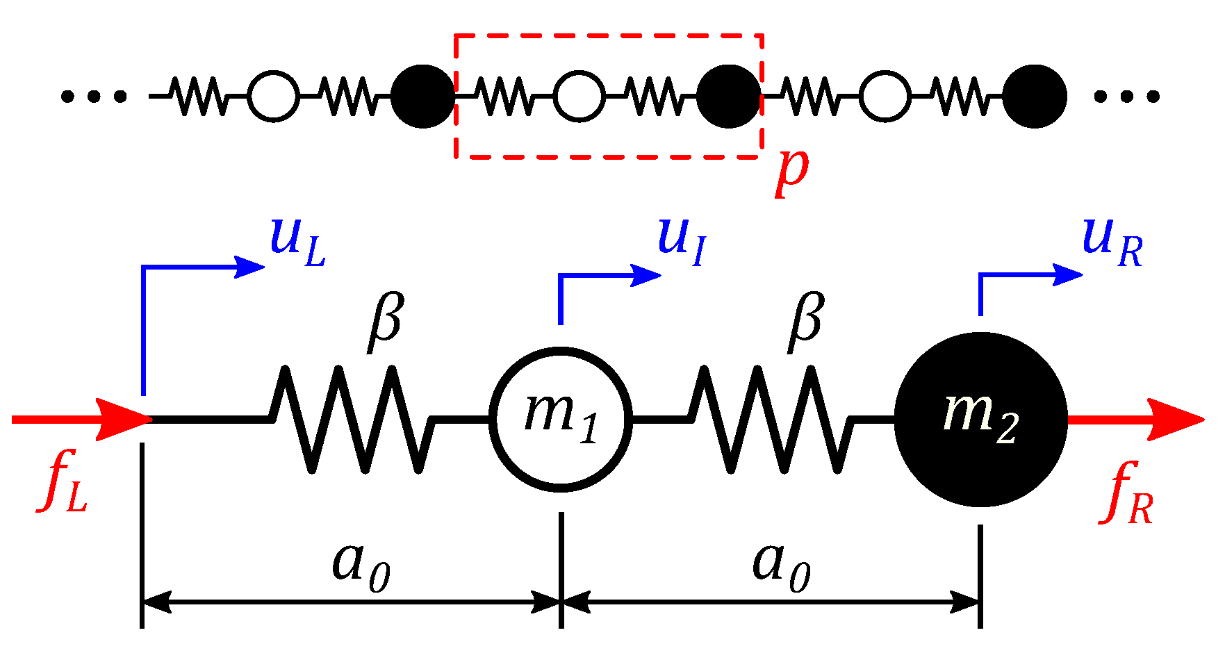
As shown in Figure 1, the 1D viscoelastic diatomic lattice is characterized by a unit cell with masses $m_1$ and $m_2$, separated by distance $a_0$ and connected by springs with stiffness $\beta$. Thus, the lattice constant a is $2a_0$. To validate the indicator for damped as well as undamped systems, the springs are assumed to be viscoelastic, with the spring stiffness characterized by a complex number $\beta ={\beta }_0{e}^{i\delta }$, where ${\beta }_0$ is the magnitude of the spring stiffness and the loss angle $\delta$ is varied to control the dissipation of the lattice without changing the spring stiffness. $\delta =0$ corresponds to an undamped lattice.

We use the transfer matrix method to solve for the dispersion relation of the lattice. The transfer matrix links the left boundary forces and displacements from the pth unit cell to the $p+1$ unit cell according to

$$\begin{array}{c}\hfill \left[T\right]{\left\{\begin{array}{c}{u}_L\\ f_L\end{array}\right\}}^{\left(p\right)}={\left\{\begin{array}{c}{u}_R\\ -f_R\end{array}\right\}}^{\left(p\right)}={\left\{\begin{array}{c}{u}_L\\ f_L\end{array}\right\}}^{(p+1)},\end{array}$$

(19)

where $u_L$ ($u_R$) and $f_L$ ($f_R$) are the displacements and forces, respectively, on the left (right) side of the unit cell, and

$$\begin{array}{c}\hfill \left[T\right]=\left[\begin{array}{cc}1-\frac{{\omega }^2{m}_1}{\beta }& \frac{2\beta -{\omega }^2{m}_1}{{\beta }^2}\\ -\frac{{\omega }^4{m}_1{m}_2-\beta {\omega }^2(m_1+m_2)}{\beta }& \frac{{\omega }^4{m}_1{m}_2-\beta {\omega }^2(m_1+2m_2)+{\beta }^2}{{\beta }^2}\end{array}\right]\end{array}$$

(20)

is the transfer matrix. We prescribe real frequencies $\omega$ and compute the complex wavenumber k and mode shapes $\widehat{u}$ from the eigenvalues and eigenvectors of the transfer matrix. We use the PBME method to determine the modal amplitudes and compute the evanescence indicator. For the purposes of illustration, we choose $m_1=1$, $m_2=2$, ${\beta }_0=1$, $a_0=0.5$, and an input displacement amplitude $u_0=0.01$. All results are presented in terms of the normalized angular frequency $\omega /{\omega }_0$, where ${\omega }_0=\sqrt{2{\beta }_0/m_2}$ is the lower edge frequency of the first band gap for the undamped PC. We vary the parameters $\delta$, N, and $u_{thres}$ to study their effect on the computed evanescence indicator and the fuzzy band gaps. All results are presented in terms of normalized transmission amplitudes $T=u\left(Na\right)/u_0$ and $T_{thres}=u_{thres}/u_0$. To verify that the true displacement at unit cell N is accurately captured by a summation of Bloch modes with the computed modal amplitudes, we also compute the true response of the finite structure by constructing the dynamic stiffness matrix including all degrees of freedom, applying appropriate boundary conditions, and inverting the dynamic stiffness matrix.

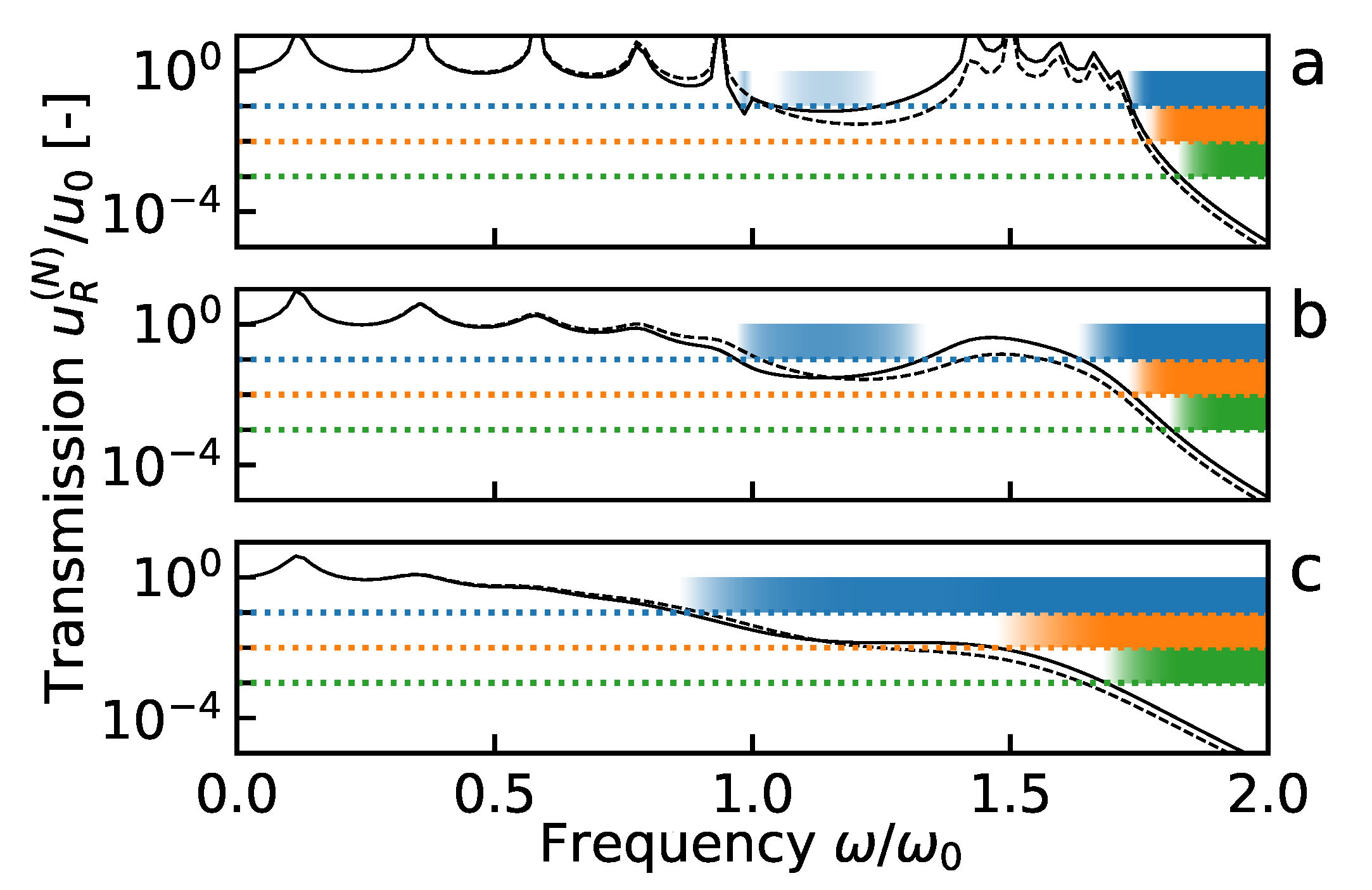
The evanescence indicator is shown in Figure 2 for a finite structure of reference with $N=5$. In each plot (a–c), the effect of the threshold displacement amplitude $u_{thres}$ on the fuzzy band gaps is shown by varying $u_{thres}={10}^{-3},{10}^{-4},{10}^{-5}$, which corresponds to threshold transmission amplitudes $T_{thres}={10}^{-1},{10}^{-2},{10}^{-3}$, respectively. The $T_{thres}$ values are plotted as horizontal dashed lines and per the generalized fuzzy band gap definition, a fuzzy band gap is defined to exist at any frequency where the evanescence indicator falls below $T_{thres}$. As in [22,24], we use a shading model to visualize the evanescence indicator. In our model, regions with transmission $T > T_{thres}$ are shaded white, indicating that no fuzzy band gap exists at that frequency. Regions with transmission $T < 0.1T_{thres}$ are shaded with a solid color, and intermediate values $0.1T_{thres} < T <T_{thres}$ are assigned shades between white and the solid color, so that shaded bars indicate the fuzzy band gaps. This luminance-based shading scheme is an intuitive choice for representing relative values of data [38], and it enables ready visual identification of band gaps while also illustrating how the wave amplitude progresses through smooth transitions near the fuzzy band gap edges. If the threshold value is based on an engineering requirement, such as the maximum allowable vibration amplitude in a structure, the “darkness” of the shading can be interpreted as the factor of safety of the system against the given requirement. White regions indicate a factor of safety of 1 or less, dark regions indicate a factor of safety of 10 or more, and intermediate shades indicate a factor of safety between 1 and 10. The shading near the fuzzy band gap edges is reminiscent of out-of-focus photos due to the lack of sharp contrast. This gives rise to the moniker “fuzzy band gaps”, as out-of-focus photos are often colloquially described as “fuzzy”.

From Figure 2, it is evident that the existence of fuzzy band gaps is dependent on the selected value of $T_{thres}$. For example, in panel (a), a fuzzy band gap exists between 1.05–1.24${\omega }_0$ for $T_{thres}={10}^{-1}$ because the evanescence indicator (black dashed line) falls below $T_{thres}={10}^{-1}$ (blue dotted line) in that frequency range. However, when the threshold transmission is selected as $T_{thres}={10}^{-2}$ or $T_{thres}={10}^{-3}$, there is no fuzzy band gap, because the trough in the evanescence indicator is not deep enough to reach $T_{thres}={10}^{-2}$ or $T_{thres}={10}^{-3}$ (orange and green dotted lines). The existence/nonexistence of fuzzy band gaps is also readily apparent from the shaded bars, as the light blue shaded region between 1.05–1.24${\omega }_0$ indicates a fuzzy band gap, while the lack of any orange or green shading in the same frequency range shows that no fuzzy band gap exists for those threshold amplitudes.

In addition to determining the existence of fuzzy band gaps, the threshold amplitude also affects the frequencies at which fuzzy band gaps occur. For example, in panel (a), the edge of the high-frequency fuzzy band gap increases in frequency from 1.74${\omega }_0$ to 1.77${\omega }_0$ to 1.83${\omega }_0$ as $T_{thres}$ is varied from ${10}^{-1}$ to ${10}^{-2}$ to ${10}^{-3}$, as determined by locating the intersection of the evanescence indicator curve with the horizontal dotted lines that indicate the selected threshold amplitudes. This gives the shaded bars a stair-step appearance.

Figure 2 also reveals how the loss factor $\delta$ affects the existence, position, and width of the fuzzy band gaps. Conferring with Figure 2a for the undamped case, it can be seen that a fuzzy band gap exists between 1.05 and 1.24${\omega }_0$. As the dissipation in the lattice is increased to $\delta =0.1$, the width of the fuzzy band gap increases to 0.97–1.33${\omega }_0$. The trough is deeper than for the undamped case, so the structure of reference meets the threshold amplitude with a greater margin, and thus the shading is darker than for the undamped fuzzy band gap. However, the trough is still not sufficiently deep to meet the $T_{thres}={10}^{-2},{10}^{-3}$ threshold amplitudes, and so a fuzzy band gap is not formed for those cases. As the dissipation is further increased by increasing the loss factor to $\delta =0.3$ (Figure 2c), the two fuzzy band gaps which existed for the $T_{thres}={10}^{-1}$ case merge into a single high-frequency fuzzy band gap starting at 0.86${\omega }_0$. This is the result of the disappearance of the optical pass band, which is much more strongly affected by damping than the acoustic pass band [14]. The disappearance of the optical pass band causes a large decrease in the edge frequency of the single fuzzy band gap identified for $T_{thres}={10}^{-2}$ and $T_{thres}={10}^{-3}$. Finally, it is apparent that the fuzzy band gaps become “fuzzier” with increasing dissipation, that is, the shaded transition from white to solid color becomes wider as the dissipation is increased. This is a result of the slope of the evanescence indicator curve near the fuzzy band gap edges becoming less steep with increasing dissipation. This, in turn, is caused by increasingly smooth transitions in the $k_I$ band structure as $\delta$ is increased.

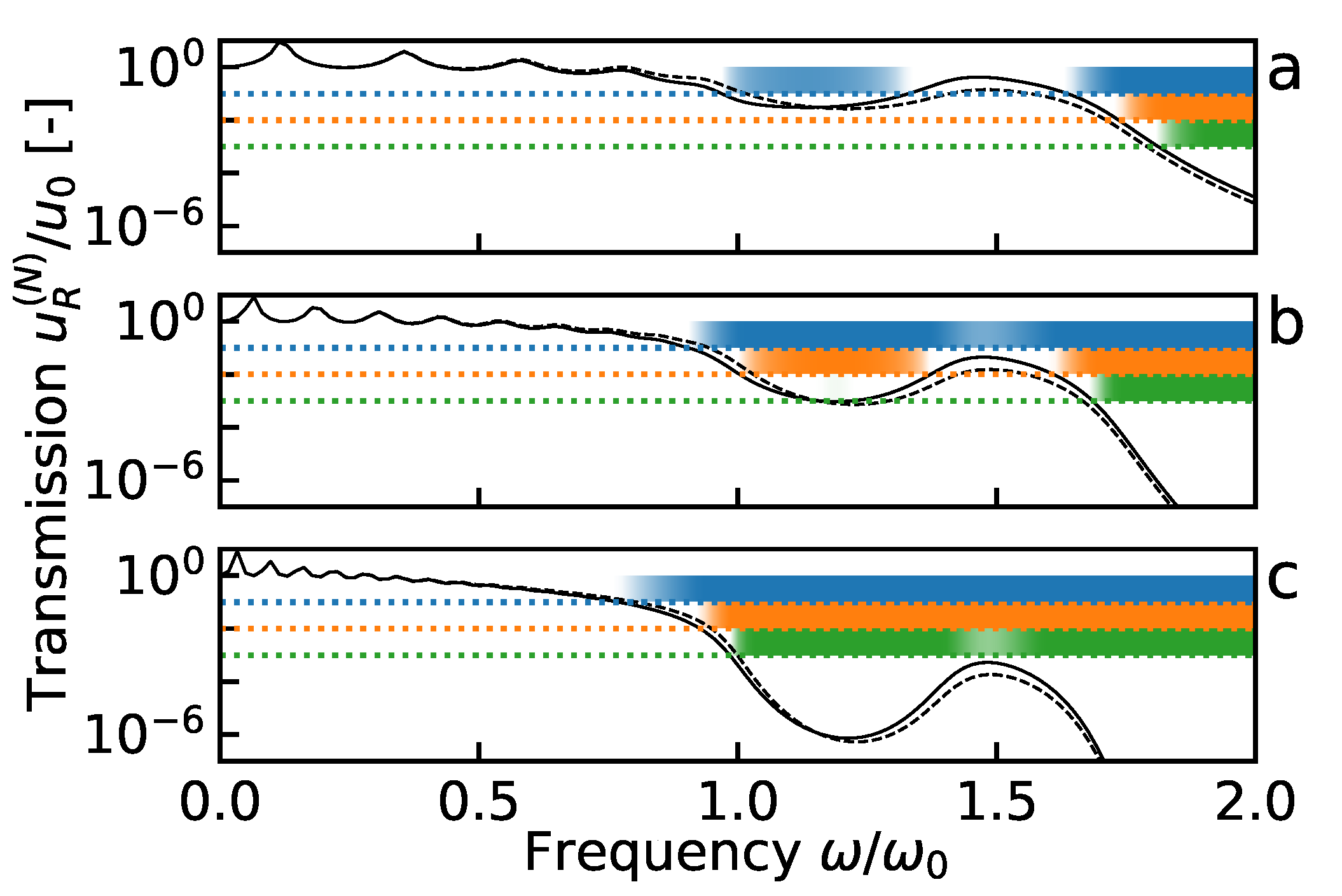
Figure 3 shows how the number of unit cells N in the finite structure of reference affects the fuzzy band gaps. For $N=5$ (Figure 3a), there are two fuzzy band gaps when $T_{thres}={10}^{-1}$ and only one fuzzy band gap when $T_{thres}={10}^{-2}$ and ${10}^{-3}$, as discussed previously. However, when N is increased to 10 (Figure 3b), the two fuzzy band gaps observed for $T_{thres}={10}^{-1}$ merge into a single fuzzy band gap, while for $T_{thres}={10}^{-2}$, a new fuzzy band gap opens between 1.0–1.37${\omega }_0$. This behavior is expected, as the additional length of the $N=10$ structure of reference allows for a greater loss of amplitude by the decaying waves as they propagate [32,33]. Figure 3b also illustrates an interesting feature of the shading approach: the ability to identify near-passbands. Though the $N=10$ structure exhibits a single fuzzy band gap for all frequencies greater than 0.9${\omega }_0$ when $T_{thres}={10}^{-1}$, the peak in the evanescence indicator at 1.47${\omega }_0$ nearly reaches the threshold amplitude. This is visualized by a region of lighter blue color centered around 1.47${\omega }_0$. The same phenomenon is observed for $N=20$ and $T_{thres}={10}^{-3}$ in Figure 3c. Finally, it is observed that increasing N tends to decrease the “fuzziness” of the fuzzy band gaps, because the wave attenuation is magnified by the increased number of unit cells, resulting in steeper rolloffs at the fuzzy band gap edges.

To confirm the accuracy of the propagated Bloch mode expansion method, we compare the evanescence indicator with the true displacement of the N-cell finite structures, computed using the full set of dofs for the finite structure. For each case of $\delta$ and N in Figure 2 and Figure 3, the normalized displacement amplitude for mass $m_2$ of cell N is plotted with a black dashed line. In general, the evanescence indicator agrees with the true displacement within half a decade or less. The agreement is nearly perfect for frequencies less than 0.75${\omega }_0$ in all cases, with the largest deviation observed in the frequency range of the optical mode. The deviation decreases as the loss factor is increased, with a maximum deviation of 5.9 dB for $N=5$ and $\delta =0.3$, compared to a maximum deviation of 21.2 dB for $N=5$ and $\delta =0.0$. Interestingly, the deviation between the evanescence indicator and the true displacement is almost unaffected by changing the number of unit cells N, with a maximum deviation of 10.1dB for each of the cases shown in Figure 3. At first glance this seems counterintuitive, as the PBME method applied to this system essentially consists of reducing a $(2N+1)$-dof structure to two dofs, and increasing N therefore results in a greater reduction in the number of dofs, which would be expected to give a worse approximation. However, increasing the number of dofs in the finite structure causes its dynamics to more closely resemble the dynamics of the infinite system, making the Bloch modes more closely resemble the modes of the finite structure. These competing effects appear to cancel out, allowing the PBME method to model arbitrarily large structures with only two dofs.

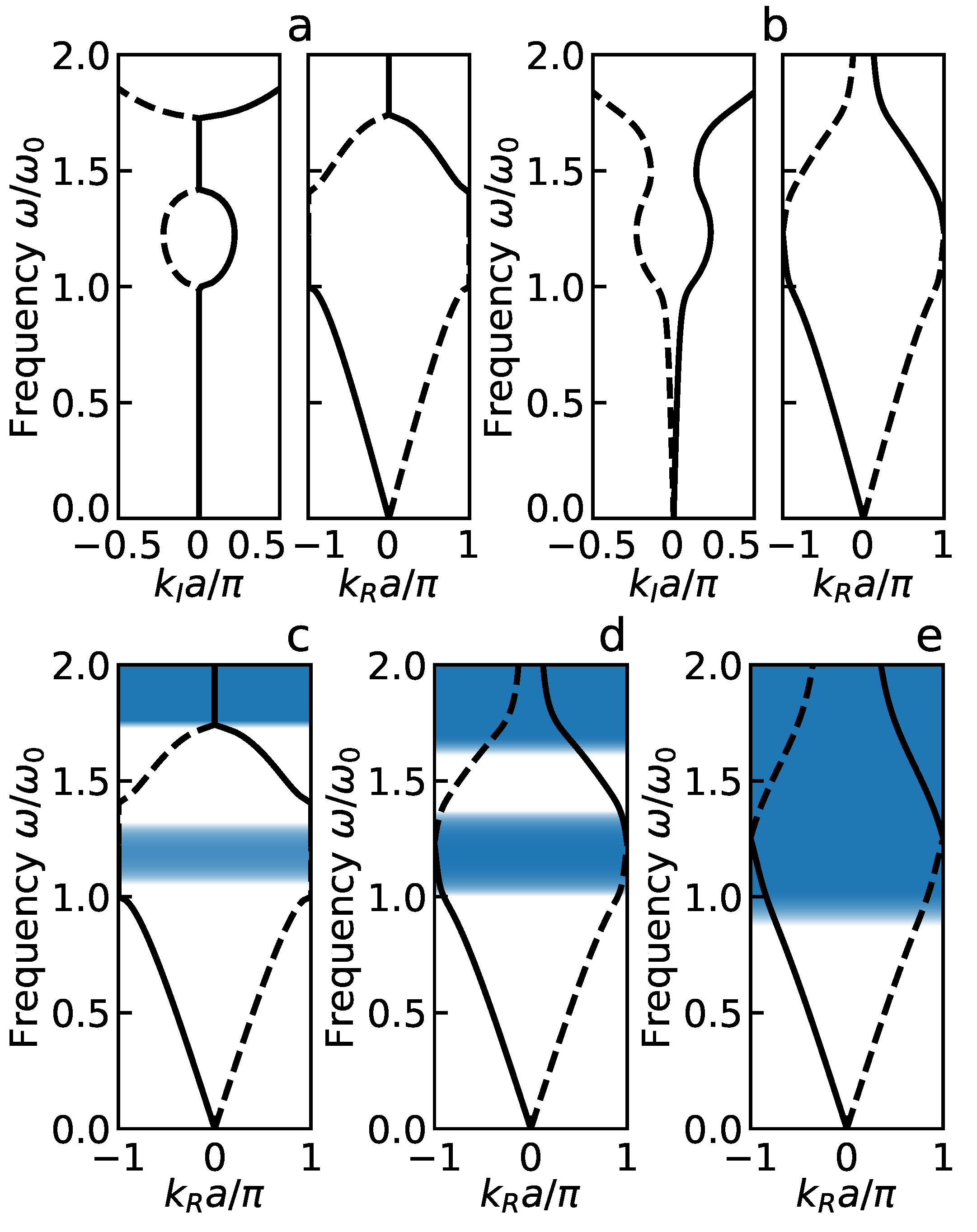
Figure 4 illustrates how the evanescence indicator and fuzzy band gap shading can be used to simplify the presentation and interpretation of damped dispersion relations. For the undamped lattice (Figure 4a), the band gaps can be easily identified using either of two methods: by locating frequency ranges where $k_R$ is 0 or $\pi /a$, or by locating frequency ranges where $k_I$ is nonzero. However, the introduction of damping changes the eigenmodes and causes the band gap to close (Figure 4b), as the acoustic and optical modes for $k_R$ are no longer distinct but instead meet at the edge of the first Brillouin zone, and $k_I$ is nonzero for all frequencies. This has been noted before in the literature, see, e.g., in [12]. In the damped case, it is thus necessary to present both the real and imaginary parts of the wavenumber to understand the wave propagation behavior.

In contrast with the complicated picture of wave propagation painted by Figure 4a,b, Figure 4c–e provides a much clearer picture of the wave behavior. The evanescence indicator is computed for $N=10$, $T_{thres}={10}^{-2}$ for three different loss factors, and the fuzzy band gap shading is plotted directly on the dispersion relation using the same shading model as in Figure 2 and Figure 3. The fuzzy band gaps are clearly visible from the shaded regions, even for the damped lattices where the fuzzy band gap edges cannot be inferred from the dispersion curves alone (Figure 4d,e). In addition, it is not necessary to present the imaginary part of the wavenumber to give a clear picture of the wave propagation behavior because the essential information about the decay of the wave amplitude is captured by the fuzzy band gap shading, which reduces the complexity of the figure. Interestingly, the fuzzy band gap identified by the evanescence indicator for the undamped lattice (shaded region in Figure 4c) is noticeably narrower than the band gap identified by the traditional means (which exists between ${\omega }_0$ and $\sqrt{2}$${\omega }_0$). This can be explained by referring to the imaginary part of the wavenumber shown in Figure 4a. Near the edges of the band gap, $k_I$ is close to 0, which gives a slow spatial decay that is not sufficient to cause the transmission to fall below $T_{thres}$ within $N=5$ unit cells. The evanescence indicator thus provides a more practical assessment of the effectiveness of the lattice for suppressing vibrations than the traditional method of identifying band gaps.

4. Example 2: Magneto-Active Metastructures

We now apply the evanescence indicator to a damped PC with a complex 3D geometry: a magneto-active metastructure. These structures were studied in [11], and are based on a unit cell which consists of a lattice surrounding a large included mass. The metastructure is composed of magneto-active elastomer (MAE), a smart material composed of magnetic particles in a non-magnetic elastomer matrix which exhibits an increase in modulus in the presence of a magnetic field [39,40]. Prior work showed that the tunable modulus enabled the metastructure to exhibit a magnetically-tunable, longitudinally-polarized band gap [11]. For more details on the geometry of these structures and their magnetic tunability, the reader is referred to the prior article [11]. In the present work, we show that the evanescence indicator is able to accurately predict the longitudinally-polarized band gaps shown in [11], as well as flexural and torsional band gaps that have not been previously studied.

4.1. Materials and Methods

The MAE metastructures studied in [11] used a direct-ink write additive manufacturing process to fabricate metastructures in two geometries with different lattice configurations, termed “low-stiffness” and “mid-stiffness”. In the present work, for simplicity of presentation we include results only for the low-stiffness geometry described in [11], but the method is also applicable to the mid-stiffness geometry. The MAE consisted of spherical carbonyl iron particles ($3\mathsf{\mu }\mathrm{m}$ average diameter, US1163M; US Research Nanomaterials, Houston, TX USA) and poly(dimethylsiloxane) (PDMS) elastomer (Sylgard 184; Dow Corning, Midland, MI USA) combined in an 8:1 weight ratio. Using a mixture rule, we computed the MAE density $\rho$ to be 4500 kg/m³. Prior dynamic compression experiments on cylindrical samples of MAE characterized the frequency-dependent complex modulus $E^{*}\left(\omega \right)=E^{\prime }\left(\omega \right)+i{E}^{″}\left(\omega \right)$, and the following curve fits were extracted [11].

$$\begin{array}{c}\hfill E^{\prime }\left(\omega \right)=1.73\times {10}^4\omega +2.76\times {10}^7\mathrm{Pa}\\ \hfill E^{″}\left(\omega \right)=6.27\times {10}^3\omega +8.95\times {10}^6\mathrm{Pa}\end{array}$$

(21)

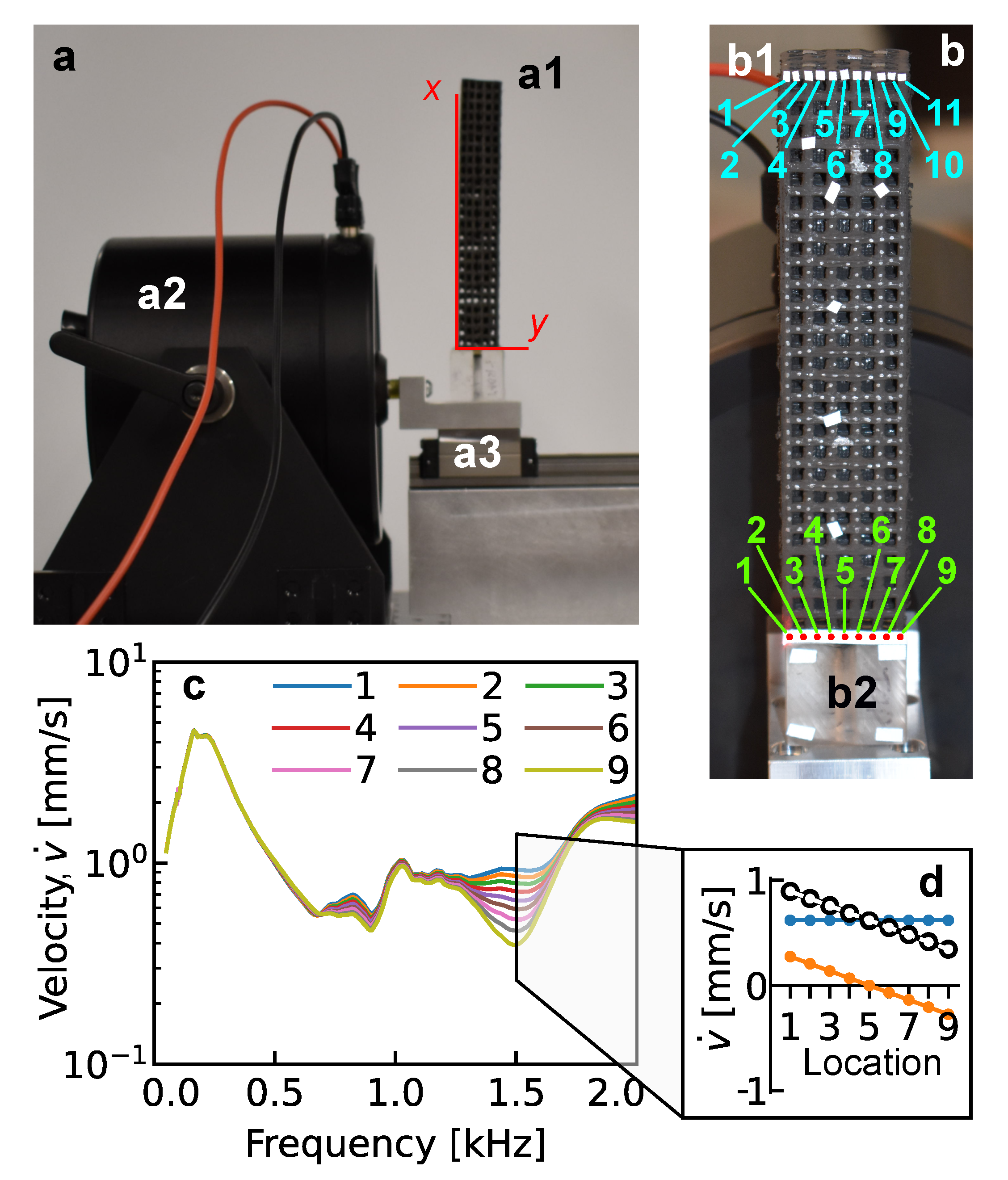
To compute the band structure of the MAE metastructures, we use two approaches. First, we repeat the results in [11], in which we used an indirect $\omega \left(k\right)$ FEM approach which was modified to include the frequency dependence of the complex modulus $\left|E^{*}\left(\omega \right)\right|=\sqrt{E^{\prime }{\left(\omega \right)}^2+E^{″}{\left(\omega \right)}^2}$ but neglected viscoelasticity. In the present work, we use the band structure obtained in [11] and study fuzzy band gaps with respect to three different wave polarizations: “longitudinal” waves with displacements primarily in the x-direction, “flexural” waves with displacements primarily in the y-direction that resemble beam bending, and “torsional” waves with displacements resembling rotations about the x-axis. To identify the polarized band gaps, we compute the MPF for the polarization of interest for each mode, and manually select the subset of modes for which the MPF is greater than half of the maximum MPF for that polarization. From the chosen subset of modes, we identify band gaps for the polarization of interest. This method was used in [11] to identify longitudinal band gaps. In this article, we further use this method to identify flexural band gaps and henceforth refer to it as the “MPF inspection method”. To compute the damped band structure, we use a direct $k\left(\omega \right)$ FEM approach following the method of [24], which considers both the frequency dependence and damping of the MAE through the complex modulus (Equation (21)). The $k\left(\omega \right)$ method is implemented by modifying the standard eigenvalue formulation of a commercial FEM software package (COMSOL Multiphysics). The COMSOL model files for the modified formulation are provided in the publicly available dataset that accompanies this article. We extract the Bloch wavenumbers k and mode shapes $\widehat{\mathit{u}}\left(\mathit{x}\right)$ from the FEM solution and compute the evanescence indicator to determine the fuzzy band gaps. To compute the evanescence indicator for longitudinally-polarized waves, we choose the input and output as the x-component of displacement, with the input taken at a single point on the $x=0$ face of the metastructure, and the output taken at a single point on the opposite face. The points are taken at the same location as the point selected for the experiments and simulations in [11]. To compute the evanescence indicator for flexurally-polarized waves, we choose the input as the average y-displacement of nine points and the output displacement as the average y-displacement of 11 points as shown in Figure 5b.

To experimentally verify the evanescence indicator, we characterized the band gaps in the metastructures by performing vibration transmission measurements on the finite metastructure specimen ($N=5$) fabricated in [11]. In [11], we characterized longitudinal band gaps using an electrodynamic shaker (Model 4810; Brüel and Kjær, Nærum, Denmark) to excite longitudinal vibrations in the metastructure in a forced-free configuration, and measured the out-of-plane (x) velocity at both ends of the metastructure using a laser Doppler vibrometer (Model OFV-5000 with OFV-505 single point laser head; Polytec, Waldbronn, Germany) and lock-in amplifier (Model SR830; Stanford Research Systems, Sunnyvale, CA USA). We computed vibration transmission as the ratio of the output and input velocities. The experimental results for longitudinal excitation are taken from the work in [11], and complete details of the experimental setup for longitudinal waves can be found in that article.

In the present work, we also characterized hybrid flexural-torsional band gaps using the frequency sweep bending setup of the work in [29]. We attached the metastructure (Figure 5(a1)) to an acrylic block using two-part epoxy adhesive, and then attached the acrylic block to a linear guide (Figure 5(a3)) to allow translations in the y-direction. The acrylic block was attached to the linear guide with a single screw at the center axis of the block, which allowed the block to rotate about an axis parallel to the x-axis. The displacement imparted to the metastructure by the acrylic block thus consisted of a superimposed translation and rotation. The linear guide was excited with harmonic displacements using an electrodynamic shaker (Model 4809; Brüel and Kjær, Nærum, Denmark, see Figure 5(a2)), and the out-of-plane (y-direction) velocity $\dot{v}$ of the metastructure was measured using a laser Doppler vibrometer (Polytec OFV-5000). The “input” velocity was taken as the average of nine points on the acrylic block (Figure 5(b2)) and the “output” velocity was taken as the average of 11 points on the free end of the metastructure (Figure 5(b1)). To characterize the frequency response of the input translation and rotation, we decomposed the input mode shape (formed by the nine input velocities; see Figure 5c) into its constituent translation and rotation (Figure 5d) for each frequency studied.

To further verify the evanescence indicator, we computed the vibration transmission through an $N=5$ cell finite structure using FEM simulations. The viscoelastic and dynamic properties of the MAE were modeled using the density $\rho$ and complex modulus $E^{*}\left(\omega \right)$ obtained for the real MAE material. For longitudinal excitation, we take the results in [11], which were obtained by prescribing a uniform displacement in the x-direction on the input ($x=0$) face of the metastructure and measuring the output displacement at the same point on the metastructure as in the experiments. In the present work, we set up the FEM model in a similar fashion to study flexural, torsional, and flexural-torsional excitation. Instead of x-displacements, we prescribe displacements on the input face of the metastructure that are appropriate to each polarization: uniform y-displacement for flexural waves, rotation in the $yz$-plane about the center of the $x=0$ face for torsional waves, and y-translation plus $yz$-rotation for flexural-torsional excitation. For the flexural, torsional, and flexural-torsional simulations, we computed the input and output displacements in the same way as the experiments: by averaging the displacement amplitude over the input and output points shown in Figure 5b. We study the fuzzy band gaps only for $N=5$ as the specimen used in the experiments consists of $N=5$ unit cells, but it is expected that the MAE metastructure fuzzy band gaps will exhibit a similar dependence on N as the diatomic lattice.

4.2. Results

The damped and undamped dispersion relations for the MAE metastructure are shown in Figure 6 and Figure 7. Figure 6a and Figure 7a present the damped dispersion relation, while Figure 6b and Figure 7b present the undamped dispersion relation. Comparing the damped dispersion relation to the undamped dispersion relation shows the effect of damping on the band structure. Each of the undamped dispersion curves (Figure 6b) starts and ends at the edges of the first Brillouin zone ($k=0$ and $k=\pi /a$) and all wavenumbers are real. Each dispersion curves exists only over a limited frequency interval, so it is possible to identify band gaps that lie between the upper frequency of one Bloch mode and the lower frequency of another. In contrast, the damped dispersion curves (Figure 6a) do not have frequency limits; each curve exists over all frequencies and therefore it is not possible to identify band gaps in the usual manner. Furthermore, all wavenumbers are complex (rather than real as in the undamped case), with the real ($k_R$) and imaginary ($k_I$) parts of the wavenumber shown on separate axes in Figure 6a and Figure 7a. As the MAE metastructure admits Bloch wave modes with many polarizations, the relevant modes are identified by computing the MPF for each Bloch mode shape and coloring the dispersion curves accordingly. The modes colored yellow or green in Figure 6a,b and Figure 7a,b have strong longitudinal and transverse polarizations, respectively, while modes colored blue or purple are not significant to those polarizations.

4.2.1. Undamped Band Gaps

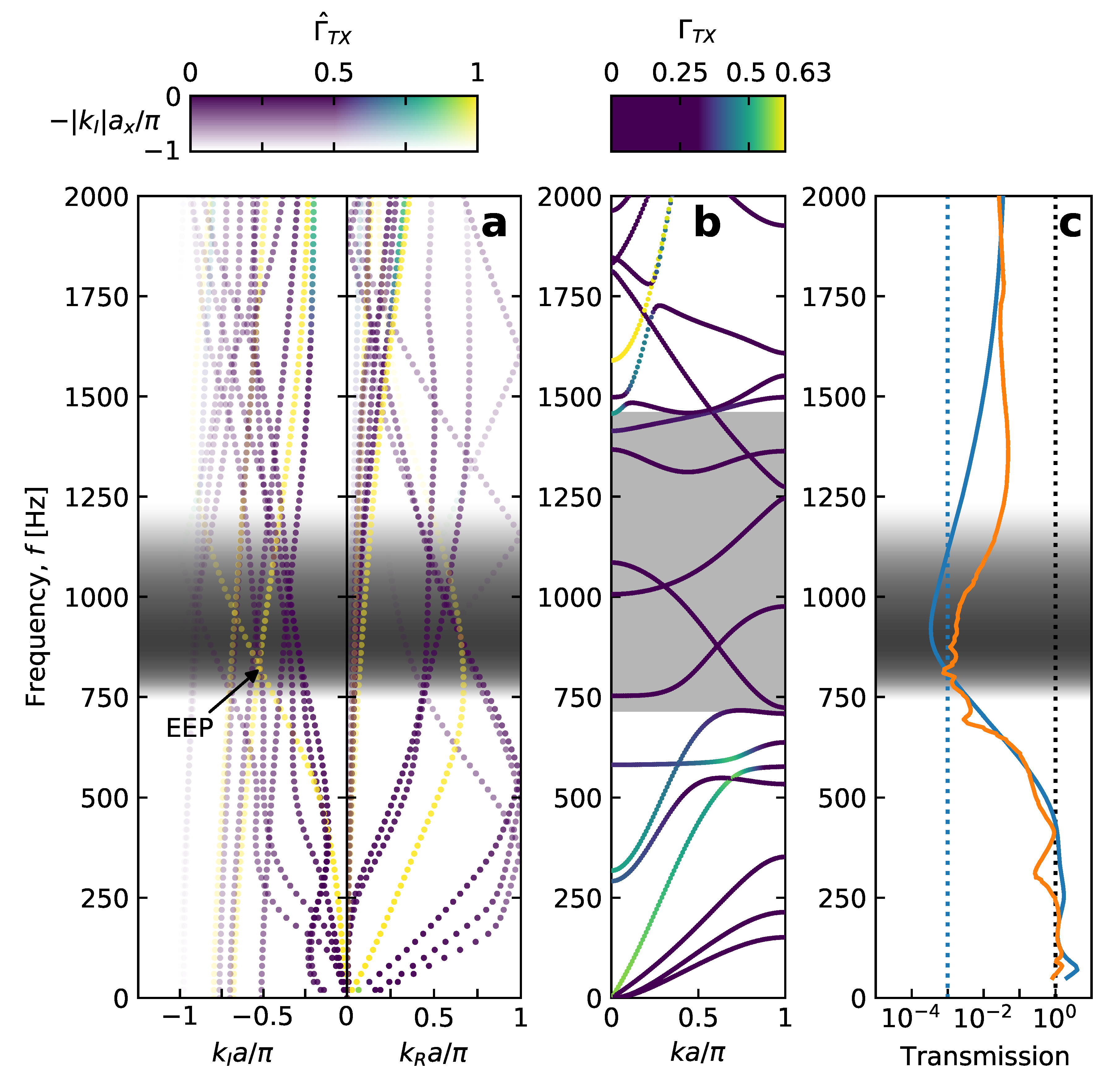
Figure 6 presents the results for longitudinally-polarized waves. The undamped dispersion relation and the experimental and simulated transmission reported in [11] are shown in Figure 6b,c. It is clear that the experimental band gap is a polarized band gap, as the only complete band gap in the dispersion relation (near 1250 Hz) is very narrow and higher in frequency than the experimental band gap. The MPF inspection method is used to identify the longitudinal band gap. Each data marker in Figure 6b is colorized by ${\Gamma }_{TX}$, and the shading is chosen so that modes which do not meet the criteria for a longitudinal mode (i.e., ${\Gamma }_{TX}$ less than half the maximum value; ${\Gamma }_{TX}<0.315]$) are colored dark purple. From the subset of longitudinal modes (those with blue-green-yellow coloration), a longitudinally-polarized band gap between 717 and 1457 Hz (Figure 6b) is found, which approximately corresponds with the experimental band gap. The low-frequency edge of the band gap in Figure 6b exhibits very good agreement with the low-frequency edge of the transmission trough for both the experimental and simulated transmissions in Figure 6c. However, the undamped band gap is much wider (740 Hz) than the width of the experimental transmission trough (approximately 400 Hz). As damping strongly affects the real part of the dispersion relation [12], the undamped band structure is not expected to be a good predictor of the behavior of the damped MAE metastructure. This suggests that the overlap of the undamped longitudinal band gap and the experimental transmission trough may be purely coincidental.

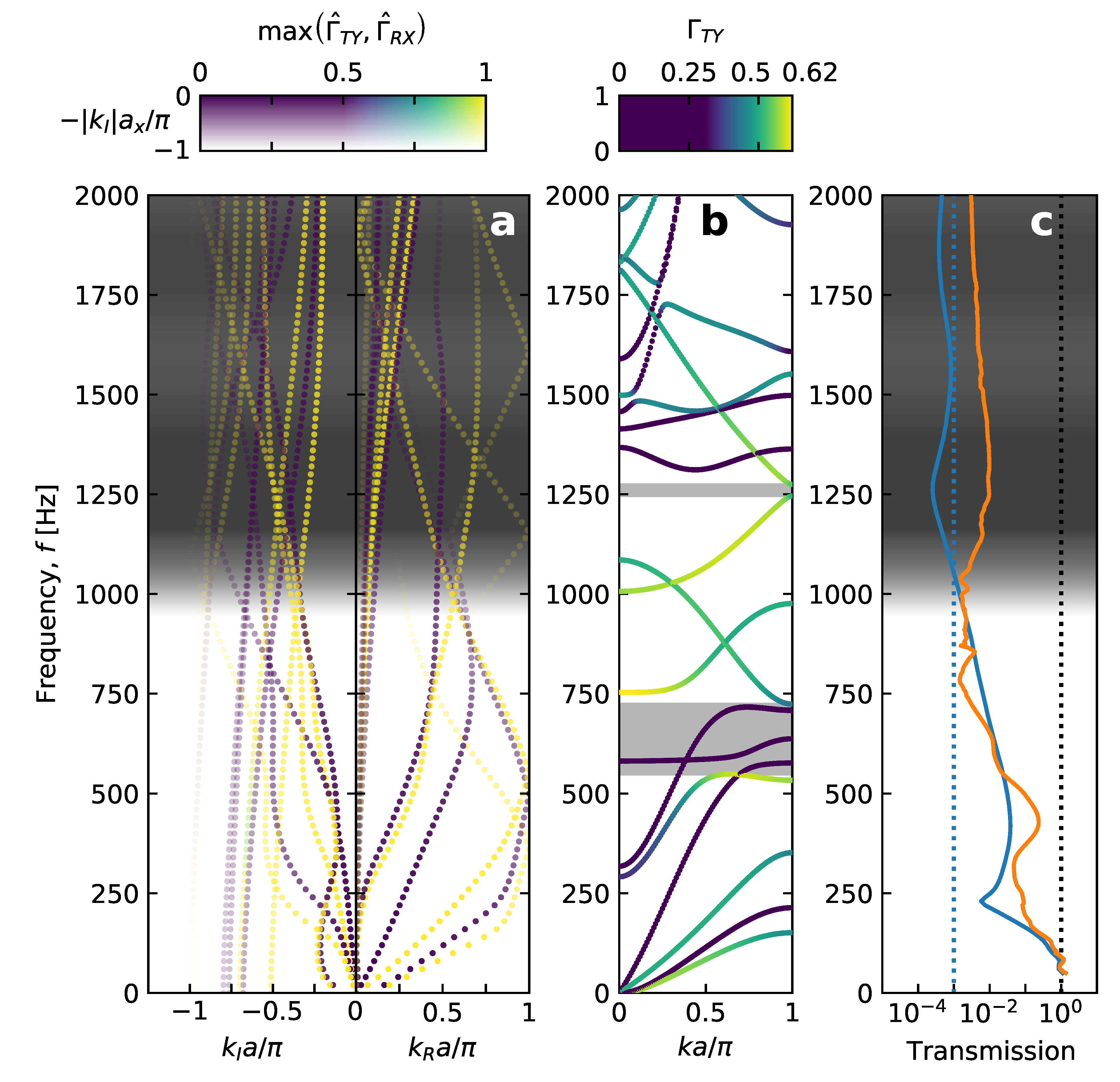
This notion is further supported by the complete lack of correspondence between the undamped band gaps and experimental results for other polarizations. In particular, no such correspondence is observed for flexural-rotational excitation (Figure 7b,c). The undamped dispersion relation of Figure 6b is repeated in Figure 7b, but in Figure 7b the colorization of the modes is based on ${\Gamma }_{TY}$ rather than ${\Gamma }_{TX}$ to highlight flexurally-polarized waves. To identify flexural band gaps, all modes colored dark purple in Figure 7b are ignored and gaps are sought between the remaining modes. This process gives two band gaps at 549–724 Hz and 1246–1274 Hz. The wider of these band gaps is lower in frequency than the longitudinal band gap, which is in keeping with the observations in [27] for similar geometries. Above 724 Hz, there are modes with significant flexural polarization everywhere except in the narrow band gap at 1246 Hz, which indicates that the metastructure should transmit flexural waves at high frequencies. However, the experimental and simulated transmission show that the opposite is true: the metastructure attenuates flexural waves above 1000 Hz. This contradiction between the undamped band gap and experimental results shows that the undamped MPF inspection method cannot reliably predict polarized band gaps in damped systems. We therefore reiterate the importance of considering damped band structures when comparing with experimental results. As we show next, applying the MPF inspection method to the damped band structure raises several challenges, which illustrates the utility of the evanescence indicator.

4.2.2. Damped MPF Inspection Method

Figure 6a and Figure 7a show the damped band structure for the MAE metastructures, from which the limitations of the MPF inspection method for damped band structures are evident. In Figure 6a, the data markers are colored to highlight longitudinally-polarized waves, while in Figure 7a the data markers are colored to indicates modes with either a flexural or rotational polarization. In each of these figures, the normalized MPF $\widehat{\Gamma }$ is used instead of the non-normalized MPF $\Gamma$, because $\Gamma$ is much smaller at high frequencies than at low frequencies due to the decay of the high-frequency waves. Using $\Gamma$ for the marker color would thus give the erroneous impression that there are no longitudinally-polarized modes at high frequencies, and therefore $\widehat{\Gamma }$ is a better polarization indicator. Furthermore, the process of normalizing ${\Gamma }_{\mathit{T}}$ and ${\Gamma }_{\mathit{R}}$ removes the scaling difference between the rotational and translational MPFs (Section 2.4.2) so that they can be compared. Figure 6a shows that there are three modes (shown in yellow) with a significant longitudinal polarization. In addition, there is a fourth mode ($k_I\approx 0.2\pi /a$ at 2000 Hz) for which the longitudinal polarization is not significant at low frequencies but becomes significant above 1750 Hz, as evidenced by the data points turning green above 1750Hz. Each of these four dispersion curves is smooth and continuous across the range of frequencies studied, exhibiting no band gaps.

At low frequency, longitudinal wave transmission is dominated by a single mode ($k_R\approx 0.5\pi /a$ at 500 Hz), the longitudinal “resonator” mode with displacements concentrated in the large included mass. The other three longitudinal modes are purely evanescent ($k_R=0$, $k_I\ne 0$) at $\omega =0$ and strongly decaying at low frequencies, having much larger $|k_I|$ than the resonator mode. In undamped systems, such modes are purely evanescent below a cut-off frequency and become propagating modes above the cut-off frequency, and can be physically likened to “frustrated diffracted waves” in diffraction gratings [26]. In damped systems such as the MAE metastructures, the wavenumber for these “frustrated modes” takes on a nonzero real part for all $\omega >0$, although the modes remain strongly decaying at low frequencies [12] and thus have a negligible contribution to wave transmission. However, they become more propagative at higher frequencies than at low frequencies, due to their increasing $k_R$ and decreasing $k_I$. Conversely, the resonator mode, which is initially propagative, becomes more evanescent at high frequency than at low frequency, with an especially rapid increase in $|k_I|$ occurring above 500 Hz. This eventually causes the frustrated modes to usurp the resonator mode as the dominant contributors to longitudinal wave transmission. The “equal evanescence point” (EEP), defined as the frequency where $k_I$ is equal for both the resonator mode and the frustrated mode, occurs at about 820 Hz, as shown in Figure 6a. This falls within the experimental and simulated transmission troughs shown in Figure 6c, which suggests that this type of “dominant-mode transition” is responsible for the emergence of fuzzy band gaps in damped PCs. To aid in identifying dominant-mode transitions, the transparency of each data point is made proportional to the imaginary part of the wavenumber. This makes highly evanescent waves appear faint, indicating that their contribution to the total transmitted wave amplitude is insignificant. Increases in $|k_I|$ are represented by transitions from opaque to transparent data markers, making modes “disappear”, as, for example, the resonator mode above 1150 Hz. The results for flexural-torsional modes (Figure 7a) exhibit many of the same features as for longitudinal modes, including mode appearance and disappearance and dominant-mode transitions. Due to the inclusion of both flexural and torsional modes, a larger subset of modes are identified as significant than in the longitudinal case, as evidenced by the larger number of dispersion curves highlighted in yellow in Figure 7a than in Figure 6a.

The damped MPF inspection method of prescribing marker color and transparency is useful as a heuristic illustration of the features of a damped band structure that govern fuzzy band gap formation in damped PCs, but is less useful as a quantitative measure of the fuzzy band gap frequencies. The coloration of each data marker, which classifies a mode as significantly or not significantly polarized in the direction of interest, is dependent on an arbitrary parameter: the threshold value of $\widehat{\Gamma }$. Likewise, the transparency of each marker, which indicates the decay of each wave mode, is also affected by an arbitrary parameter: the value of $|k_I|$ which is assigned to be fully transparent (chosen as $|k_I|=\pi /a$ in Figure 6a and Figure 7a). Additionally, using the normalized MPF $\widehat{\Gamma }$ as an indicator of wave polarization removes the possibility of comparing the relative amplitudes of different modes at the same frequency.

4.2.3. Evanescence Indicator: Longitudinal Fuzzy Band Gaps

In light of these limitations of the damped MPF inspection method, the utility of the evanescence indicator becomes apparent. Using the MPF for translations in the longitudinal (x) direction (${\Gamma }_{j,TX}$) to compute the modal amplitudes $A_j$, and considering an $N=5$ finite structure of reference, we compute the evanescence indicator for longitudinal excitation. Choosing $T_{thres}={10}^{-3}$, we plot a contour map of the evanescence indicator using the same shading approach as before, where $\varphi \left(\omega \right)\ge 1$ is shaded in white, while $\varphi \left(\omega \right)\le 0.1$ is shaded 80% gray, and intermediate values receive shades between white and 80% gray. From the shading, it is elementary to discern the fuzzy band gap frequencies in Figure 6. As discussed previously, the lower edge of the fuzzy band gap is evidently determined by the longitudinal resonator mode which has $k_R\approx 0.5\pi /a$ at 500 Hz. In the fuzzy band gap, $k_I$ for the resonator mode is increasing rapidly, which causes the mode to disappear before reaching the upper edge of the fuzzy band gap. Simultaneously, the longitudinally-polarized frustrated modes gain significance. In general, the frustrated modes become less evanescent as frequency increases, evidenced by a decrease in $|k_I|$. This trend appears to accelerate slightly within the fuzzy band gap for the longitudinal frustrated mode ($k_I\approx 0.47\pi /a$ at 1000 Hz). The resonator mode and the frustrated mode have approximately equal $k_I$ at 820 Hz, but the resonator mode has a modal amplitude approximately twice that of the frustrated mode, and so the resonator mode remains the most significant contributor to wave transmission until 880 Hz. The strongest attenuation of longitudinal waves occurs at this frequency, and accordingly the shading of the fuzzy band gap is darkest at this frequency. As frequency increases above 880 Hz, the frustrated mode becomes the dominant mode, becoming less and less evanescent until it cuts off the fuzzy band gap at 1220 Hz. Unlike the undamped band structure, where the transitions between dominant modes occur abruptly when modes begin and end at the edges of the first Brillouin zone, the transitions that occur in the damped band structure occur smoothly over a wide frequency range. The evanescence indicator captures the smoothness of the transition, as the shading smoothly transitions from white to gray, reaching a minimum value (maximum darkness) at about 880 Hz, then smoothly transitions back to white.

Comparing the shaded fuzzy band gap in Figure 6a,c to the simulated and experimental transmission, it can be seen that the fuzzy band gap shading predicts the steepness of the rolloff at the edges of the transmission trough. The high-frequency edge of the fuzzy band gap appears “fuzzier” than the low-frequency edge, that is, the white–gray transition occurs over a wider frequency range on the high-frequency edge than on the low-frequency edge. This indicates that the transition from wave propagation to attenuation occurs slower on the high-frequency edge than on the low-frequency edge. The transmission results confirm this observation, as the slope of the transmission curve (blue solid line in Figure 6c) is lower on the high-frequency side of the transmission trough than on the low-frequency side. This illustrates an advantage of the evanescence indicator method over the undamped MPF inspection method, as the MPF inspection method fails to capture the smooth behavior of the fuzzy band gap edges. Furthermore, the evanescence indicator predicts a fuzzy band gap width of 480 Hz, which is in very good agreement with the experimental band gap width, in contrast to the undamped MPF inspection method which predicts a much wider band gap.

4.2.4. Evanescence Indicator: Hybrid-Polarized Fuzzy Band Gaps

The applicability of the evanescence indicator method to fuzzy band gaps of different polarizations, including multiple simultaneous polarizations, is demonstrated by the results for flexural-torsional excitation shown in Figure 7. These results represent a particularly complicated hybrid polarization, in which the amplitude ratio of the two constituent polarizations (flexural and torsional) is not constant, but frequency-dependent. As Figure 5c shows, the input velocities for frequencies less than 700 Hz are approximately equal at all nine points, indicating that the input is almost entirely composed of a translation with negligible rotation. Above 700 Hz, the nine curves diverge from each other. As shown in Figure 5d, this is due to rotation of the acrylic block. The relative amplitude of rotation versus translation can be inferred by comparing the spread of the curves in Figure 5c to their average value. This shows, for example, that the rotation amplitude is negligible at 500 Hz, and takes its largest value at 1500 Hz. We extract the amplitude and phase of the translation and rotation for all frequencies, and prescribe the same amplitude and phase in the finite structure FEM simulations to capture the frequency dependence of the relative rotation amplitude. Figure 7c shows the results of both the simulated and experimentally-determined transmission. Both simulations and experiments show that the metastructure acts as a low-pass filter with respect to displacements in the y-direction. This is in contrast to the longitudinal direction (Figure 6c) where the region of strongest attenuation was confined to a band near 1 kHz with passbands below 740 Hz and above 1240 Hz.

The frequency dependence of the relative rotation amplitude is also incorporated in the evanescence indicator. This is achieved in the computation of the MPFs by setting the scale $L_y$ of the state ${\mathbf{\psi }}_{TY}$ equal to the translation amplitude and the scale ${\theta }_x$ of the state ${\mathbf{\psi }}_{RX}$ equal to the rotation amplitude. This has two advantages. First, choosing $L_y$ and ${\theta }_x$ in this way automatically addresses the issue of scaling discussed in Section 2.4.2, as the relative amplitudes of the states ${\mathbf{\psi }}_{TY}$ and ${\mathbf{\psi }}_{RX}$ are the same as the relative amplitudes of the experimental translations and rotations. Second, it allows control over the relative importance of the constituent polarizations within a hybrid polarization.

The fuzzy band gap computed for the flexural-torsional polarization with frequency-dependent amplitudes is shaded in Figure 7a,c. The modal amplitude $A_j$ is taken as the sum ${\Gamma }_{TY}+{\Gamma }_{RX}$ and the evanescence indicator is computed with $N=5$, $T_{thres}={10}^{-3}$. The resulting fuzzy band gap has a lower edge at about 950 Hz and upper edge greater than 2000 Hz. The lower fuzzy band gap edge has a “fuzzy” region extending from around 950 Hz until it reaches full gray saturation at about 1150 Hz. The full gray saturation is interrupted by a region from about 1375 Hz to 1750 Hz with gray shading that is not fully saturated, indicating that the wave attenuation is weaker in this region. This is confirmed by a “hump” in the simulated transmission shown in Figure 7c, where the transmission increases by about 10 dB from 1250 Hz to 1600 Hz before decreasing from 1600 Hz to 1850 Hz. When a pure translation input is prescribed, this light gray region does not appear, indicating that the increased transmission is due to the torsional modes excited by the strong hybridization of the input around 1500 Hz (see Figure 5c). This observation raises several important points: first, when computing polarized fuzzy band gaps in complex structures, it is important to understand the polarizations that can be excited and include all relevant polarizations in the analysis. Second, it is necessary to consider the possible frequency dependence of the relative amplitudes of the polarizations. Finally, the ability to identify fuzzy band gaps of hybrid polarizations is contingent upon the ability to consider the additive contributions of all wave modes, which is a central component of this evanescence indicator.

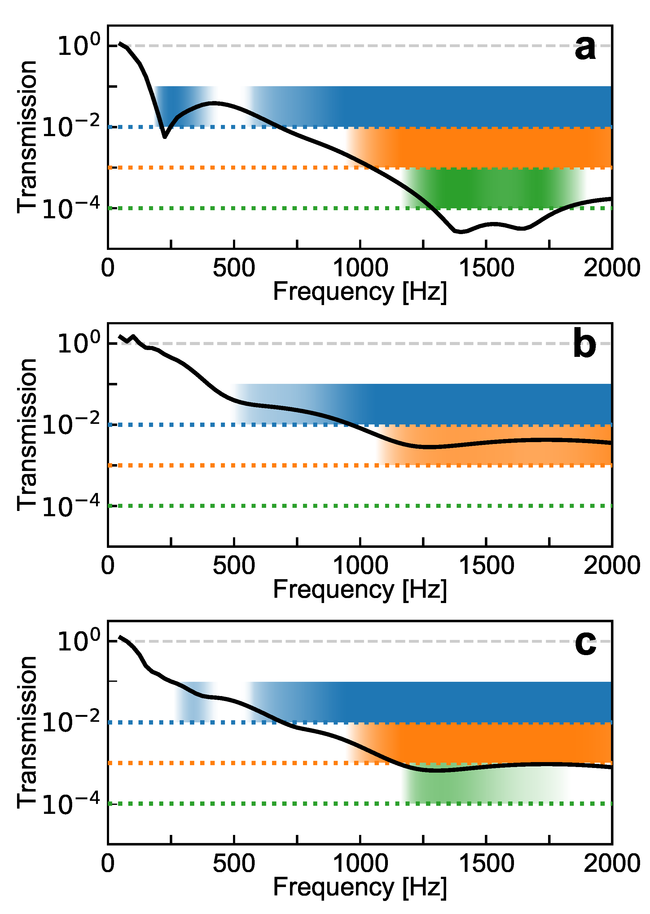
To further study how polarization hybridization affects the fuzzy band gaps, we compute the fuzzy band gaps for pure translation, pure rotation, and hybrid translation-rotation. For simplicity, we study polarizations with no frequency dependence, choosing the relative amplitudes of the experimental translation and rotation inputs at 1500 Hz (Figure 5c,d) as representative values for the amplitudes $L_y$ and ${\theta }_x$ of the states ${\mathbf{\psi }}_{TY}$ and ${\mathbf{\psi }}_{RX}$, respectively. In Figure 8, we plot the fuzzy band gaps for $N=5$ and $T_{thres}={10}^{-2},{10}^{-3},{10}^{-4}$. For pure translation (Figure 8a), the metastructure exhibits two fuzzy band gaps for $T_{thres}={10}^{-2}$, which collapse into a single fuzzy band gap for $T_{thres}={10}^{-3},{10}^{-4}$. The width of the fuzzy band gap is strongly affected by $T_{thres}$, with the fuzzy band gap width decreasing to about 750 Hz for $T_{thres}={10}^{-4}$. The shaded fuzzy band gaps capture all of the prominent features of the simulated transmission through an $N=5$ structure: the sharp, narrow trough in transmission near 250 Hz, the deep transmission trough between about 1350–1650 Hz, and the attenuation at high frequencies. For pure rotation (Figure 8b), there is only a single fuzzy band gap for $T_{thres}={10}^{-2},{10}^{-3}$. The metastructure is much less effective at attenuating rotationally polarized waves than translationally polarized waves, as evidenced by the lack of any fuzzy band gaps for $T_{thres}={10}^{-4}$ and by the increased transmission at high frequencies (−50 dB for rotation versus −80 dB for translation). The rotational fuzzy band gap for $T_{thres}={10}^{-3}$ is a “weak” fuzzy band gap; it does not reach fully saturated shading, indicating the transmission in the fuzzy band gap is near the threshold value. The dominance of the rotational mode is further illustrated by comparing the pure translational and pure rotational fuzzy band gaps (Figure 8a,b) with the hybrid fuzzy band gaps (Figure 8c). The hybrid fuzzy band gaps closely resemble the rotational fuzzy band gaps, with only a single fuzzy band gap at $T_{thres}={10}^{-2},{10}^{-3}$ and no fuzzy band gap at $T_{thres}={10}^{-4}$. The narrow low-frequency fuzzy band gap that existed for pure translation with $T_{thres}={10}^{-2}$ is obscured by the transmission of the rotational modes. However, the translational mode can be seen to cause a slight offset between the low-frequencies edges of the pure rotational and hybrid fuzzy band gaps, and also causes a 10 dB increase in the maximum attenuation achieved by the structure. The relative contribution of the translational and rotational modes naturally depends on the relative values of $L_y$ and ${\theta }_x$. For example, if $L_y$ is increased by a factor of three relative to the value chosen for Figure 8, the contribution of the translational modes becomes significant enough for a narrow low-frequency fuzzy band gap to appear in the hybrid-polarized mode.

5. Discussion

The proposed evanescence indicator provides a flexible and robust way to identify frequency ranges of strong wave attenuation in damped PCs which are termed “fuzzy” band gaps, including polarized fuzzy band gaps and hybrid-polarized fuzzy band gaps. In contrast to prior methods that heuristically identify regions of relatively greater or lesser evanescence in damped band structures, or rely on manual inspection and value judgments of mode shapes to classify polarizations, the proposed indicator quantitatively identifies fuzzy band gaps based on measurable physical quantities.

As a consequence of the generalized definition of fuzzy band gaps in damped PCs, fuzzy band gaps can not be defined unambiguously. In contrast to traditional band gaps which are unambiguously defined as any frequency where all wave modes are evanescent, the proposed method includes two arbitrary parameters (N and $T_{thres}$) that affect the fuzzy band gaps. These parameters can be based on physical arguments, so that fuzzy band gaps identified using this method can be related to experiments or simulations of finite structures. Alternatively, a single value of N and $T_{thres}$ can be selected to provide a consistent comparison between different geometries or polarizations, or fuzzy band gaps can be visualized for different combinations of N and $T_{thres}$ to illustrate how the choice of these parameters affects the computed fuzzy band gaps. In all cases, the chosen values of N and $T_{thres}$ should be reported.

To obtain the most accurate results, one must ensure that the computed dispersion relation is sufficiently complete, that is, that all relevant wavenumbers are computed by the eigenvalue search algorithm. In particular, FEM packages may utilize eigenvalue solvers that compute only a small fraction of the eigenvalues of the system. To accurately compute the evanescence indicator, it is important that all modes with small $|k_I|$ are computed by the eigenvalue solver, as they exhibit the slowest decay and therefore carry the most wave energy. Further analysis is needed to provide guidance on the minimum value of $|k_I|$ that should be included. One should also ensure that eigenvalues outside the first Brillouin zone, which may be returned by eigenvalue solvers, are not included in the computation of the evanescence indicator, as including them would result in double-counting the modes inside the first Brillouin zone.

Though the evanescence indicator was able to accurately identify the fuzzy band gaps when using the MPF method to compute the modal amplitudes, a puzzling result of this work was that the PBME method did not yield modal amplitudes which accurately captured the behavior of finite MAE metastructures. The reasons for this are not entirely clear. One possible explanation is that the normal modes of the finite structure do not resemble the propagated Bloch modes, because the Bloch modes are not compatible with the applied boundary condition of uniform longitudinal displacement. Further research is needed to understand if and how the PBME method can be applied to multiply-connected periodic media. Even still, the evanescence indicator accurately captures details of vibration transmission through finite MAE metastructures calculated through simulations and measured in vibration experiments.

There are a number of opportunities to extend and improve the current evanescence indicator. At present, the method is limited to structures with 1D periodicity. Generalizing this method to 2D and 3D periodicity would be of great value, but is more complicated as the flow of energy is not necessarily parallel to wave propagation direction. Thus, the wave transmission between the chosen input and output locations, and thus the value of the evanescence indicator, may depend more on the direction of the group velocity than the direction of the wavevector, and appropriate selection of the input and output locations takes on additional significance.

6. Conclusions

In this article, we developed a figure of merit called an “evanescence indicator” which gives a quantitative measure of wave decay in damped phononic crystals (PCs). We introduce a generalized definition of fuzzy band gaps as frequency ranges where the evanescence indicator falls below a threshold value, which we use to identify fuzzy band gaps in damped PCs. Using the 1D viscoelastic diatomic lattice as an example system, we show that the evanescence indicator predicts fuzzy band gaps that quantitatively agree with wave transmission through finite damped lattices. In particular, the evanescence indicator predicts fuzzy band gaps that coincide with the frequencies where finite transmission falls below the fuzzy band gap threshold. A novel result of the evanescence indicator is the “fuzziness” of fuzzy band gap edges, in which the fuzzy band gap edges occur as a gradual transition over a range of frequencies, in contrast to the discrete edge frequencies observed in undamped systems. We also apply the evanescence indicator to the magneto-active elastomer (MAE) metastructures introduced in [11], and demonstrate that the evanescence indicator accurately predicts fuzzy band gaps in PCs composed of real, highly damped materials. We verify the evanescence indicator using finite element method simulations and vibration experiments of finite MAE metastructures, and show that the evanescence indicator can identify fuzzy band gaps with respect to arbitrary wave polarizations, including hybrid wave polarizations which consist of two or more simultaneous polarizations. Our results show that the ability of the evanescence indicator to simultaneously consider multiple simultaneous wave polarizations (e.g., flexural and torsional) is significant, as each polarization makes a significant contribution to the fuzzy band gaps. This result emphasizes the importance of understanding and accounting for all relevant wave polarizations when studying polarized band gaps.

The evanescence indicator is particularly promising as a tool for understanding experimental results of physically realized PCs, due to its ability to (1) consider multiple simultaneous wave polarizations, (2) capture the effect of damping (which is present in all real materials), and (3) directly relate to measurable quantities (e.g., displacement) of physical systems. Conversely, the evanescence indicator could also be a useful design tool for developing real-world applications of PCs, as it requires only a single computation of the dispersion relation to predict fuzzy band gaps for finite phononic structures with arbitrary size and excitation polarization. By reducing the need to iteratively simulate finite PCs with different sizes and excitations, the evanescence indicator method could shorten the design time and accelerate the introduction of PCs into everyday life.

References

- Sigalas, M.M.; Economou, E.N. Elastic and acoustic wave band structure. J. Sound Vib. 1992, 158, 377–382. [Google Scholar] [CrossRef]
- Xu, Z.; Wu, F. Elastic band gaps of magnetorheological elastomer vibration isolators. J. Intell. Mater. Syst. Struct. 2015, 26, 858–864. [Google Scholar] [CrossRef]
- Wu, T.C.; Wu, T.T.; Hsu, J.C. Waveguiding and frequency selection of Lamb waves in a plate with a periodic stubbed surface. Phys. Rev. 2009, 79, 1–6. [Google Scholar] [CrossRef]
- Tol, S.; Degertekin, F.L.; Erturk, A. 3D-printed phononic crystal lens for elastic wave focusing and energy harvesting. Addit. Manuf. 2019, 29, 100780. [Google Scholar] [CrossRef]
- Frazier, M.J.; Hussein, M.I. Dissipation-triggered phenomena in periodic acoustic metamaterials. Health Monit. Struct. Biol. Syst. 2012 2012, 8348, 83481W. [Google Scholar] [CrossRef]
- Krattiger, D.; Khajehtourian, R.; Bacquet, C.L.; Hussein, M.I. Anisotropic dissipation in lattice metamaterials. AIP Adv. 2016, 6. [Google Scholar] [CrossRef]
- Liu, Z.; Zhang, X.; Mao, Y.; Zhu, Y.Y.; Yang, Z.; Chan, C.T.; Sheng, P. Locally resonant sonic materials. Science 2000, 289, 1734–1736. [Google Scholar] [CrossRef]
- Bertoldi, K.; Boyce, M.C. Mechanically triggered transformations of phononic band gaps in periodic elastomeric structures. Phys. Rev. B 2008, 77, 052105. [Google Scholar] [CrossRef] [Green Version]
- Bayat, A.; Gordaninejad, F. Band-Gap of a Soft Magnetorheological Phononic Crystal. J. Vib. Acoust. 2015, 137, 011011. [Google Scholar] [CrossRef]
- Xu, Z.; Wu, F.; Guo, Z. Shear-wave band gaps tuned in two-dimensional phononic crystals with magnetorheological material. Solid State Commun. 2013, 154, 43–45. [Google Scholar] [CrossRef]
- Pierce, C.D.; Willey, C.L.; Chen, V.W.; Hardin, J.O.; Berrigan, J.D.; Juhl, A.T.; Matlack, K.H. Adaptive elastic metastructures from magneto-active elastomers. Smart Mater. Struct. 2020, 29, 065004. [Google Scholar] [CrossRef]
- Moiseyenko, R.P.; Laude, V. Material loss influence on the complex band structure and group velocity in phononic crystals. Phys. Rev. B 2011, 83, 064301. [Google Scholar] [CrossRef] [Green Version]
- Hussein, M.I. Theory of damped Bloch waves in elastic media. Phys. Rev. B 2009, 80, 212301. [Google Scholar] [CrossRef]
- Hussein, M.I.; Frazier, M.J. Band structure of phononic crystals with general damping. J. Appl. Phys. 2010, 108. [Google Scholar] [CrossRef]
- Frazier, M.J.; Hussein, M.I. Generalized Bloch’s theorem for viscous metamaterials: Dispersion and effective properties based on frequecies and wavenumbers that are simultaneously complex. Comptes Rendus Phys. 2016, 17, 565–577. [Google Scholar] [CrossRef]
- Hussein, M.I. Reduced bloch mode expansion for periodic media band structure calculations. Proc. R. Soc. A 2009, 465, 2825–2848. [Google Scholar] [CrossRef] [Green Version]
- Hussein, M.I.; Frazier, M.J. Metadamping: An emergent phenomenon in dissipative metamaterials. J. Sound Vib. 2013, 332, 4767–4774. [Google Scholar] [CrossRef] [Green Version]
- Bacquet, C.L.; Al Ba’Ba’a, H.; Frazier, M.J.; Nouh, M.; Hussein, M.I. Metadamping: Dissipation Emergence in Elastic Metamaterials. Adv. Appl. Mech. 2018, 51, 115–164. [Google Scholar] [CrossRef]
- Aladwani, A.; Nouh, M. Mechanics of metadamping in flexural dissipative metamaterials: Analysis and design in frequency and time domains. Int. J. Mech. Sci. 2020, 173, 105459. [Google Scholar] [CrossRef]
- Frazier, M.J.; Hussein, M.I. Viscous-to-viscoelastic transition in phononic crystal and metamaterial band structures. J. Acoust. Soc. Am. 2015, 138, 3169–3180. [Google Scholar] [CrossRef] [Green Version]
- Wang, T.T.; Laude, V.; Kadic, M.; Wang, Y.F.; Wang, Y.S. Complex-Eigenfrequency Band Structure of Viscoelastic Phononic Crystals. Appl. Sci. 2019, 9, 2825. [Google Scholar] [CrossRef] [Green Version]
- Andreassen, E.; Jensen, J.S. Analysis of phononic bandgap structures with dissipation. J. Vib. Acoust. Trans. 2013, 135, 041015. [Google Scholar] [CrossRef]
- Chen, Y.; Guo, D.; Li, Y.F.; Li, G.; Huang, X. Maximizing wave attenuation in viscoelastic phononic crystals by topology optimization. Ultrasonics 2019, 94, 419–429. [Google Scholar] [CrossRef] [PubMed]
- Collet, M.; Ouisse, M.; Ruzzene, M.; Ichchou, M.N. Floquet-Bloch decomposition for the computation of dispersion of two-dimensional periodic, damped mechanical systems. Int. J. Solids Struct. 2011, 48, 2837–2848. [Google Scholar] [CrossRef] [Green Version]
- Krushynska, A.O.; Kouznetsova, V.G.; Geers, M.G.D. Visco-elastic effects on wave dispersion in three-phase acoustic metamaterials. J. Mech. Phys. Solids 2016, 96, 29–47. [Google Scholar] [CrossRef] [Green Version]
- Laude, V.; Achaoui, Y.; Benchabane, S.; Khelif, A. Evanescent Bloch waves and the complex band structure of phononic crystals. Phys. Rev. B 2009, 80, 1–4. [Google Scholar] [CrossRef] [Green Version]
- Matlack, K.H.; Bauhofer, A.; Krödel, S.; Palermo, A.; Daraio, C. Composite 3D-printed metastructures for low-frequency and broadband vibration absorption. Proc. Natl. Acad. Sci. USA 2016, 113, 8386–8390. [Google Scholar] [CrossRef] [Green Version]
- Arretche, I.; Matlack, K.H. On the interrelationship between static and vibration mitigation properties of architected metastructures. Front. Mater. 2018, 5, 68. [Google Scholar] [CrossRef]
- Arretche, I.; Matlack, K.H. Experimental testing of vibration mitigation in 3D printed architected metastructures. J. Appl. Mech. 2019, 86, 111008. [Google Scholar] [CrossRef]
- Sen Gupta, G. Natural flexural waves and the normal modes of periodically-supported beams and plates. J. Sound Vib. 1970, 13, 89–101. [Google Scholar] [CrossRef]
- Faulkner, M.G.; Hong, D.P. Free vibrations of a mono-coupled periodic system. J. Sound Vib. 1985, 99, 29–42. [Google Scholar] [CrossRef]
- Hussein, M.I.; Hulbert, G.M.; Scott, R.A. Dispersive elastodynamics of 1D banded materials and structures: Analysis. J. Sound Vib. 2006, 289, 779–806. [Google Scholar] [CrossRef] [Green Version]
- Al Ba’ba’a, H.; Nouh, M.; Singh, T. Pole distribution in finite phononic crystals: Understanding Bragg-effects through closed-form system dynamics. J. Acoust. Soc. Am. 2017, 142, 1399–1412. [Google Scholar] [CrossRef] [PubMed]
- Al Ba’Ba’a, H.; Nouh, M. An investigation of vibrational power flow in one-dimensional dissipative phononic structures. J. Vib. Acoust. 2017, 139, 021003. [Google Scholar] [CrossRef]
- Inman, D.J. Engineering Vibration, 4th ed.; Pearson Education Limited: Essex, UK, 2014. [Google Scholar]
- Wijker, J. Mechanical Vibrations in Spacecraft Design, 1st ed.; Springer: Berlin, Germany, 2004. [Google Scholar] [CrossRef]
- Brillouin, L. Wave Propagation in Periodic Structures, 2nd ed.; Dover Publications, Inc.: New York, NY, USA, 1953; p. 255. [Google Scholar]
- Borland, D.; Taylor, R.M., II. Rainbow color map (still) considered harmful. IEEE Comput. Graph. Appl. 2007, 27, 14–17. [Google Scholar] [CrossRef]
- Rigbi, Z.; Jilkén, L. The response of an elastomer filled with soft ferrite to mechanical and magnetic influences. J. Magn. Magn. Mater. 1983, 37, 267–276. [Google Scholar] [CrossRef]
- Shamonin, M.; Kramarenko, E.Y. Highly Responsive Magnetoactive Elastomers. In Novel Magnetic Nanostructures, 1st ed.; Domracheva, N., Caporali, M., Rentschler, E., Eds.; Elsevier Inc.: Amsterdam, The Netherlands, 2018. [Google Scholar] [CrossRef]
Figure 1.
Schematic of a 1D diatomic lattice. The pth unit cell is shown, with lattice spacing , masses and , viscoelastic springs , and subject to forces and on the left and right boundaries. , , and are the displacements of the left and right boundaries and the internal dof, respectively.
Figure 2.
Effect of threshold amplitude and loss factor on the fuzzy band gaps of a 1D viscoelastic diatomic lattice: (a) , (b) , and (c) . Solid black lines: evanescence indicator; dashed black lines: transmission through finite structure computed using full set of DOFs; dotted lines: three selected values of the threshold transmission : (blue), (orange), and (green). Shaded bars indicate fuzzy band gaps for the value of the corresponding color.
Figure 3.
Effect of threshold amplitude and the size of the structure of reference N on the fuzzy band gaps of a 1D viscoelastic diatomic lattice with : (a) , (b) , and (c) . Solid black lines: evanescence indicator; dashed black lines: transmission through finite structure computed using full set of DOFs; dotted lines: three selected values of the threshold transmission : (blue), (orange), and (green). Shaded bars indicate fuzzy band gaps for the value of the corresponding color.
Figure 4.
Band structure for the 1D viscoelastic diatomic lattice: (a) and (b) . Fuzzy band gaps computed with , are shown for (c) , (d) , and (e) .
Figure 5.
Experimental determination of wave transmission in a magneto-active elastomer (MAE) metastructure for transverse excitations. (a) Side view of experimental setup. Metastructure (a1) is excited by an electrodynamic shaker (a2). A linear guide (a3) confines displacement to the y-direction. (b) Front view of metastructure indicating nine input measurement locations (b2) on the acrylic block and 11 output measurement locations (b1) on the free end of the metastructure. (c) Frequency spectrum of the input velocities. Divergence of the input velocities above 1.25 kHz indicates the emergence of rigid body rotation. (d) Input mode shape at 1.5 kHz: black—experimental velocity; blue—rigid body translation; orange—rigid body rotation; white markers and dashed line—superposition of rigid body translation and rotation.
Figure 6.
MAE metastructure results for longitudinally-polarized waves. (a) Damped dispersion relation, with the hue of each point determined by for the corresponding Bloch mode shape, and the transparency determined by , as shown in the colorbar above the plot. “Frustrated” modes have at . The “equal evanescence point” (EEP) between the resonator and first frustrated mode is indicated by the arrow. (b) Undamped dispersion relation, with the hue of each point determined by as shown in the colorbar above the plot. The longitudinal band gap is shaded in gray. (c) Transmission through an finite structure: blue line—FEM, orange line—experimental. In panels (a,b), modes with a strong longitudinal polarization are colored yellow or green while other modes are colored blue or purple. In panels (a,c), fuzzy band gaps are computed using the evanescence indicator with and , and the dashed blue line in panel (c) indicates .
Figure 7.
MAE metastructure results for transverse (y)-polarized waves. (a) Damped dispersion relation, with the hue of each point determined by the maximum value of and for the corresponding Bloch mode shape, and the transparency determined by , as shown in the colorbar above the plot. (b) Undamped dispersion relation, with the hue of each point determined by as shown in the colorbar above the plot. The transverse-polarized band gaps are shaded in gray. (c) Transmission through an finite structure: blue line—FEM, orange line—experimental. In panels (a,b), modes with a strong transverse polarization are colored yellow or green while other modes are colored blue or purple. In panels (a,c), fuzzy band gaps are computed using the evanescence indicator with and , and the dashed blue line in panel (c) indicates .
Figure 8.
Polarized fuzzy band gaps in the MAE metastructure: (a) translational (y) only, (b) rotational (x-axis) only, and (c) simultaneous translation (y) and rotation (x-axis). Dotted lines indicate threshold tranmission (blue), (orange), (green), and solid black lines indicate FEM-simulated transmission.
Publisher’s Note: MDPI stays neutral with regard to jurisdictional claims in published maps and institutional affiliations. |
© 2021 by the authors. Licensee MDPI, Basel, Switzerland. This article is an open access article distributed under the terms and conditions of the Creative Commons Attribution (CC BY) license (http://creativecommons.org/licenses/by/4.0/).
Share and Cite
MDPI and ACS Style
Pierce, C.D.; Matlack, K.H. “Fuzzy Band Gaps”: A Physically Motivated Indicator of Bloch Wave Evanescence in Phononic Systems. Crystals 2021, 11, 66. https://0-doi-org.brum.beds.ac.uk/10.3390/cryst11010066
AMA Style
Pierce CD, Matlack KH. “Fuzzy Band Gaps”: A Physically Motivated Indicator of Bloch Wave Evanescence in Phononic Systems. Crystals. 2021; 11(1):66. https://0-doi-org.brum.beds.ac.uk/10.3390/cryst11010066
Chicago/Turabian StylePierce, Connor D., and Kathryn H. Matlack. 2021. "“Fuzzy Band Gaps”: A Physically Motivated Indicator of Bloch Wave Evanescence in Phononic Systems" Crystals 11, no. 1: 66. https://0-doi-org.brum.beds.ac.uk/10.3390/cryst11010066
Note that from the first issue of 2016, this journal uses article numbers instead of page numbers. See further details here.