Boundary Conditions for Simulations of Fluid Flow and Temperature Field during Ammonothermal Crystal Growth—A Machine-Learning Assisted Study of Autoclave Wall Temperature Distribution

Abstract

Thermal boundary conditions for numerical simulations of ammonothermal GaN crystal growth are investigated. A global heat transfer model that includes the furnace and its surroundings is presented, in which fluid flow and thermal field are treated as conjugate in order to fully account for convective heat transfer. The effects of laminar and turbulent flow are analyzed, as well as those of typically simultaneously present solids inside the autoclave (nutrient, baffle, and multiple seeds). This model uses heater powers as a boundary condition. Machine learning is applied to efficiently determine the power boundary conditions needed to obtain set temperatures at specified locations. Typical thermal losses are analyzed regarding their effects on the temperature distribution inside the autoclave and within the autoclave walls. This is of relevance because autoclave wall temperatures are a convenient choice for setting boundary conditions for simulations of reduced domain size. Based on the determined outer wall temperature distribution, a simplified model containing only the autoclave is also presented. The results are compared to those observed using heater-long fixed temperatures as boundary condition. Significant deviations are found especially in the upper zone of the autoclave due to the important role of heat losses through the autoclave head.

1. Introduction

Solvothermal crystallization processes are widely used for growth of bulk crystals as well as particle syntheses. Solvothermal syntheses typically utilize fluids near or sometimes even far above their critical parameters in order to make use of enhanced solvent properties, such as a combination of high diffusivity and low viscosity that facilitates mass transport [1].

A variety of solvents are used, with water being the most abundant example. However, nonaqueous solvents are increasingly being researched. Specifically, supercritical ammonia has emerged as the solvent of choice for the synthesis of various nitride materials [2], with the method termed ammonothermal in analogy to the term hydrothermal for syntheses that use supercritical water as a solvent. While nitrides represent a group of materials of which many materials are yet to be discovered experimentally [3], the most intensively researched nitride material grown by the ammonothermal method is bulk GaN.

Due to its high electric field strength and high electron mobility, GaN is an outstanding material for power electronic devices [4,5] and enables new applications that cannot be realized with conventional Si-based power electronics [4]. In particular, GaN devices allow for very low specific on-resistance, hence, significant improvements in the energy-efficiency of power conversion devices can be expected from GaN [4]. This is of increasing importance due to recent, sustainability-driven developments, such as the trend towards mass-adoption of electric vehicles and the increasing use of renewable energy sources [4]. For high power applications, it is desirable to use vertical device architectures (i.e., with the current flow through the substrate) because such devices can handle much higher current densities and operate at higher voltages than lateral devices [6]. Vertical GaN-on-GaN devices require GaN substrates with low dislocation density [6]. For the above reasons, making high-quality bulk GaN available at a competitive price will have a large impact on power electronics for a sustainable society.

The ammonothermal method is an exceptionally promising and well-scalable method for growth of high-quality GaN and has already made impressive progress. Single crystals of nearly 4 inch size achieved by an ammonoacidic method has recently been demonstrated [7]. Moreover, scalability towards growth of many crystals within one run has been shown for 2 inch size crystals using an ammonobasic method [8]. Besides their potential for mass production, ammonothermal methods yield access to single crystals of exceptionally high structural quality, for instance in terms of dislocation densities and radius of curvature [9], which is particularly important for applications in vertical power electronic devices. Methods for controlling impurity concentrations based on corrosion protection [10], in-autoclave synthesis of mineralizers [11] or the use of getters [12] have also been developed.

Despite all these achievements, scale-up still requires a large amount of trial-and-error based optimization of growth conditions. Numerical simulations are one way to guide scale-up as well as to advance the understanding of underlying processes. Several groups have studied ammonothermal growth by numerical simulations [13,14,15,16]; however, there are several factors of uncertainty regarding the accuracy of such simulations. Validation data are scarce due to the difficulty of experimental access at process conditions around 400 to 650 °C and 100 to 300 MPa. This work aims to shine light at one such factor of uncertainty, namely the temperature distribution in the walls of an ammonothermal autoclave. In most of the literature, outer wall temperatures are assumed to be constant within the length of one heater (or similar wall sections) and this assumption is used to define boundary conditions [13,16,17]. It is worth noting that for another solvothermal method, the hydrothermal growth of quartz, the temperature distribution at the inner autoclave wall has been reported to be far from uniform within the actively heated sections of the wall [18]. There is one previous study of an ammonothermal setup including the furnace and using heater power as a boundary condition [14]. However, this study neglected convective contributions to heat transfer in the first (2D) model that was used to determine wall temperature distribution [14], so the question arises whether the influence of convection on wall temperatures is negligible. Erlekampf et al. [14] do present validation data; however, the investigated temperature configuration must be expected to minimize the influence of convective heat transfer, given that for some reason the top of the autoclave is held at a higher temperature than the bottom. Note that regardless of the mineralizer used, the opposite temperature distribution is commonly used in the growth phase of bulk crystal growth experiments in order to favor convective mass transport (see for instance [19] for an overview of the method and typical configurations). In spite of the buoyancy-suppressing configuration, Erlekampf et al. observe a deviation between simulation and validation data of about 15 K near the bottom of the autoclave, which they ascribe to neglecting the influence of convective heat transfer in the calculation that included the furnace and that was used to determine thermal boundary conditions to the 3D flow simulation. The nearly constant temperature in radial direction in both their validation and simulation data [14] also points towards a low contribution of buoyancy which could be just due to the inverted temperature zone settings. In summary, further investigation is needed for the growth phase, and it may be necessary to couple heat transfer and flow simulations even for studying global heat transfer in the entire growth furnace. In addition, Erlekampf et al. [14] (as the only authors who have studied the global thermal field in an ammonothermal growth furnace) have presented information neither on the global thermal field inside the furnace nor on the temperature distribution within the autoclave walls. The present study also fills this gap.

While acknowledging that both fixed, section-wise constant temperature boundary conditions and the use of separate models for wall temperature distribution and fluid flow (i.e., the two approaches seen in literature) greatly simplify calculations, this work aims to clarify whether those simplifications can be expected to yield sufficiently accurate results. Note that buoyancy-driven convection can be significantly affected also by deviations from perfectly adiabatic or perfectly conducting, not actively heated enclosure walls [20]. Such effects have just recently been investigated for water in cuboid enclosures by Ferialdi et al. who employed both numerical methods and experimental validation by flow visualization, indicating that such effects remain an active field even of fundamental research [20]. As Ferialdi et al. point out, the effective heat exchange taking place through not actively heated walls may very well be of practical relevance, in particular if meaningful comparison of numerical and experimental results is targeted [20].

2. Materials and Methods

Including the furnace in simulation poses the challenge that the heat sources are spatially separated from the controlled temperatures. In the case of ammonothermal autoclaves, precise temperature control is very important and therefore, thermocouples for control of the furnace are typically placed directly at the outer autoclave wall, with special measures taken to ensure proper thermal contact [10]. Initial simulations conducted in this study have shown that neither the temperature distribution in the autoclave walls nor in the heating elements of the furnace are homogeneous. Therefore, it is thought to be most accurate to use the power that is supplied to the heating elements as boundary conditions.

2.1. Simulations of Temperature Distribution and Fluid Flow

Numerical models of an ammonothermal setup were set up using the commercial software Phoenics (Concentration, Heat and Momentum Limited (CHAM)), which uses the SIMPLEST (SIMPLE ShorTened) algorithm. Simulations were conducted effectively in 2D. Although there is a literature work suggesting that 3D simulations may be necessary for accurately modeling heat and mass transfer in ammonothermal systems [14], 2D simulations were deemed appropriate for the purpose of this study. Since the focus of this study is on boundary conditions at the outer autoclave wall and their effect on temperature and flow field inside the autoclave, short-term fluctuations due to three-dimensional flow are not expected to have a major effect on the results of this study. Similarly, also the effects of non-axisymmetric solids, namely the seeds, are not expected to be negligible for a detailed study of internal fluid flow. However, the global effects of their lack of symmetry are thought to be rather small. In particular, neither short-term fluctuations in fluid flow nor the cuboid shape of the seeds are expected to affect the main goal of this study, which is to identify suitable types of boundary conditions at the outer autoclave wall or at the active part of the heaters. On the other hand, a large amount of computational time is saved by using 2D simulations, given the large domain size that is necessary for studying the heat transfer in the furnace and its surroundings.

Note that for the finite-volume numerical solution method employed in Phoenics CFD software, a nonzero volume is required also for a 2D simulation. Therefore, a nonzero third dimension is required, although the choice of this dimension (in which only one mesh cell exists) is of no fundamental significance. It is, however, important to note that absolute quantities related to the volume or surface area of objects depend on this third dimension. For this reason, heater powers needed to maintain certain temperatures in the here presented simulations cannot directly be compared to experimentally used heater powers. The third dimension was set to 1 mm; therefore, the simulation domain represents a 1 mm thick slice through half of the experimental setup (approximating the experimental setup as axially symmetric). Accordingly, the powers required to keep the simulation domain at a given temperature are small compared to the heater output required to maintain the same temperatures in the complete volume of an experimental setup.

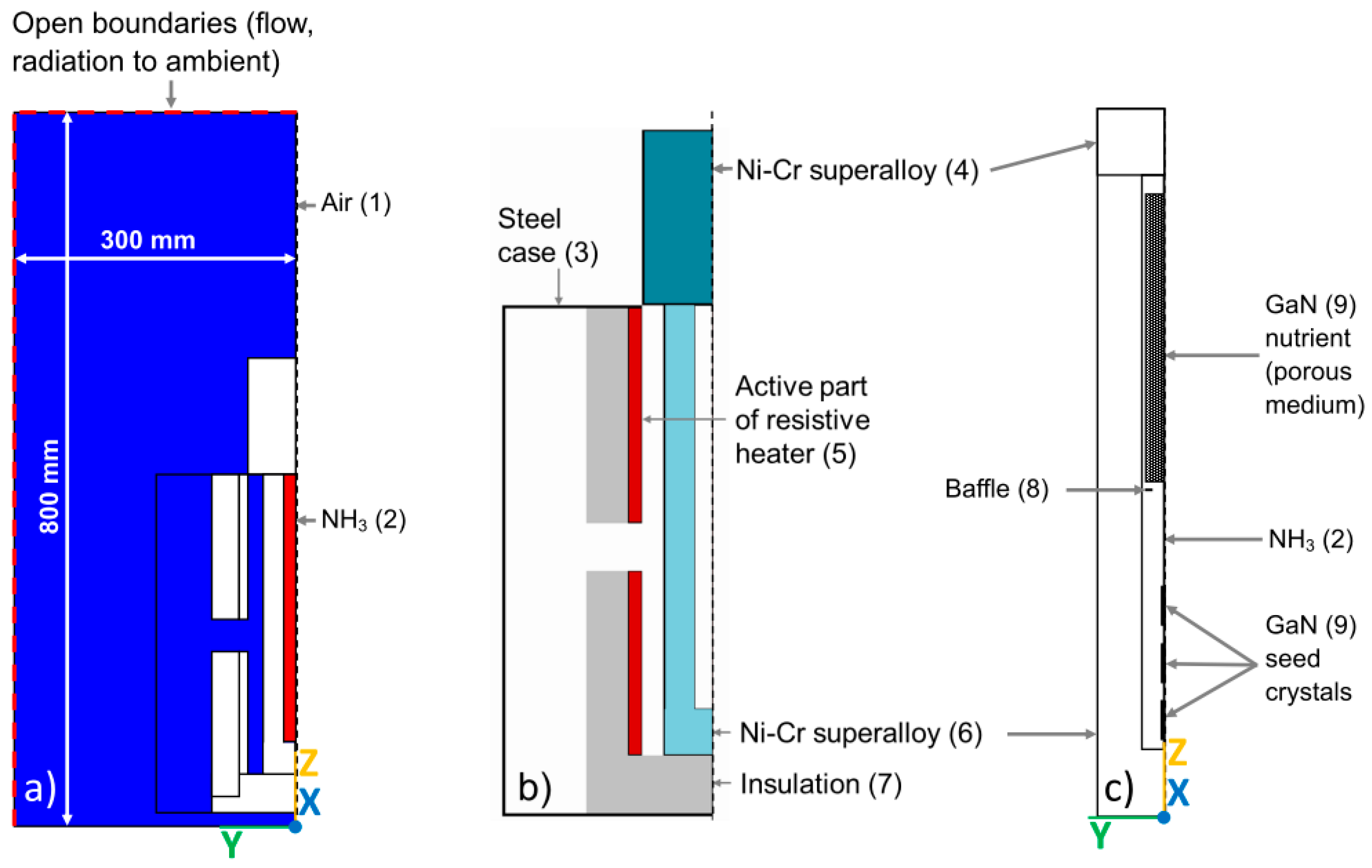
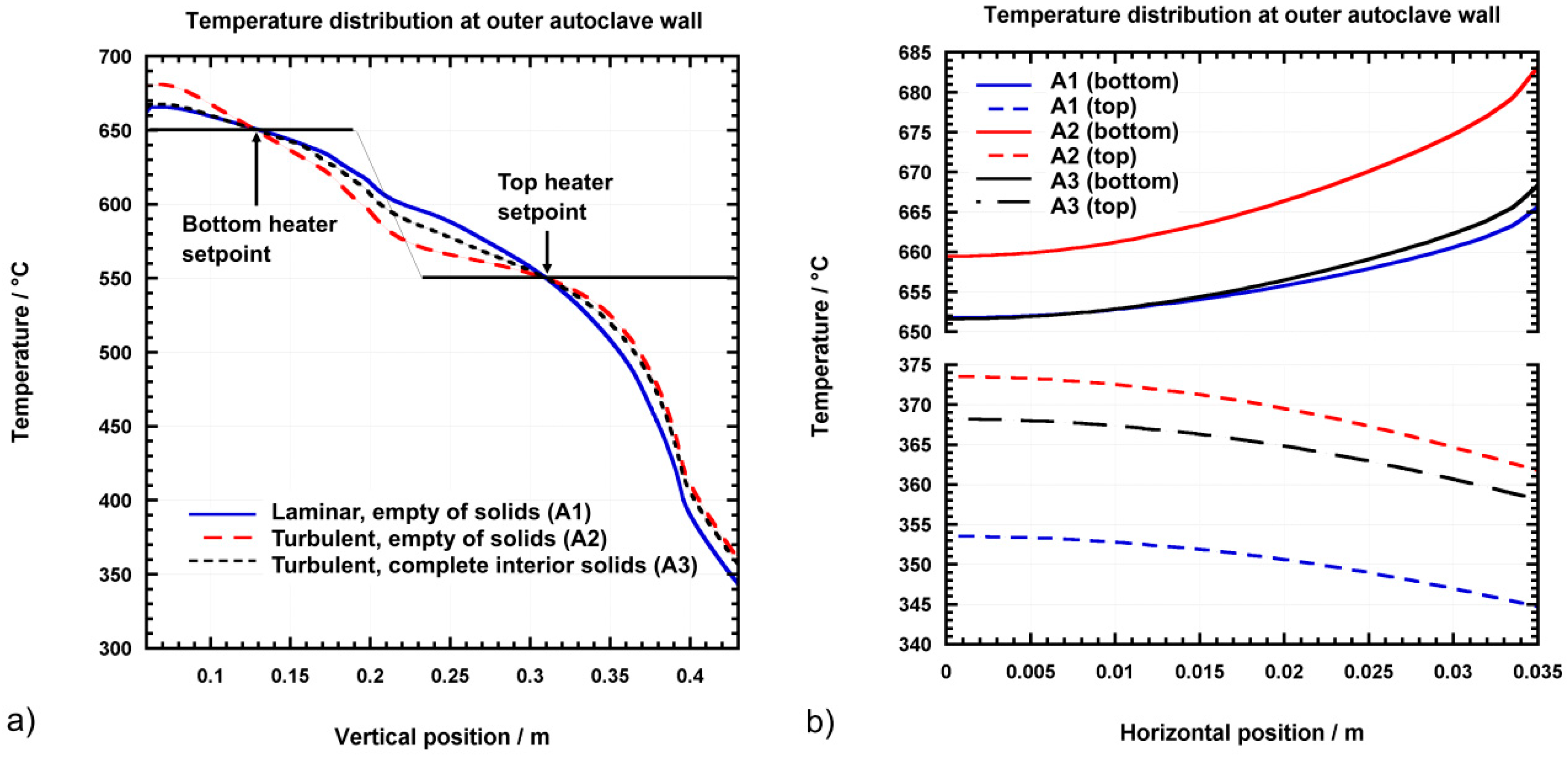
The geometry was based on ammonoacidic literature assuming retrograde solubility [21,22] for the placement of seeds and nutrient. Three types of simulation cases were used in this study. They will be termed A, B, and C. Cases of type A include the entire setup including the furnace and its surrounding. The geometry of type A cases is depicted in Figure 1a,b. The locations of control temperature measurement (corresponding to thermocouple locations in experimental work) were 310 mm and 130 mm above the bottom domain boundary of the type A cases. The lateral position of the control temperature measurement locations was 32 mm, which is 3 mm inwards from the surface of the outer autoclave wall and ensures evaluation of stable autoclave wall temperatures that are not significantly affected by short-term fluctuations in convective flow of the surrounding air inside the furnace. Fluid flow was considered both inside the autoclave and in air-filled spaces of the furnace, i.e., in both the blue and red regions in Figure 1a. Dimensions and materials of the autoclave and furnace are given in Figure 1b. Note that these dimensions also apply to cases of types B and C, of which the simulation domain and geometry is shown in Figure 1c. 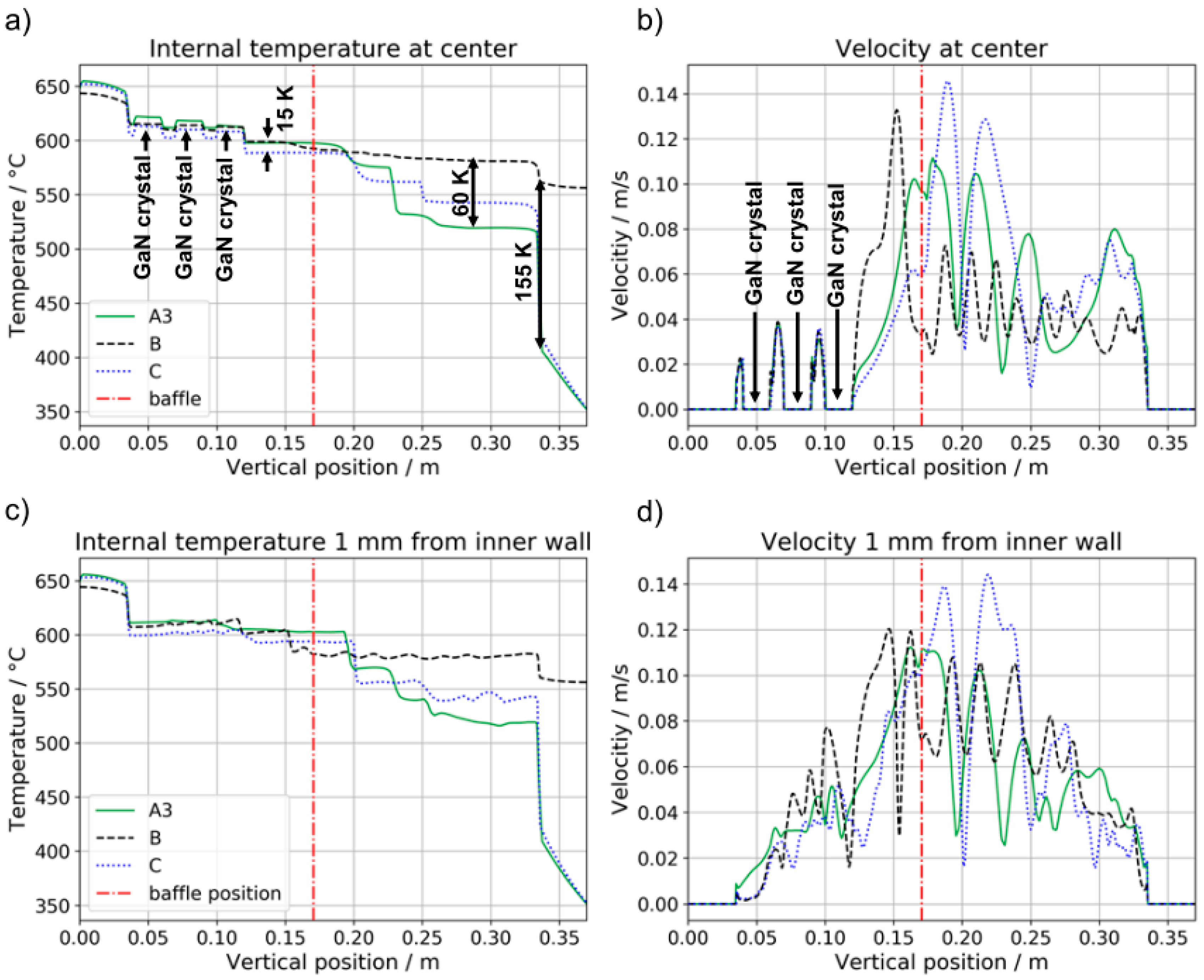Vice versa, the materials and dimensions of the solids inside the autoclave that are indicated in Figure 1c also apply to type A cases if interior solids were present therein. The vertical length of each seed was 20 mm, and the lateral width was 3 mm (of which 1.5 mm were inside the simulation domain). The center of the seeds was positioned 75 mm, 45 mm, and 15 mm above the bottom inner wall, respectively. The ring-shaped baffle had an inner radius of 6.6 mm and an outer radius of 10 mm, resulting in and open space ratio (OSR) of 30.25%. The thickness of the baffle was 1 mm. The center of the baffle was located 135 mm above the bottom inner wall. The radius of the nutrient was 10 mm, and the height of the nutrient was 150 mm. The center of the nutrient was placed 215 mm above the bottom inner wall.

In order to investigate how different fixed-temperature boundary conditions at the outer autoclave wall can yield similarly accurate results at lower computational cost, a simplified model containing only the autoclave was set up. Depending on the fixed-temperature boundary condition used, this simplified model will be termed type B and C, respectively. Type B represents cases with heater-long fixed temperatures and otherwise adiabatic walls whereas type C uses the temperature distribution determined for the outer autoclave wall by an analogous type A simulation. (A complete list of conducted simulation cases and the motivation for the choice of conditions will be given in Table 4 and the corresponding text section.)

An overview of the materials used is given in

Table 1. Overview of materials used in simulation of temperature distribution and fluid flow.

Material	Description
Air (1)	At 20 °C, 1 atm, treated as incompressible
NH3 (2)	At 426.6 °C, 100 MPa, treated as incompressible
Steel (3)	At 27 °C, C = 1%
Ni-Cr superalloy (4)	At 600 °C
Active part of resistive heater (5)	At 600 °C
Ni-Cr superalloy (6)	At 538 °C
Insulation (7)
Baffle (8)
GaN (bulk) (9)	Wurtzite GaN

. The numbers in brackets are used in subsequent tables as well as Figure 1 to refer to the materials.

The materials properties used are given in

Table 2. Material properties of fluids in simulation of temperature distribution and fluid flow. Data for air (at ambient temperature) were taken from Phoenics inbuilt database, data for supercritical ammonia at 426.9 °C (the upper end of the temperature range for which data are available) were obtained from NIST database [24].

Gas/Fluid	ρ/(kg/m3)	ν/(m2/s)	cp/(J/(kg∙K))	k/(W/(m∙K)	α/(1/K)	β/(m2/N)
Air (1)	1.189	1.544 × 10−5	1005.0	0.02580	3.410 × 10−3	0.0
NH3,sc (2)	233.950	1.570 × 10−7	4216.5	0.16224	2.631 × 10−3	0.0

for fluids and

Table 3. Material properties of solids in simulation of temperature distribution and fluid flow.

Solid	ρ/(kg/m3)	cp/(J/(kg∙K))	k/(W/(m∙K)	(1/E)/(m2/N)	ε/(1)
Steel (3)	7800.0	473.00	43.00	0.50 × 10−11	0.2
Ni-Cr superalloy (4)	8260.0	533.00	20.60	6.00 × 10−6	0.8
Active part of resistive heater (5)	7150.0	750.00	20.00	5.88 × 10−6	1.0
Ni-Cr superalloy (6)	8249.0	452.00	18.90	5.30 × 10−6	0.8
Insulation (7)	12.0	840.00	0.04	1.00 × 10−9	0.2
Baffle (8)	10,220.0	251.00	138.00	3.03 × 10−6	1.0
GaN (bulk) (9)	6150.0	518.41	100.13	3.39 × 10−6	1.0

for solids, respectively. To account for the temperature dependency of density as a driving force for buoyancy, Boussinesq approximation was used to model natural convection. This implies assuming that density variations are negligibly small everywhere except in the gravitational term, and that density is a linear function of temperature T1. In this case, density variations do not appear explicitly in the momentum equations. Density variations are thus described as a function of temperature T1 as follows (Equation (1)) [23]:

$$\rho -{\rho }_{ref}=-{\rho }_{ref}{\alpha }_v\left(T_1 - T_{ref}\right).$$

(1)

The reference density ${\rho }_{ref}$ is a constant density chosen as the density of air at ambient conditions. ${\alpha }_v$ represents the volumetric thermal expansion coefficient. Multiplying the term $\rho -{\rho }_{ref}$ with gravity g yields the buoyancy force.

The energy equation was formulated in terms of temperature (Equation (2)) [23]:

$$\begin{array}{c}{M}_{t-1}\left(c_{p,eff} T_{t-1}-c_{p,eff} T_t\right)/dt\\ +m_{+}\left(c_{p,eff,+}{T}_{t,+}-c_{p,eff}{T}_t\right)+m_{-}\left(c_{p,eff,-}{T}_{t,-}-c_{p,eff}{T}_t\right)\\ -\left(A_{+}{k}_{+}/d{X}_{+}\right)\left(T_t-T_{+}\right)-\left(A_{-}{k}_{-}/d{X}_{-}\right)\left(T_t-T_{-}\right)=0.\end{array}$$

(2)

Therein, the subscripts (+/−) refer to the neighbor cells in positive/negative direction. Subscript t refers to the current time-step whereas subscript t−1 refers to the previous time-step. Thus, for instance, $M_{t-1}$ is the mass of fluid in the cell described by equation 2, at the previous time-step. The mass in-flow rate is denoted as m. A represents the cell-face area and dX the distance between cell centers. The thermal conductivity is denoted as k. Conservation of mass is implied. The energy source term $c_{p,eff}$ is an effective specific heat capacity and defined as $c_{p,eff} = \left(H - H_{abs}\right)/T_{abs}$. Therein, H refers to the enthalpy, $H_{abs}$ is the enthalpy of the material at absolute zero, and $T_{abs}$ is the temperature on an absolute scale (i.e., in Kelvin).

Radiative heat transfer was implemented using Immersol model [25] because a significant contribution of radiation to the heat transfer from heaters to autoclave is expectable at growth temperatures. Immersol model uses the grey-medium approximation (i.e., neglects wavelength dependence). It is valid independently of the mean free path of radiation, i.e., for optically-thin and optically-thick gaps filled with transparent medium but also in-between those limits [23].

The radiosity J_e, i.e., the sum of all radiation fluxes traversing the volume (regardless of direction and wavelength) is defined by Equation (3):

$$J_e=\sigma T_3^4.$$

(3)

In Equation (2), σ is the Stefan–Boltzmann constant and T₃ is the radiosity temperature in Kelvin, which is a separate variable in Phoenics. At the boundaries of transparent medium and solids, as well as within solids, the radiosity temperature is equal to the first phase temperature T₁. The radiant flux at such boundaries, however, depends not only on the gradient of T₃ in the medium near the wall but also on the emissivity of the wall. The differential equation for T₃ is as follows (Equation (4)):

$$\nabla \left({\lambda }_3\nabla T_3\right) + {\dot{Q}}_{T3}=0.$$

(4)

Therein, λ₃ represents the thermal conductivity pertaining to the radiosity temperature T₃ described by Equation (5):

$${\lambda }_3=4\sigma T_3^3/\left\{0.75\left({\epsilon }_1^{\prime }+s_1^{\prime }\right)+1/W_{gap}\right\}.$$

(5)

Therein, ${\epsilon }_1^{\prime }$ is the emissivity per unit length and $s_1^{\prime }$ is the scattering coefficient per unit length, both referring to the phase in the space that is transparent to radiation. W_gap represents the gap between nearby solid walls. The source term ${\dot{Q}}_{T3}$ is related to the first phase temperature T₁ and the radiosity temperature T₃ by Equation (6):

$${\dot{Q}}_{T3}=-4{\epsilon }_1^{\prime }\sigma \left(T_3^4-T_1^4\right).$$

(6)

An in-depth description and rationalization of Immersol model can be found in [25].

Thermal losses were implemented through heat conduction, through natural convection and through radiation to the ambient. Air exchange was allowed at the top and side walls of the domain (domain walls at Y = + 300 mm and Z = + 800 mm in Figure 1a). Only natural convection was considered. However, note that thermal losses to the air surrounding the furnace would be higher if forced convection was considered in addition (this may be relevant in practice in some laboratories if there are high air turnovers, for example as a result of lab safety measures).

The fluid was treated as a clear fluid. Note, however, that transparency changes under ammonothermal process conditions have been reported for visible light for the GaN-NH₄Cl-NH₃-system [26] and that it is unknown whether the fluid remains clear to infrared radiation under process conditions.

Both laminar and turbulent flow were considered, as it seems not fully clarified what to expect inside the autoclave. For estimating dimensionless numbers, a flow speed maximum of 0.2 m/s as reported by Erlekampf et al. [14] was considered. Furthermore, one tenth of the maximum flow speed was also considered to account for regions of slower flow as well as uncertainty due to a lack of experimental data. Flow velocities in the order of 0.01 m/s occur in simulation results in literature (e.g., Chen et al. up to 0.06 m/s in the center gap of the baffle [27]). The definition by Lin and Akins is applied for determining the characteristic length for the calculation of dimensionless numbers, as they have proposed an approach specifically geared towards natural convection in enclosures [28]. For the considered fluid density of 233.95 kg/m³ and using linear extrapolation of NIST [24] data on viscosity to 550 °C (i.e., a dynamic viscosity of about 4.01 × 10⁻⁵ Pa∙s), the Reynolds number R is about 2.02 × 10³ for 0.02 m/s to 2.02 × 10⁴ for 0.2 m/s. Therefore, a transition from laminar to turbulent flow is expected to occur depending on the location inside the cavity. Prantl and Rayleigh numbers are about 1.04 and 2.51 × 10⁹, respectively, which strongly suggests turbulent flow (for the given Prantl number, a transition to turbulent flow can be expected at Rayleigh numbers around 2.5 × 10⁴ [29]). However, there are doubts as to how precisely extrapolated viscosity of pure ammonia matches the viscosity of the actual, solute-containing fluid [30]. A higher viscosity, as suspected based on in-situ x-ray monitoring of the diffusion of Ga-containing solutes [30], could push the Reynolds and Rayleigh numbers back to the laminar range, especially for small autoclave diameters. It may be worth noting that a significant increase of viscosity due to mineralizer addition is assumed for hydrothermal using KOH mineralizer [31]. Masuda et al. identify this increase of viscosity due to mineralizer addition as the most significant deviation from pure solvent properties [31]. Though not verified by measurements under process conditions, this assumption is based on a viscosity increase of up to five times at 44 wt% at room temperature [31]. Masuda et al. expect the results of their study be applicable also to ammonothermal growth of GaN [31]. In conclusion, both the experimental ammonothermal observation in [30] as well as the knowledge on mineralizer-containing hydrothermal solutions at ambient conditions support suspecting a non-negligibly increased viscosity. However, quantitative knowledge is missing, possible differences between the effects of different mineralizers remain unknown, and a possible influence of Ga-containing solutes beyond the effect of the mineralizer itself remains unclear.

Most studies in literature have assumed the flow to be turbulent [14,32,33,34,35], whereas Mirzaee et al. appear to use a laminar flow model but give no reasoning for doing so [16,36]. Internal fluid temperature measurements showing irregular fluctuations on a short time-scale [37] support the occurrence of turbulences.

In summary, turbulent flow appears to be more likely to be the correct assumption, though both are considered at this stage to see if there is a significant effect on the results of this study of wall temperature distribution. Turbulent flow was modeled using LVEL model, a prescribed effective viscosity model based on a work by D. Spalding [38], which was originally developed for channel and pipe flows but can be expected to be approximately accurate also for more complex interactions between solids and fluids. It is suitable in particular for transitional Reynolds numbers (as expected in the case of ammonothermal growth) and well-suited for conjugate-heat-transfer problems in complex geometries while being computationally less expensive than Lam-Bremhorst-Yap and 2-layer-k-epsilon models [23].

The equations used in LVEL model are as follows (see [23] and [38] for an extensive description). The dimensionless distance from the wall, y⁺, is defined as described in Equation (7):

$$y^{+}=y\frac{\sqrt{\tau /\rho }}{{\mu }_{molecular}}.$$

(7)

Therein, y represents the distance from the wall, τ the shear stress in the fluid, ρ the density of the fluid and µ_molecular the absolute viscosity of the fluid in laminar motion.

The dimensionless quantity u⁺ is defined as u∙(ρ/τ)^1/2. The two dimensionless quantities y⁺ and u⁺ are related by a differentiable formula known as Spalding’s law of the Wall (Equation (8)).

$$y^{+} = u^{+} + (1/8.6) \left[\exp \right({Cu}^{+}) -1-{Cu}^{+}-{\left({Cu}^{+}\right)}^2/2-{\left({Cu}^{+}\right)}^3/6-{\left({Cu}^{+}\right)}^4/24].$$

(8)

Differentiation of Equation (2) yields a universal relationship between the dimensionless effective viscosity ν⁺ and the local Reynolds number R. This dimensionless viscosity is used in the momentum equations, thus LVEL model is a form of zero-equation turbulence model. The dimensionless effective viscosity ν⁺ is described as follows (Equation (9)):

$${\nu }^{+}=1+\left(C/8.6\right)\left[e^{C·u^{+}}- 1 - C{u}^{+} - {\left(C{u}^{+}\right)}^2/2 - {\left(C{u}^{+}\right)}^3/6\right].$$

(9)

The local Reynolds number R is defined as the product of the local value of the absolute velocity of the fluid and the distance from the nearest wall divided by the laminar viscosity. Since the product of u⁺ and y⁺ equals the local Reynolds number R, it can be computed using Equation (10) for every location:

$$R=u^{+}\left\{u^{+} + \left(1/8.6\right)\left[e^{C·u^{+}}-1-C{u}^{+}-{\left(C{u}^{+}\right)}^2/2-{\left(C{u}^{+}\right)}^3/6-{\left(C{u}^{+}\right)}^4/24\right]\right\}.$$

(10)

At every point in the flow, u⁺ is computed by an iterative Newton–Raphson procedure. Consequently, the dimensionless effective viscosity ν⁺ and the effective viscosity can also be computed for every point in the flow, which permits accounting for the effects of turbulences.

The governing equations can be described in the following generalized form for continuity (Equation (11)), conservation of momentum (Equation (12)), and energy equation in the temperature form (Equation (13)):

$$\nabla \overrightarrow{\mathrm{u}}=0.$$

(11)

$$\rho \frac{\partial \overrightarrow{u}}{\partial t}+\left(\frac{\rho }{\phi }\overrightarrow{u}\right)· \nabla \overrightarrow{u} = -\nabla p + \mu {\nabla }^2 \overrightarrow{u} -D\left(\frac{\phi \mu }{K}+\frac{\phi \rho F}{\sqrt{K}}\left|\overrightarrow{u}\right|\right) \overrightarrow{u} -\phi {\rho }_{ref}{\alpha }_{\nu }\left(T_1-T_{ref}\right)\overrightarrow{g}.$$

(12)

Therein, $\phi$ represents the porosity. The binary parameter D quals 0 for $\phi = 1$ (i.e., anywhere outside a porous medium) and 1 for $\phi < 1$ (i.e., inside a porous medium). The permeability of the porous medium is $K = d_p^2{\phi }^3/(150{\left(1-\phi \right)}^2)$ with $\mathrm{a} \mathrm{nutrient} \mathrm{particle} \mathrm{diameter} d_p \mathrm{of} 5 \mathrm{mm}$. The Forchheimer coefficient F of the porous medium is $F=1.75/(\sqrt{150}{\phi }^{1.5}$). It should be noted that the viscosity µ in equation 12 is modified by the turbulence model for cases A2, A3, B, and C. In those cases, an effective viscosity ${\mu }_{eff}= {\nu }^{+}{\mu }_{molecular}$is used. Information on the calculation of the dimensionless effective viscosity ${\nu }^{+}$ has been given in Equation (9).

The energy equation in temperature form is described in Equation (13):

$$\rho c_p\frac{\partial \overrightarrow{T_1}}{\partial t} + \rho c_p\overrightarrow{u}·\nabla T_1= \nabla ·\left(k\nabla T_1\right) + \dot{Q}.$$

(13)

The energy source term $\dot{Q}$ depends on the simulation case, which is due to the differences in thermal boundary conditions. In case of type A cases, $\dot{Q}$is nonzero and comprises the source terms introduced by the heaters per area, $\dot{Q}$₁/A and $\dot{Q}$₂/A. Moreover, in the case of type A cases, there is an additional energy equation as stated above in equation 4 for the radiosity temperature T₃.

For case B, the boundary conditions were as follows:

For 175 mm ≤ Z ≤ 335 mm, Y = −35 mm (region of top heater): $T_1 = T_{TC,1}$

For 0 mm ≤ Z ≤ 137.5 mm, Y = −35mm (region of bottom heater): $T_1 = T_{TC,2}$

For 137.5 mm < Z < 175 mm and 335 mm < Z < 370 mm, Y = −35 mm: $\dot{Q}=0$ (adiabatic boundary).

For Z = 0 mm and 0 mm ≥ Y ≥ −35 mm: $\dot{Q}=0$ (adiabatic boundary)

For Z = 370 mm and 0 mm ≥ Y ≥ −35 mm: $\dot{Q}=0$ (adiabatic boundary)

For case C, temperatures at all domain boundaries were fixed to the value of $T_1$ that had been obtained as a result of case A3 at the equivalent position.

For type A cases, the initial values were defined as follows: Pressure p = 1.01325 × 10⁵ Pa everywhere outside the ammonia-filled cavity and p = 1.0 × 10⁸ Pa inside the ammonia-filled cavity, velocity components v = 1.0 × 10^–10 m/s and w = 1.0 × 10⁻¹⁰ m/s in all fluid-filled regions, T₁ = T₃ = 20 °C.

For cases B and C, initial values were: Pressure p = 1.01325 × 10⁵ Pa everywhere outside the ammonia-filled cavity and p = 1.0 × 10⁸ Pa inside the ammonia-filled cavity; velocity components v = 1.0 × 10⁻¹⁰ m/s and w = 1.0 × 10⁻¹⁰ m/s in all fluid-filled regions; T₁ = 20 °C within the autoclave head (335 mm ≤ Z ≤ 370 mm). At the wall sections corresponding to the position of the heaters, the set temperatures were used as initial conditions in type B and C cases, i.e.: For 175 mm ≤ Z ≤ 335 mm and Y = −35 mm (region of top heater): $T_1 = T_{TC,1}$; for 0 mm ≤ Z ≤ 137.5 mm and Y = −35 mm (region of bottom heater): $T_1 = T_{TC,2}$. Outside the mentioned locations, the initial temperature for cases B and C was T₁ = 500 °C.

The following combination of solver types were used: AMG (BoomerAMG from HYPRE, does not use a preconditioner) for pressure P1 (p), CGRS (Conjugate-Gradient-Residual Solver) with PBP (Point-By-Point preconditioner) for velocity components v_z and v_y as well as for the scalar variable LTLS and T3. The use of Conjugate-Gradient-Residual Solver is known to be often advantageous for pressure P1 (p) when modeling buoyancy-driven flows with complex geometry [39]. The same holds for TEM1 (temperature T₁), which denotes the first-phase temperature in Phoenics, in complex conjugate heat transfer cases [39]. The variable LTLS is an auxiliary variable needed for the calculation of the distance to the nearest solid wall and the gap width between two nearest solid walls [23]. T3 represents the radiosity temperature used by IMMERSOL radiation model [23]. For TEM1, CGRS solver with AMG preconditioner was used. For the density ρ (or DEN1 in Phoenics), the STONE solver (the default solver in Phoenics that is based on Stone’s Strongly Implicit method [39]) was used.

For all simulations, the double-precision version of the solver was employed, which reduces the accumulation of round-off errors by changing accuracy from 7 to 15 significant digits. The use of double precision had been found to facilitate convergence in initial experiments with similar simulations, which is common in natural convection cases.

Since a lack of (precise) reproducibility can occur in numerical simulations under certain technical circumstances [40] and a non-deterministic behavior of simulations could cause “learning difficulties” for the machine learning model, simulation A3 was re-run five times to confirm reproducibility. The resulting wall temperatures at the locations corresponding to the location of control thermocouples in the experimental setup were found to be fully reproducible up to at least seven significant digits (no effort was made to check repeatability beyond seven digits).

All simulations were implemented as transient cases because the fluid flow inside the autoclave is most likely not stable over time. This assumption is in accordance with a numerical study of 3D flow inside ammonothermal autoclaves that reports fluctuations of flow velocities and temperatures [14], further numerical studies [15,16,17], and experimentally observed temperature fluctuations [37,41] that originate from flow velocity fluctuations [37]. As expected based on those considerations, convergence appeared to be difficult to impossible when attempting to find a stationary solution. Recognizing the possibility of multiple solutions for the flow field and the possibility that initial conditions can influence which one of those solutions develop in the system [20], room temperature was consistently used as initial value for the entire domain for type A cases. As expectable from these considerations in conjunction with the high density and volumetric heat capacity of the fluid, type A cases were found to be sensitive to the time grid in the sense that a change in time grid would necessitate adapting the power of the heaters in order to maintain set temperatures at the control thermocouple locations at the end of the last time step (final solution). The general characteristics of the solution, however, did not show a pronounced time grid dependence and thus, time grid dependence of the temperature distribution and flow field are expected to be minimal if heater powers were adjusted for each time grid tested. This was beyond the scope of the current study, given that the general results of this study would not change significantly. The time grid was kept constant within this study (except for the mentioned pre-experiments). The first timestep was set to 10 h to ensure sufficient time for the establishment of a stable global temperature field (similar to temperature ramp-up in an experiment). This duration was chosen based on experimental experience and represents a conservative value, given that in an experiment, power is increased gradually. Thereafter, two timesteps on a comparatively short timescale (5 s each) were added in order to allow the flow to develop further. This led to a further decrease in residuals, which is assumed to be due to the flow finalizing its development for the then-established temperatures (especially temperature of slow-reacting high heat capacity components such as autoclave walls).

Regarding discretization in space, regions with smaller cell sizes were defined inside the autoclave and in the air gaps inside the furnace, and the grid was refined so that stable convergence could be observed while keeping computation times reasonable. For the A cases as an example, the average cell size in vertical direction was 1.07 mm and the average cell size y-direction was 1.47 mm. The biggest cell volume divided by the average cell volume was about 4.65 and the smallest cell volume divided by the average cell volume was about 5.05 × 10⁻²_. For case A3 as an example, the normalized residuals were 4.371 × 10⁻²% for P1, 1.564 × 10⁻¹% for V1, 3.021 × 10⁻¹% for W1, 1.887 × 10⁻²% for LTLS, 2.503 × 10⁻²% for TEM1, 3.098 × 10⁻⁵% for DEN1, and 1.340 × 10⁻³% for T3, respectively. A grid sensitivity test was conducted by doubling the number of cells in each region of the cartesian grid. However, direct comparison proved to be difficult. With the decreased cell sizes (beyond the previously determined well-converging, approximately optimal grid), the residuals increased, seemingly because convergence deteriorated. The unusual effect that a finer (intermediate) grid size can sometimes produce worse results is mentioned in Phoenics Encyclopedia [23] in an evaluation that compares LVEL to other turbulence models, albeit no explanation is given for this behavior. Assuming that the cause is the deterioration of convergence, it would be necessary to re-optimize convergence-promoting measures such as relaxation times for each variable in order to present a space grid sensitivity study that does not suffer from convergence issues (but would again not represent a straightforward comparison). We have therefore optimized discretization in space rather for obtaining convergence than for achieving full grid-independence of the solutions. In conclusion, minor deviations due to grid dependence may exist in those cases where solutions with different geometry had to be compared. To minimize this effect, the space grids were designed for type A as well as for type B and C cases with all solids in place. The simulations without internal solids were then performed using the same grids as with internal solids.

Iterations were used as the termination criterion. A maximum number of necessary iterations to obtain a quasi-steady state was determined by monitoring the progress of solution. The case with the highest sum of heater powers was chosen for this estimation because the initial value for temperature was room temperature throughout the domain and thus the necessary number of iterations increases with increasing heater power. Both observed convergence and stabilization of a spot value of outer wall temperatures were considered in order to ensure both reaching of final temperatures and numerical convergence.

An overview of simulation cases presented in this study is given in

Table 4. Overview of simulation cases relating them to their label in the text and figures.

Label	Geometry Type	Flow	Interior Solids	Boundary Condition
A1	With furnace	Laminar	None	Heater power
A2	With furnace	Turbulent	None	Heater power
A3	With furnace	Turbulent	Nutrient, baffle and seeds	Heater power
B	Autoclave only	Turbulent	Nutrient, baffle and seeds	Heater-long fixed T
C	Autoclave only	Turbulent	Nutrient, baffle and seeds	Fixed outer wall T distribution from A3

.

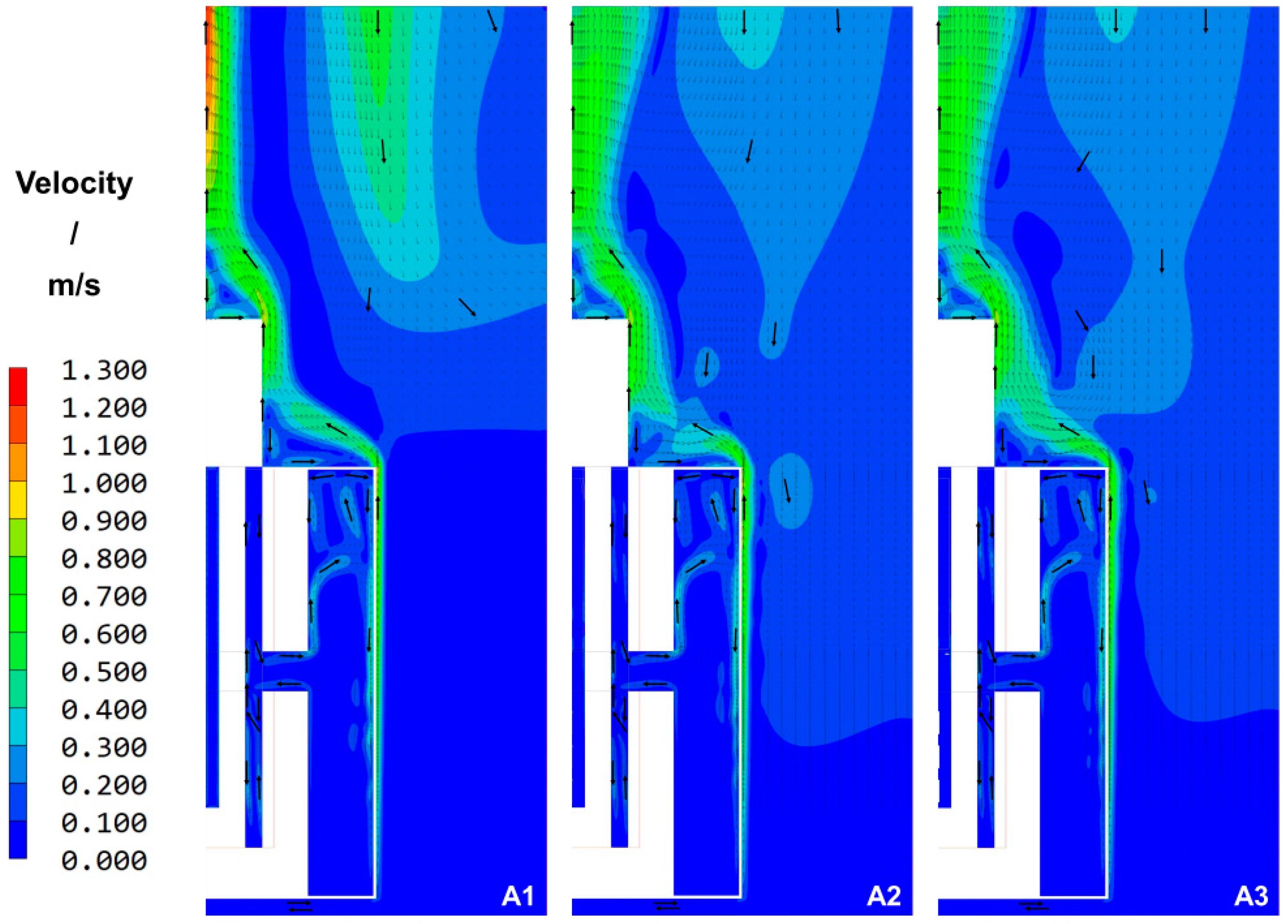
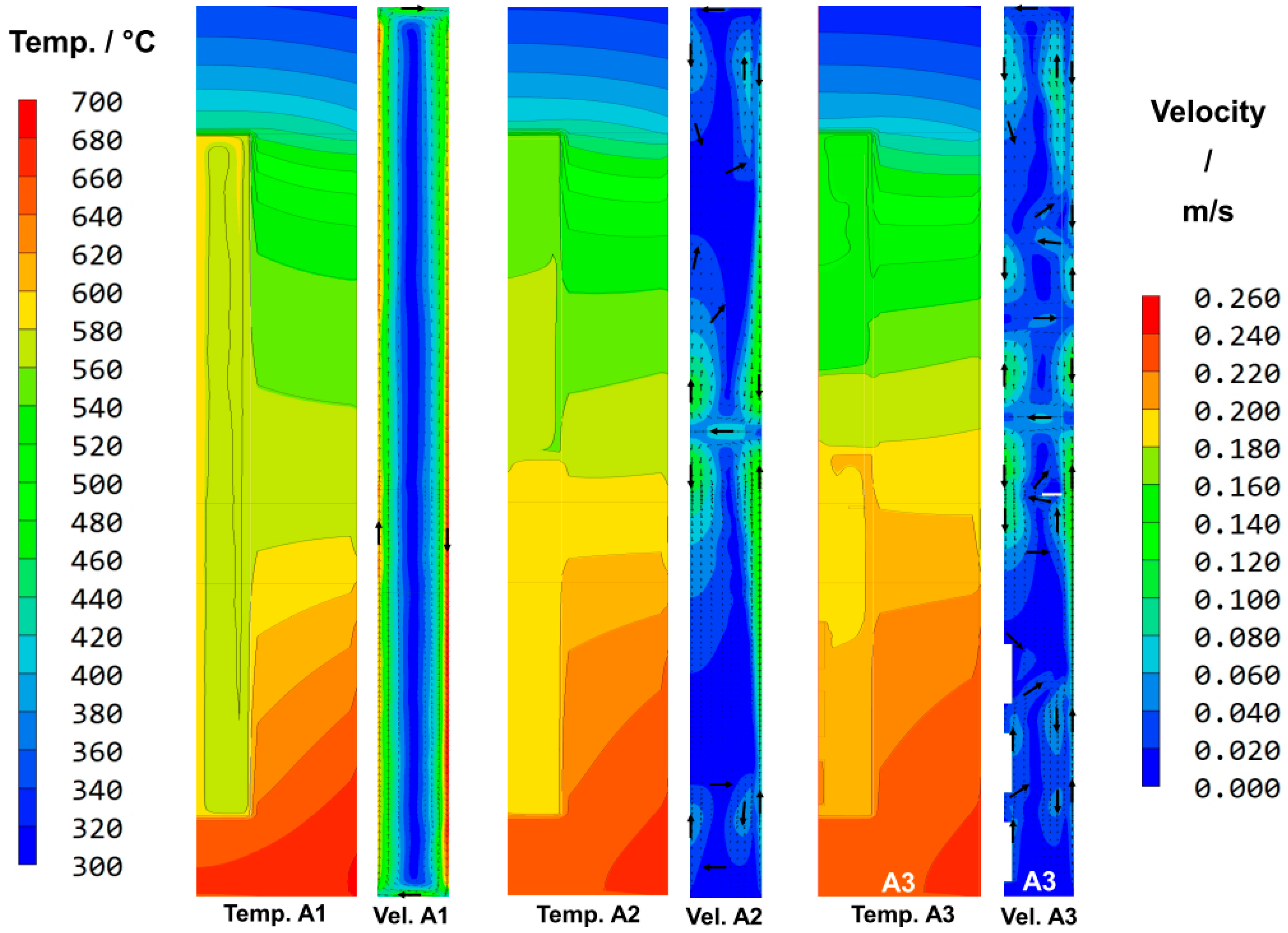
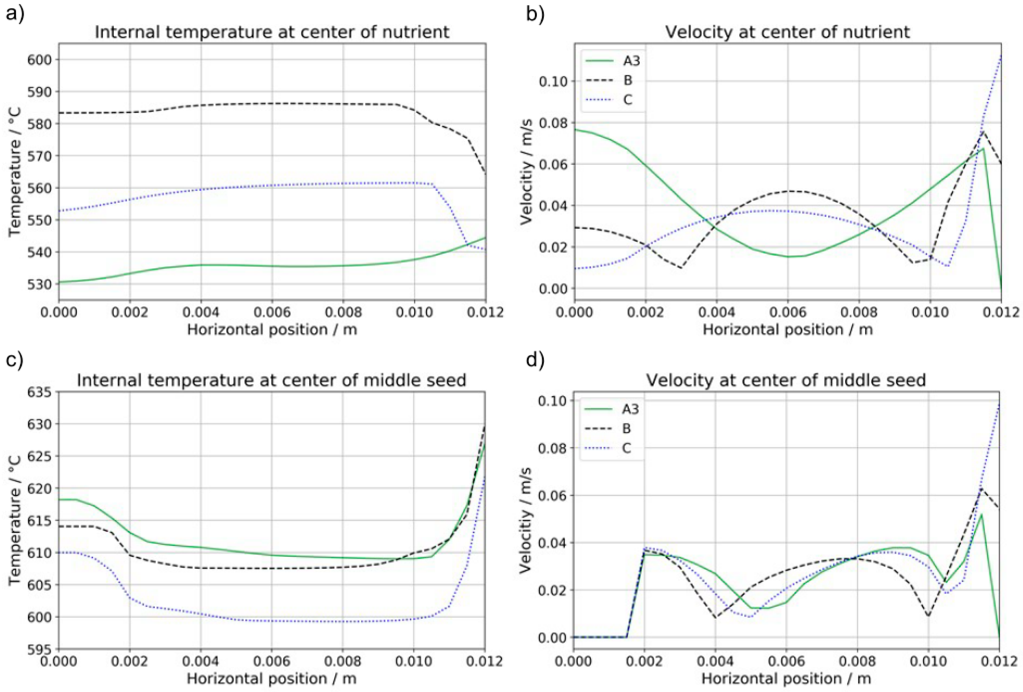
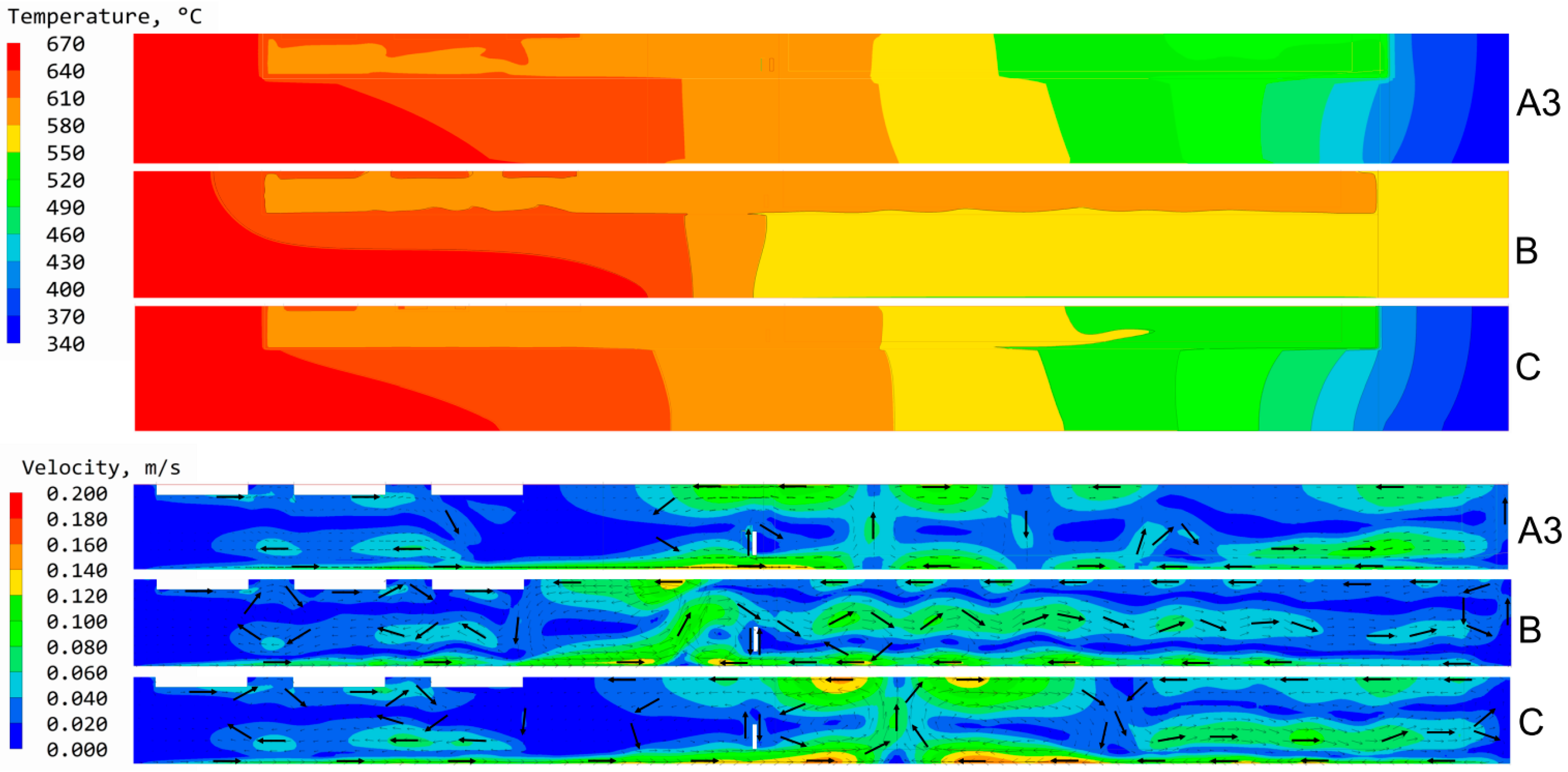
The model including the furnace was solved in three variations to investigate the impact of the flow model and the impact of solids inside the autoclave. The purpose of the geometry variation inside the autoclave was clarify how sensitively the wall temperature distribution reacts on changes in convective heat transfer inside the autoclave.

For comparison, the case closest to growth conditions (A3) was also simulated using the “conventional” method for boundary condition definition, i.e., including only the autoclave and with heater-long fixed temperatures and adiabatic walls elsewhere (B).

Lastly, the wall temperature distribution of case A3 was exported with a resolution of 0.5 mm and used as a boundary condition for an autoclave-only case termed case C. This was done in order to investigate the option of using a less complex geometry for detailed studies based on the wall temperature distribution obtained by the simulation including the furnace.

2.2. Machine Learning for Adjusting Input Parameters of Simulations

A complication for simulations using heater power as boundary condition is that it is difficult to directly simulate a case with specific set temperatures, as it is not known beforehand what power settings need to be used in order to reach (but not exceed) the specified set temperatures. In the following, the rate of heat supply to the heaters (or their output powers) will be termed $\dot{Q}$₁ and $\dot{Q}$₂, for the top and bottom heaters, respectively. Other quantities will carry subscripts 1 and 2 for the top and bottom zones as well. A combination of parametric runs and a machine learning model was used to accelerate the process of determining values for $\dot{Q}$₁ and $\dot{Q}$₂. The idea behind this is that for an otherwise given model, it may be possible to find a sufficiently accurate description of the relationship between heater powers and temperatures at the thermocouple locations that is much simpler and computationally less expensive than a simulation of heat transfer and fluid flow. 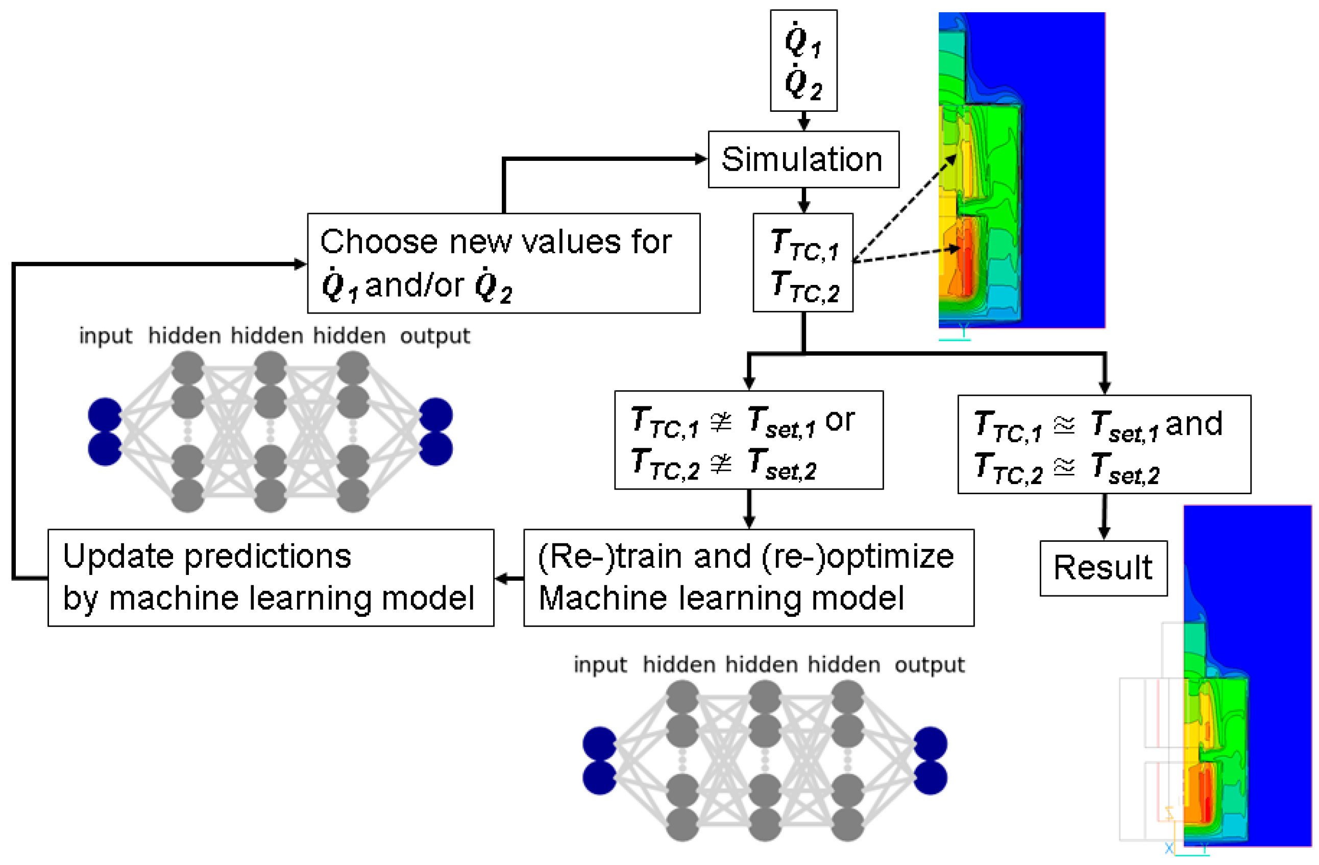Machine learning models using simulation results as input data have already been applied for modelling flow velocity and supersaturation in SiC solution growth, aiming at more efficient optimization of growth parameters [42]. This shows that fluid flow can be modelled relatively accurately using machine learning algorithms, suggesting that our approach for power tuning may also be feasible. Also, a machine learning model may be able to capture the effects of changes to the physical model studied by re-training on a relatively small number of simulations run with these variations as additional features. A flowchart visualizing the workflow of the integrated approach using both physics-based simulations and machine learning is depicted in Figure 2. The initial values for $\dot{Q}$₁ and $\dot{Q}$₂ need to be guessed well enough to produce a converging simulation while limiting temperatures to a physically reasonable range (20 °C to 3000 °C were used). Therefore, it can be necessary to do (or start and cancel if not converging due to exceeding the upper temperature limit) a few simulations initially. Once a rough estimate of the maximum power had been found, an evenly spaced grid of values was used to obtain more initial training data by conducting parametric runs. New values for $\dot{Q}$₁ and $\dot{Q}$₂ were chosen based on the predictions of the machine learning models. For this purpose, the models were used to predict temperatures T_TC,1 and T_TC,2 for 10,000 different power settings, which were created by generating two sets of random numbers and scaling them to the range of powers that had initially been found to be suitable for keeping temperatures in a reasonable range. From those predictions, 10 to 20 sets of power settings were chosen by searching for those that yield T_TC,1 and T_TC,2 closest to T_set,1 and T_set,2. These were then used in the next round of simulations (for technical reasons, the number of simulations that can be conducted within one parametric run depends on the number of digits of the parameters, hence the number had to be decreased when approaching the target values).

Machine learning models were programmed in Python using Tensorflow and scikit-learn software library. Both random forest regressor and a neural network models were tested. Due to the need to predict two temperatures (T_TC,1 and T_TC,2), MultiOutputRegressor was used when using models that do not natively support multiple outputs (random forest regressor). The number of features can be as low as two ($\dot{Q}$₁ and $\dot{Q}$₂) as long as the physics-based simulation considers only one model that does not vary except for the heater power settings. The model was initially trained on a subset of data with heater powers being the only two features, and subsequently re-trained as features had to be added and corresponding data became available.

Additional features (besides heater powers) comprise different open/space ratio of the baffle, number of seeds, nutrient porosity, and flow models. After adding new features, hyperparameters of the models were adapted in order to optimize accuracy. To make the process more time-efficient and also to make results regarding model accuracy more deterministic but keep the procedure efficient, hyperparameters that were found to have a significant influence in initial trials were optimized automatically by randomized search.

For the random forest regressor, mean absolute error was used as the criterion to evaluate the quality of a split. The most relevant parameters, which were then subject to automated hyperparameter optimization were the number of estimators and the maximum depth of the decision tree. For neural networks, the most relevant hyperparameters were the number and size of hidden layers and activation function, with the former two being the more important ones.

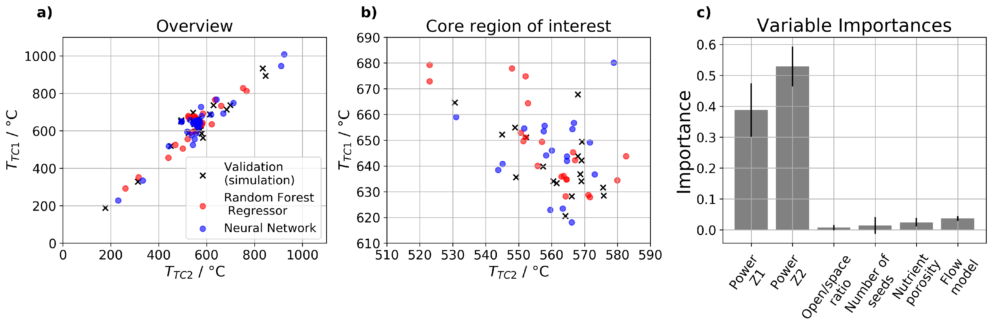
Although an extensive study of the developed machine learning algorithms is beyond the scope of this study, an overview on the performance of the models will be given. For this purpose, hyperparameters of models were optimized for a representative sample of typical datasets and the best obtained models were evaluated regarding their accuracy and training time. For evaluating the performance of the machine learning models as a function of dataset size (dataset group DG1 in

Table 5. Groups of datasets used for model evaluation. For the group that varies in the number of features (DG2), more detailed information is given in brackets in the following format: (Number of simulation datasets, number of features varying within these datasets).

Dataset Group	Varying Parameter	Parameter Values
DG1	Number of simulation data sets	10, 20, 30, 40, 50, 60, 70, 80, 90, 100, 110, 120, 130, 137
DG2	Number and types of features varying within dataset	No internal solids (54/3), no internal solids but only turbulent flow (59/3), all features but only laminar flow (50/5), all features but only turbulent flow (85/5)

), the order of the data was randomized prior to training in order to avoid unintentional co-evaluation of other factors affecting accuracy. Such factors could be specific to subsets of data containing only data with constant values for some of the features. An overview of groups of datasets used for evaluation is given in Table 5.

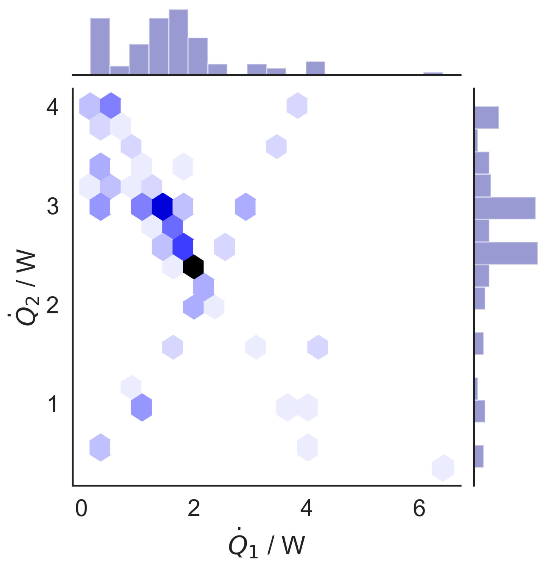
For the evaluation of the models, we will focus mainly on models using the resulting final dataset. This dataset will therefore be described and visualized in the following. An overview on the distribution of tested power settings (regardless of other features) is shown in Figure 3. The diagonal from low to high powers stems from the initial investigation to determine a suitable range of power settings. Since simulations subsequently focused on power settings resulting in temperatures close to the target values, the vicinity of those power settings is represented by more datapoints. While this may not be optimal for obtaining a model that generalizes well, it was sufficient for the purpose of the models in the current study.

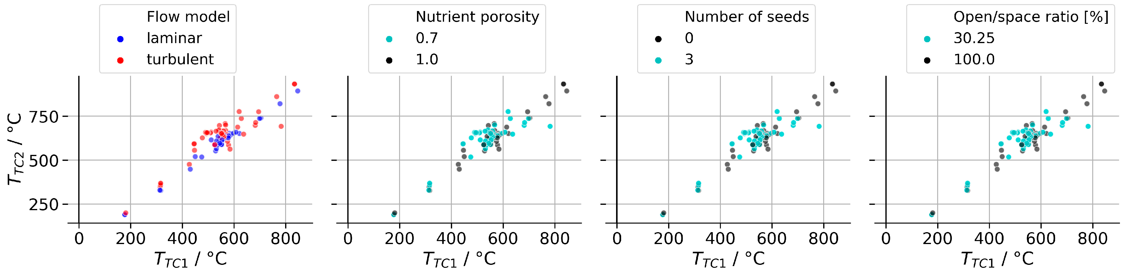
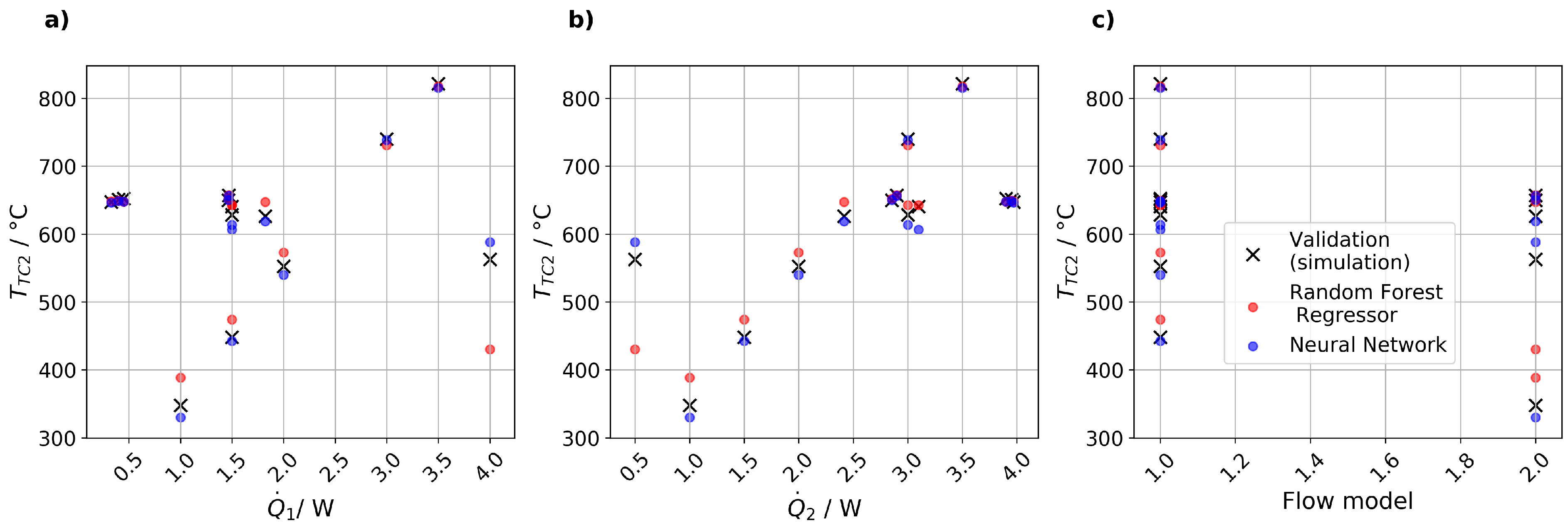
It is important to note that also the additionally features are not represented by equal amounts of data. This is visualized in Figure 4, which also shows the distribution of data as a function of control thermocouple temperatures. If plotted as a function of temperatures, the distribution of data exclusively follows a diagonal line (different from if plotted as a function of power settings). This indicates that both heaters have a significant effect on both zones. Comparing the subplots in Figure 4 shows that most simulations with laminar flow were done without internal solids such as nutrient, seeds and baffle. This is for two reasons: Firstly, laminar flow and an autoclave empty of solids were used for initial simulations for simplicity. Secondly, solids act as obstacles to flow and hereby increase the probability for the flow to be turbulent, thus, the combination of laminar flow with internal solids appears less likely to occur in reality. This distribution of data is not ideal from a machine learning perspective because it would be easier for a model to adequately capture the effects of all features if comprehensive data with all features varied independently were available. However, the objective here was to create data that are just good enough to find appropriate power settings reasonably quickly.

3. Results and Discussion

The methodic results regarding machine-learning-assisted simulations will be presented, followed by simulation results on outer autoclave wall temperature distribution. The effects of different boundary condition definition methods on the internal temperature and flow field results will be analyzed and the implications for future work will be discussed. First, result of the random forest regressor will be shown because this also allows for evaluating the relative importance of different features.

3.1. Results and Performance of Machine Learning Algorithms

Performance of a random forest regressor trained on the complete dataset at the end of this study is visualized in Figure 5a,b. It can be seen from Figure 5a that data from simulations are matched better in the region that contains most datapoints. Nevertheless, it is also clearly visible in Figure 5b that even in the core region of interest (i.e., vicinity of the targeted set temperatures), deviations are significant. Thus, the random forest regressor is most useful for initial rough estimation of a suitable power range to be studied in more detail, and for approximately quantifying feature importances. A bar diagram of feature importances (Mean Decrease in Impurity—see, e.g., [43] and references therein for a theoretical background on random forests and the related terminology) is presented in Figure 5c. The standard deviation of feature importances between the trees forming the forest (inter-trees variability) is displayed in the form of error bars in Figure 5c. The inter-trees variability suggests that both heater powers as well as the flow model have a statistically significant correlation with temperatures T_TC,1 and T_TC,2, whereas this is less clear for nutrient porosity. The number of seeds and open/space ratio do not show a clearly significant impact on the temperatures T_TC,1 and T_TC,2, thus we conclude that they have either no or only a weak influence on wall temperatures for a given combination of heater powers. It is interesting that the power of the bottom heater is recognized as a more important feature than the power of the top heater. This is a further indication of the importance of convective heat transfer, as convective heat transfer will cause heat transfer from the bottom to the top. This also fits well with a study by Li et al. [18] on industry scale hydrothermal autoclaves that views the bottom heater as the main heater and even assumes an outgoing heat flux for the autoclave wall in the region of the top heater.

Testing individually optimized neural networks for different sub-datasets (i.e., containing a reduced number of features or smaller amount of data, as dominant during data generation) shows that neural networks usually yielded a lower mean absolute error (or higher accuracy) compared to random forest regressors. Corresponding data are presented in

Table 6. Summary of typical data characterizing the accuracy and time-efficiency of random forest regressor and neural network models in this study. The term average indicates that values are an average of those for T_TC,1 and T_TC,2. The values in the table represent averages obtained using 19 datasets as described in Table 5.

Model Type	Mean Absolute Error (Average)/K	Mean Accuracy (Average)/%	Hyperparameter Optimization Time/min	Training Time (Best Estimator)/s
RFR	39.21 ± 19.89	92.61 ± 7.08	0.18 ± 0.34	1.19 ± 0.27
NN	14.94 ± 11.95	96.55 ± 3.44	11.28 ± 36.91	17.10 ± 19.50

. Though yielding better accuracy, neural networks also require more time for training and especially for the optimization of hyperparameters. The large standard deviation in both hyperparameter optimization and training times for neural network originate from the use of different activation functions, which strongly affects training times. In addition, the second investigated hyperparameter—number of hidden layers and numbers of neurons therein—also has a pronounced effect on training times. However, for the discussed task it is usually reasonable to invest the time needed to train neural networks.

The standard deviation for the average mean absolute errors indicate that there is a considerable variation depending on the number of features, amount of data per feature, and total amount of data for both types of models. However, trends behind such variations were not clearly observable due to the simultaneous variation of number of data and number of features.

An exemplary comparison of random forest regressor and neural network predictions in relation to simulation results is shown in Figure 6. Mean absolute errors in this example are 24.54 K for random forest regressor and 5.88 K for neural network, respectively. This comparison is for an intermediately complex (3 features) dataset of intermediate size (54 simulations). The neural network performs better especially when power settings of the two heaters are very different and seems to be better at capturing effects of turbulent flow. Nevertheless, the differences between the two models are less pronounced in the core area of interest (around T_TC,1 = 550 °C and T_TC,2 = 650 °C), which is probably due to a higher density of training data in that region. This higher density of data probably also is the reason that the accuracy of the models appears to be somewhat better in this core region of interest, thus, the errors and accuracies calculated for the entire data space underestimate the usefulness of the models. However, due to the high accuracy that would be desirable for the core region of interest both models were found to be most useful for speeding up the process of finding approximately suitable power settings. For finetuning (decreasing deviations from set temperatures from about 5 K to less than 1 K, manual adaptation of power settings was therefore sometimes found to be the easier path.

It is worth noting that although it is technically simple to create a model to directly predict heater powers for specified control thermocouple temperatures (i.e., using temperatures as a feature to predict corresponding power settings) this showed considerably worse results. A likely reason for this is that a combination of heater powers will deterministically result in a combination of temperatures T_TC,1 and T_TC,2 but a combination of temperatures can occur as a result of more than one combination of power settings. It was therefore more practical to use powers as features and make a large number of predictions for random power settings and select those that happened to come close to the desired temperatures for further consideration.

3.2. Results of Simulations That Include the Entire Growth Setup

An overview of the temperature distribution for the entire domain is shown in Figure 7 for cases A1, A2, and A3, respectively, and an analogous overview regarding the velocities is given in Figure 8. Note that the temperatures T_TC,1 and T_TC,2 for all evaluated type A cases deviate by only 0.3 K on average (maximum deviation: 0.9 K) and are thus deemed fully comparable for the purpose of this study. Specific values are denoted in Figure 8.

The adaptations in heater powers needed to reach near-identical temperatures at the control thermocouple locations is visible in the heater temperatures and the temperature distribution within the heaters. The trend of decreasing bottom heater temperature and increasing top heater temperature from A1 to A2 to A3 may be due to a decrease in convective heat transfer. From A1 to A2, the change from laminar to turbulent flow allows multiple, shorter convection cells to develop inside the autoclave whereas in case A1 there is only one convection cell with higher maximum velocities (see Figure 9 for a close-up of the interior space of the autoclave with adapted velocity scale).

In accordance with expectations, the velocity distribution in the air-filled spaces of the domain is very similar for all three cases (Figure 8). The higher maximum velocity above the autoclave head is likely due to more pronounced convective heat transfer inside the autoclave transporting heat to the autoclave head. Since the velocities are similar for all three cases in the air-filled spaces inside the furnace, it appears unlikely that there is a major direct effect of the flow model change on air flow and the related heat losses.

Regardless of the flow model and the presence or absence of solids inside the autoclave, inhomogeneous temperature distributions were found within each heater as well as within the corresponding sections of the autoclave wall (see Figure 9 for a close-up showing only the autoclave with an adapted temperature scale). It is worth noting that qualitatively similar inhomogeneities in wall temperatures within heater regions have also been found in numerical simulations of industry scale hydrothermal autoclaves [18], suggesting that wall temperature inhomogeneity occurs in a wide range of solvothermal reactors.

The wall temperature distribution remains qualitatively similar in all three cases. It is clearly evident that major heat losses through the uninsulated autoclave head have a strong effect on the temperature distribution in the autoclave wall that extends well into the region of the upper heater. This suggests that insulation or possibly even heating of the autoclave head could allow for improved control of temperature distribution and consequently supersaturation inside the autoclave. In terms of the fluid flow, there is a significant difference that affects internal temperature distribution: While laminar flow (in an autoclave empty of solids) results in a single convection cell and thus rather homogenous internal temperature distribution, multiple convection cells appear when turbulent flow is assumed. The occurrence of multiple convection cells can be related to the development of multiple regions that are characterized by more pronounced temperature differences and thus become visible in Figure 9. Expectably, this effect is fostered by the presence of solids, as they act as obstacles to flow and tend to cause a more complex flow consisting of an increasing number of smaller flow cells.

Isotherms through the autoclave walls are relatively close to horizontal in the upper half of the autoclave. Overall, it can be seen clearly that the thermal gradients in the outer autoclave wall are passed on to the inner wall and therefore must be expected to have a significant impact on the internal flow field. Slopes in isotherms through the autoclave wall appear to be caused by convective heat transfer inside the autoclave, resulting in opposite algebraic slope for the growth and dissolution zones, respectively.

A more detailed analysis of the temperature distribution at the outer autoclave walls is given in Figure 10, which shows profile plots of temperatures along all autoclave walls. Deviations between the different cases increase with increasing distance from the control thermocouple locations (labeled bottom/top heater setpoint in Figure 10). This is to be expected because heater powers were adjusted so as to create set temperatures at the locations where control thermocouples are located in the real experimental setup. For the vertical wall (Figure 10a), the length and position of the heaters is also indicated, and temperature distribution for heater-long fixed temperature boundary conditions are depicted schematically. This indicates that up to 50 K difference can occur at the outer autoclave wall depending on the method of boundary condition definition.

Regarding the top and bottom walls of the autoclave, the largest deviations occur between the two cases without interior solids. Deviations range from 8 K (bottom wall close to center) to 20 K (top inner wall close to center). This shows that convective heat transfer has a significant impact on the temperatures at autoclave head and bottom. This suggests that not only the flow model but also other assumptions that affect convective heat transfer (such as fluid properties) must be expected to have noticeable effects.

At the bottom of the autoclave, temperatures are higher at the outside and lowest at the center. This is in accordance with expectations because there are heat losses by convective heat transfer to the top and because these are less compensated further away from the heater. At the top of the autoclave, the opposite is observed, which is most likely due to a heating effect of warmer fluid rising as well as due to the geometry of the autoclave head (the distance to the nearest air-cooled head surface is longer at the center).

The general shape of the profile plots is similar in all cases, suggesting that it may be feasible to define boundary conditions as a location-dependent function that matches the set temperature at the control thermocouple locations.

3.3. Accuracy Losses with Conventional Boundary Condition Definitions

In the following, simulation case B will be analyzed in comparison to case A3. Case C is also plotted in the figures of this section for easier comparison but will be discussed in Section 3.4.

The comparison of case B and A3 shows that there are remarkable differences in the internal temperature distribution and velocity field depending on the method of boundary condition definition. As it can be seen in Figure 11a, there are major deviations in temperature distribution along the vertical direction at the centerline of the autoclave. Temperature deviations are most pronounced in the upper part of the autoclave and reach about 155 K near the top inner wall. This is likely to be relevant because the growth process is driven by the dependency of GaN solubility on temperature. Deviations in the growth zone are comparatively small (up to about 15 K) but could still have a noticeable effect. In particular, temperatures at seeds turns out to be more sensitive to seed position than a type B simulation would suggest. A thermal gradient between seeds at different height is in agreement with experimental results: There is usually an increase of growth rates towards the bottom of the autoclave.

In particular, the combination of a 15 K temperature deviation in the growth zone and a 60 K temperature deviation well within the nutrient can have large effects on the solubility difference between nutrient and seeds and therefore significant effects on growth rate must be expected. Experimental research with fluid temperature measurements near seeds and nutrient shows that the above-mentioned combination of temperature deviations can easily change growth rates by 100 µm/day in ammonothermal GaN growth using Na as mineralizer—the reader is encouraged to study Figure 2 in the referenced experimental study by Griffiths et al. [41].

As for the flow field (Figure 11b), results with both types of model are very similar in the vicinity of the seeds. However, type B simulation appears to exaggerate the flow velocity in the growth zone under the baffle and dampen local flow velocity fluctuations in the dissolution zone. Flow velocities in the dissolution zone are expected to affect dissolution kinetics, which in turn could have an impact on both on-seed growth and wall deposit formation.

In Figure 11c,d, temperatures and velocities in the vicinity of the inner wall are analyzed as a function of vertical position. The same general trends as already described for along the centerline are observed.

An analogous analysis for temperature and flow velocities in radial direction is presented in Figure 12 for two different vertical positions. Figure 12a,b refer to the vertical position at which the center of the nutrient is located, whereas Figure 12c,d refer to the vertical position of the center of the middle seed. As one may already suspect from the vertical profile line analyses, the temperature distributions in the growth zone show the same qualitative trends for all investigated boundary condition definitions (Figure 12c). Also, the radial distribution and magnitude of velocities is very similar in the growth zone (Figure 12d). However, as already indicated by the vertical plots, there are major deviations in the upper part of the autoclave. Figure 12a shows an inversion of the radial gradient, turning into a warm wall scenario for simulation A3. Note that the temperature scale in Figure 12a,c is rather different, thus, the deviations near the seeds shown in Figure 12c are not as large as they may seem at first. The radial distributions of velocities in the upper part of the autoclave is also rather different, although average magnitudes remain similar (see Figure 12b).

3.4. Refined Boundary Condition Definition Methods

A variety of adapted methods of boundary condition definition can now be envisioned. To balance computational cost and accuracy, it is of course desirable to work with a model that remains as small as possible, especially for detailed simulations of which many minor variations need to be computed. In the following, we investigate the option of working with a combination of type A simulations for determining the outer wall temperature distributions and a simplified simulation (type C) that uses the obtained outer wall temperature distribution as a boundary condition. The results of such a type C simulation are compared with those of a simulation that uses heater-long fixed set temperatures and adiabatic walls elsewhere (“conventional” boundary conditions, type B), as well as to type A simulation. Temperature distributions as well as flow fields of simulations with a typical set of internal solids as present during growth are shown in Figure 13 for all types of boundary condition definition.

As one can see from Figure 13, type C preserves the general characteristics that were observed in the corresponding simulation that included the furnace (A3), such as noticeable thermal gradients especially within the dissolution zone and the maximum velocities occurring further away from the seed crystals. For both A3 and C, the region where the two main convection cells meet resides inside the porous medium, in contrast to the result with heater-long fixed temperatures (B). This can be expected to have a major effect on mass transport during crystal growth. It should however be noted that more detailed studies that capture the variations of fluid flow speeds (and possibly flow pattern structure) over short and intermediate timescales need to be conducted in the future in order to fully evaluate which effects on crystal growth are to be expected. Capturing such short-term fluctuations was beyond the scope of this study, as the focus was to determine a realistic wall temperature distribution and suitable approach for future studies.

In view of the moderate sensitivity of outer wall temperatures to changes in flow obstacles or flow model (analyzed in Figure 10), we conclude that the considered stepwise approach can provide a reasonable balance of accuracy and computational cost, especially when further physical or chemical processes are to be included. This stepwise approach starts with a simulation using fixed heater power and including the furnace, with an internal geometry that should preferably be representative for an average of the internal geometries in the planned, more detailed studies. This outer wall temperature distribution can then be transferred to a simulation that includes only the autoclave, where it can be used as a fixed temperature boundary condition. This should be efficient as long as there are no frequent changes in set temperatures. In case of changing set temperatures, the process can be accelerated using machine learning for determining the appropriate power settings. Other ways to deal with frequent changes to set temperatures may be the numerical implementation of proportional–integral–derivative (PID) control or the definition of wall temperatures as a function of set temperatures and location based on the analysis of profile curve shapes of the temperature distribution. Such approaches are beyond the scope of this work but may be subject to future studies.

As for the computational cost, on the same workstation, case A3 took 3120 s of CPU time whereas B and C took 796 s and 457 s, respectively. It should be noted that the difference will become larger by various model modifications that have practical relevance for detailed studies of the internal flow. This includes anything that increases the computational cost per grid cell. In particular, simulations with high time resolution, 3D calculations, or simulations with added physics (such as supersaturation) are expected to be prohibitively time-consuming without limiting the domain to the autoclave for detailed studies.

4. Conclusions

The effect of different boundary condition assumptions on the internal temperature and fluid flow fields in ammonothermal autoclaves has been investigated directly for the first time. The results indicate that it is insufficient to use heater-long fixed temperatures at least if temperature distribution and fluid flow in the upper zone of the autoclave are also of interest. Deviations up to 155 K were observed at the upper end of the reaction chamber, which corresponds to the dissolution zone in the here investigated case of retrograde solubility. Clearly, this is a too large deviation if the dissolution process and local supersaturation are to be studied in a simulation. The observation that internal temperatures are affected by different types of boundary conditions especially in the upper part of the autoclave suggests that heat losses through the autoclave head are of significance. This suggests that insulation or direct temperature control through an additional heater may improve the controllability of internal temperature distribution and supersaturation. Depending on the boundary conditions there are also significant differences in flow pattern, in particular regarding the region in which the main convection cells meet. Especially for any simulation that includes mass transport of solutes, a more accurate way of defining thermal boundary conditions appears essential in view of these results. This holds in particular for simulations that implement local supersaturation as the driving force for ammonothermal crystallization, given that temperature deviations of about 60 K extend through much of the dissolution zone and add to temperature deviations of up to 15 K in the growth zone.

If growth and dissolution zones are inverted due to normal solubility, heat losses through the autoclave head can be expected to have an even more significant effect on the temperature distribution and fluid flow in the growth zone, since the growth zone is in the upper part of the autoclave in the case of normal solubility.

A first method for addressing the boundary condition problem was also presented. A balance between accuracy and computational cost can be achieved by combining two different models. The first model contains the furnace and its surrounding and uses heater powers as boundary conditions. This first model provides a realistic wall temperature distribution that is used as a fixed temperature boundary condition in the second model, which only includes the autoclave (including its walls). It is important to note that both models are conjugate in the sense that flow and temperature fields are solved simultaneously so that they can affect each other. This is necessary due to the importance of convective heat transfer.

For the practical problem of determining suitable power settings to match heater set temperatures, machine learning models and in particular neural networks can help to learn faster and more sustainably from past simulation experiences. Random forest regressors proved to be useful mostly at the beginning of the study when the amount of data was too small for neural networks to yield good accuracy; however, neural networks outperformed the random forest regressors as more data became available. Therefore, when applying this method on a regular basis with an increasing amount of data, neural networks are expected to yield better prediction accuracy as observed in the later parts of this study. However, random forest regressors remain useful even in the case of good data availability because they provide insights into the relative importance of different features. They can thus help to recognize features that do not show a statistically significant correlation with the target variables, which can be useful for example for implementing only relevant features in a neural network. Note, however, that it is important to select an appropriate measure of feature importance for the goals and data of a specific study (see for example [44] and references therein for an overview of established methods and recent developments in the variable importance evaluation of random forests). For both random forest regressors and neural networks, implementing automatic optimization of hyperparameters was found to be very helpful from the practical viewpoint of minimizing human trial-and-error efforts.

References

1. Eckert, C.A.; Knutson, B.L.; Debenedetti, P.G. Supercritical fluids as solvents for chemical and materials processing. Nature 1996, 383, 313–318. [Google Scholar] [CrossRef]
2. Häusler, J.; Schnick, W. Ammonothermal Synthesis of Nitrides: Recent Developments and Future Perspectives. Chem. A Eur. J. 2018, 24, 11864–11879. [Google Scholar] [CrossRef]
3. Sun, W.; Bartel, C.J.; Arca, E.; Bauers, S.R.; Matthews, B.; Orvañanos, B.; Chen, B.-R.; Toney, M.F.; Schelhas, L.T.; Tumas, W.; et al. A map of the inorganic ternary metal nitrides. Nat. Mater. 2019, 18, 732–739. [Google Scholar] [CrossRef] [Green Version]
4. Amano, H.; Baines, Y.; Beam, E.; Borga, M.; Bouchet, T.; Chalker, P.R.; Charles, M.; Chen, K.J.; Chowdhury, N.; Chu, R.; et al. The 2018 GaN power electronics roadmap. J. Phys. D. Appl. Phys. 2018, 51, 163001. [Google Scholar] [CrossRef]
5. Roccaforte, F.; Fiorenza, P.; Greco, G.; Lo Nigro, R.; Giannazzo, F.; Iucolano, F.; Saggio, M. Emerging trends in wide band gap semiconductors (SiC and GaN) technology for power devices. Microelectron. Eng. 2018, 187–188, 66–77. [Google Scholar] [CrossRef]
6. Sang, L.; Ren, B.; Sumiya, M.; Liao, M.; Koide, Y.; Tanaka, A.; Cho, Y.; Harada, Y.; Nabatame, T.; Sekiguchi, T.; et al. Initial leakage current paths in the vertical-type GaN-on-GaN Schottky barrier diodes. Appl. Phys. Lett. 2017, 111, 122102. [Google Scholar] [CrossRef]
7. Mikawa, Y.; Ishinabe, T.; Kagamitani, Y.; Mochizuki, T.; Ikeda, H.; Iso, K.; Takahashi, T.; Kubota, K.; Enatsu, Y.; Tsukada, Y.; et al. Recent progress of large size and low dislocation bulk GaN growth. In Proceedings of the Gallium Nitride Materials and Devices XV; Morkoç, H., Fujioka, H., Schwarz, U.T., Eds.; SPIE: Bellingham, DC, USA, 2020; Volume 1128002, p. 1. [Google Scholar]
8. Key, D.; Letts, E.; Tsou, C.-W.; Ji, M.-H.; Bakhtiary-Noodeh, M.; Detchprohm, T.; Shen, S.-C.; Dupuis, R.; Hashimoto, T. Structural and Electrical Characterization of 2′′ Ammonothermal Free-Standing GaN Wafers. Progress toward Pilot Production. Materials 2019, 12, 1925. [Google Scholar] [CrossRef] [PubMed] [Green Version]
9. Dwiliński, R.; Doradziński, R.; Garczyński, J.; Sierzputowski, L.P.; Puchalski, A.; Kanbara, Y.; Yagi, K.; Minakuchi, H.; Hayashi, H. Excellent crystallinity of truly bulk ammonothermal GaN. J. Cryst. Growth 2008, 310, 3911–3916. [Google Scholar] [CrossRef]
10. Pimputkar, S.; Kawabata, S.; Speck, J.S.S.; Nakamura, S. Improved growth rates and purity of basic ammonothermal GaN. J. Cryst. Growth 2014, 403, 7–17. [Google Scholar] [CrossRef]
11. Tomida, D.; Chichibu, S.F.; Kagamitani, Y.; Bao, Q.; Hazu, K.; Simura, R.; Sugiyama, K.; Yokoyama, C.; Ishiguro, T.; Fukuda, T. Improving the purity of GaN grown by the ammonothermal method with in-autoclave gas-phase acidic mineralizer synthesis. J. Cryst. Growth 2012, 348, 80–84. [Google Scholar] [CrossRef]
12. Tomida, D.; Bao, Q.; Saito, M.; Kurimoto, K.; Sato, F.; Ishiguro, T.; Chichibu, S.F. Effects of extra metals added in an autoclave during acidic ammonothermal growth of m -plane GaN single crystals using an NH 4 F mineralizer. Appl. Phys. Express 2018, 11, 091002. [Google Scholar] [CrossRef] [Green Version]
13. Masuda, Y.; Sato, O.; Tomida, D.; Yokoyama, C. Convection patterns and temperature fields of ammonothermal GaN bulk crystal growth process. Jpn. J. Appl. Phys. 2016, 55, 3–6. [Google Scholar] [CrossRef]
14. Erlekampf, J.; Seebeck, J.; Savva, P.; Meissner, E.; Friedrich, J.; Alt, N.S.A.; Schlücker, E.; Frey, L. Numerical time-dependent 3D simulation of flow pattern and heat distribution in an ammonothermal system with various baffle shapes. J. Cryst. Growth 2014, 403, 96–104. [Google Scholar] [CrossRef]
15. Jiang, Y.N.; Chen, Q.S.; Prasad, V. Numerical simulation of ammonothermal growth processes of GaN crystals. J. Cryst. Growth 2011, 318, 411–414. [Google Scholar] [CrossRef] [Green Version]
16. Mirzaee, I.; Charmchi, M.; Sun, H. Heat, mass, and crystal growth of GaN in the ammonothermal process: A numerical study. Numer. Heat Transf. Part A Appl. 2016, 70, 460–491. [Google Scholar] [CrossRef]
17. Chen, Q.S.; Pendurti, S.; Prasad, V. Effects of baffle design on fluid flow and heat transfer in ammonothermal growth of nitrides. J. Cryst. Growth 2004, 266, 271–277. [Google Scholar] [CrossRef] [Green Version]
18. Li, H.; Evans, E.A.; Wang, G.X. A three-dimensional conjugate model with realistic boundary conditions for flow and heat transfer in an industry scale hydrothermal autoclave. Int. J. Heat Mass Transf. 2005, 48, 5166–5178. [Google Scholar] [CrossRef]
19. Hashimoto, T.; Letts, E.; Hoff, S. Current Status and Future Prospects of Ammonothermal Bulk GaN Growth. Sens. Mater. 2013, 25, 155. [Google Scholar] [CrossRef]
20. Ferialdi, H.; Lappa, M.; Haughey, C. On the role of thermal boundary conditions in typical problems of buoyancy convection: A combined experimental-numerical analysis. Int. J. Heat Mass Transf. 2020, 159. [Google Scholar] [CrossRef]
21. Bao, Q.; Saito, M.; Hazu, K.; Furusawa, K.; Kagamitani, Y.; Kayano, R.; Tomida, D.; Qiao, K.; Ishiguro, T.; Yokoyama, C.; et al. Ammonothermal Crystal Growth of GaN Using an NH 4 F Mineralizer. Cryst. Growth Des. 2013, 13, 4158–4161. [Google Scholar] [CrossRef]
22. Bao, Q.; Saito, M.; Hazu, K.; Kagamitani, Y.; Kurimoto, K.; Tomida, D.; Qiao, K.; Ishiguro, T.; Yokoyama, C.; Chichibu, S.F. Ammonothermal growth of GaN on a self-nucleated GaN seed crystal. J. Cryst. Growth 2014, 404, 168–171. [Google Scholar] [CrossRef]
23. Spalding, D.B. The PHOENICS Encyclopaedia, Concentration, Heat and Momentum Limited (CHAM), London, UK. Available online: http://www.cham.co.uk/phoenics/d_polis/d_enc/encindex.htm (accessed on 3 March 2021).
24. Lemmon, E.W.; McLinden, M.O.; Friend, D.G. Thermophysical Properties of Fluid Systems; Linstrom, P.J., Mallard, W.G., Eds.; NIST Chemistry WebBook. NIST Standard Reference Database Number 69; National Institute of Standards and Technology: Gaithersburg, MD, USA. Available online: http://webbook.nist.gov/chemistry (accessed on 5 June 2017).
25. Spalding, B. Trends, Tricks, and Try-ons in CFD/CHT, 1st ed.; Elsevier: Amsterdam, The Netherlands, 2013; Volume 45, ISBN 9780124078192. [Google Scholar]
26. Alt, N.; Meissner, E.; Schlücker, E.; Frey, L. In situ monitoring technologies for ammonthermal reactors. Phys. Status Solidi Curr. Top. Solid State Phys. 2012, 9, 436–439. [Google Scholar] [CrossRef]
27. Chen, Q.-S.; Jiang, Y.-N.; Yan, J.-Y.; Li, W.; Prasad, V. Modeling of ammonothermal growth processes of GaN crystal in large-size pressure systems. Res. Chem. Intermed. 2011, 37, 467–477. [Google Scholar] [CrossRef] [Green Version]
28. Lin, Y.S.; Akins, R.G. A Suggested Characteristic Dimension for Natural Convection in Enclosures. Chem. Eng. Commun. 1986, 49, 119–126. [Google Scholar] [CrossRef]
29. Krishnamurti, R. Some further studies on the transition to turbulent convection. J. Fluid Mech. 1973, 60, 285–303. [Google Scholar] [CrossRef]
30. Schimmel, S.; Duchstein, P.; Steigerwald, T.G.; Kimmel, A.-C.L.; Schlücker, E.; Zahn, D.; Niewa, R.; Wellmann, P. In situ X-ray monitoring of transport and chemistry of Ga-containing intermediates under ammonothermal growth conditions of GaN. J. Cryst. Growth 2018, 498, 214–223. [Google Scholar] [CrossRef]
31. Masuda, Y.; Suzuki, A.; Mikawa, Y.; Yokoyama, C.; Tsukada, T. Numerical simulation of natural convection heat transfer in a ZnO single-crystal growth hydrothermal autoclave—Effects of fluid properties. J. Cryst. Growth 2009, 311, 675–679. [Google Scholar] [CrossRef]
32. Pendurti, S.; Chen, Q.S.; Prasad, V. Modeling ammonothermal growth of GaN single crystals: The role of transport. J. Cryst. Growth 2006, 296, 150–158. [Google Scholar] [CrossRef] [Green Version]
33. Masuda, Y.; Suzuki, A.; Ishiguro, T.; Yokoyama, C. Heat and Fluid Flow in Solvothermal Autoclave for Single-Crystal Growth Process. J. Therm. Sci. Technol. 2012, 7, 379–386. [Google Scholar] [CrossRef] [Green Version]
34. Masuda, Y.; Suzuki, A.; Ishiguro, T.; Yokoyama, C. Numerical Simulation of Heat and Fluid Flow in Ammonothermal GaN Bulk Crystal Growth Process. Jpn. J. Appl. Phys. 2013, 52, 08JA05. [Google Scholar] [CrossRef]
35. Masuda, Y.; Suzuki, A.; Mikawa, Y.; Kagamitani, Y.; Ishiguro, T.; Yokoyama, C.; Tsukada, T. Numerical simulation of GaN single-crystal growth process in ammonothermal autoclave—Effects of baffle shape. Int. J. Heat Mass Transf. 2010, 53, 940–943. [Google Scholar] [CrossRef]
36. Mirzaee, I. Computational investigation of gallium nitrite ammonothermal crystal growth. In Proceedings of the ASME 2013 Heat Transfer Summer Conference collocated with the ASME 2013 7th International Conference on Energy Sustainability and the ASME 2013 11th International Conference on Fuel Cell Science, Engineering and Technology, Minneapolis, MN, USA, 14–19 July 2015. [Google Scholar]
37. Schimmel, S.; Kobelt, I.; Heinlein, L.; Kimmel, A.L.; Steigerwald, T.G.; Schlücker, E.; Wellmann, P. Flow Stability, Convective Heat Transfer and Chemical Reactions in Ammonothermal Autoclaves—Insights by In Situ Measurements of Fluid Temperatures. Crystals 2020, 10, 723. [Google Scholar] [CrossRef]
38. Spalding, D.B. A single formula for the “law of the wall”. J. Appl. Mech. Trans. ASME 1960, 28, 455–458. [Google Scholar] [CrossRef]
39. Ludwig, J.C. PHOENICS-VR Reference Guide 2011; CHAM: London, UK, 2011; pp. 1–249. [Google Scholar]
40. Diethelm, K. The limits of reproducibility in numerical simulation. Comput. Sci. Eng. 2012, 14, 64–72. [Google Scholar] [CrossRef]
41. Griffiths, S.; Pimputkar, S.; Kearns, J.; Malkowski, T.F.; Doherty, M.F.; Speck, J.S.; Nakamura, S. Growth kinetics of basic ammonothermal gallium nitride crystals. J. Cryst. Growth 2018, 501, 74–80. [Google Scholar] [CrossRef]
42. Tsunooka, Y.; Kokubo, N.; Hatasa, G.; Harada, S.; Tagawa, M.; Ujihara, T. High-speed prediction of computational fluid dynamics simulation in crystal growth. CrystEngComm 2018, 20, 6546–6550. [Google Scholar] [CrossRef] [Green Version]
43. Breiman, L. Random Forests. Mach. Learn. 2001, 45, 5–32. [Google Scholar] [CrossRef] [Green Version]
44. Loecher, M. Unbiased variable importance for random forests. Commun. Stat. Theory Methods 2020, 1–13. [Google Scholar] [CrossRef]
Figure 1. Geometry and materials used in simulation of temperature distribution and fluid flow. (a) Domain of type A cases, with fluid regions indicated by color (blue: Air, red: Supercritical NH3). The distance between bottom domain boundary and bottom of the furnace is 15 mm, (b) Close-up of geometry showing the solid materials. The red areas correspond to the two heaters. (c) Simulation domain, geometry, and materials for cases of type B and C, containing only the autoclave and its interior. X, Y, and Z represent the positive directions of the cartesian coordinate system used to describe the geometry in the simulation. Gravity acts in the negative Z direction.
Crystals 11 00254 g001
Figure 2. Workflow using for machine-learning assisted power adjustment in simulations.
Crystals 11 00254 g002
Figure 3. Overview of the distribution of data with different power settings in the final dataset. Darker color corresponds to a higher amount of datapoints in the respective region, as also indicated by the bar plots.
Crystals 11 00254 g003
Figure 4. Overview of generated simulation data. Data are split by different features in the subplots as indicated by the legends. Darker regions indicate overlap of datapoint symbols. Cyan symbols represent cases with internal solids, black datapoints indicate cases without solids inside the autoclave.
Crystals 11 00254 g004
Figure 5. Results using the complete dataset at the end of this study. (a) Overview of simulated data together with those predicted by the random forest regressor and neural network, (b) close-up of the temperature region of interest, (c) feature importances obtained from the random forest regressor model (error bars represent inter-trees variability).
Crystals 11 00254 g005
Figure 6. Exemplarily comparison of prediction data from random forest regressor and neural network to test data. (a) Bottom temperature TTC,2 as a function of top power Q ˙ 1, (b) bottom temperature TTC,2 as a function of bottom power Q ˙ 2, (c) splitting of the data by the third feature, namely flow model.
Crystals 11 00254 g006
Figure 7. Overview of temperature distribution in the entire domain for cases A1, A2, and A3, respectively. A brief description of the characteristics of each case is given in the insets at the top.
Crystals 11 00254 g007
Figure 8. Overview of velocity distribution in the entire domain for cases A1, A2, and A3, respectively. For better visibility, thick arrows were added as guides to the eye.
Crystals 11 00254 g008
Figure 9. Close-ups showing the temperature distribution in the walls and interior of the autoclave (left subfigure of each case) and velocity distribution inside the autoclave (right subfigure of each case). For better visibility, thick arrows were added as guides to the eye.
Crystals 11 00254 g009
Figure 10. Temperature distributions at outer autoclave walls determined by simulations of the complete setup including the furnace. (a) Vertical autoclave wall. (b) Horizontal autoclave walls (horizontal position of 0 corresponds to symmetry axis of autoclave). For the top autoclave wall, a position in the autoclave head corresponding to the thickness of the bottom autoclave wall was chosen, as this mimics a suitable choice for simulations that do not include the furnace.
Crystals 11 00254 g010
Figure 11. Comparison of internal temperatures (a,c) and flow velocities (b,d) depending on the method of boundary condition definition along the centerline of the autoclave (a,b) and in the vicinity of the inner autoclave wall (c,d). Regions with zero velocity originate from fully blocking solids.
Crystals 11 00254 g011
Figure 12. Comparison of internal temperatures (a,c) and flow velocities (b,d) depending on the method of boundary condition definition in radial direction at the center of the nutrient (a,b) and at the center of the middle seed (c,d). Regions with zero velocity originate from fully blocking solids.
Crystals 11 00254 g012
Figure 13. Temperature distributions (top) and flow fields (bottom) for case type A (including furnace and surrounding), B (heater-long fixed temperature), and type C (i.e., using the outer wall temperature distribution extracted from the corresponding furnace-including simulation A3). The plots of the velocity fields have been changed in aspect ratio to improve readability of the figure, and the figures are rotated with respect to gravity (bottom of the autoclave is on the left side of the figure). For better visibility, thick arrows were added as guides to the eye.
Crystals 11 00254 g013