Article

Theoretical Model for a Novel Electronic State in a Dirac Electron System Close to Merging: An Imaginary Element between Sulphur and Selenium

by
Toshio Naito
1,2,3,* and
Yoshikazu Suzumura
4
1
Graduate School of Science and Engineering, Ehime University, Matsuyama 790-8577, Japan
2
Research Unit for Development of Organic Superconductors, Ehime University, Matsuyama 790-8577, Japan
3
Geodynamics Research Center (GRC), Ehime University, Matsuyama 790-8577, Japan
4
Department of Physics, Nagoya University, Nagoya 464-8602, Japan
*
Author to whom correspondence should be addressed.
Submission received: 11 February 2022 / Revised: 27 February 2022 / Accepted: 28 February 2022 / Published: 2 March 2022
(This article belongs to the Special Issue Organic Conductors)

Abstract

:
Topological materials with Dirac electron systems have been extensively studied. Organic crystalline materials form a unique group of such compounds with well-defined crystal structures. While most organic compounds require high pressures to exhibit Dirac-cone-type band structures, the title compound, α-STF2I3, has garnered increasing interest due to its Dirac-cone-type band structure under ambient pressure. Various experiments have been conducted under ambient pressure; their results can be compared with those of theoretical calculations to obtain insights into Dirac electron systems. However, structural disorder peculiar to the STF molecules in the solid-state has prevented any type of theoretical calculation of the states. In this study, we report a new method for calculating intermolecular interactions in disordered systems based on the extended Hückel approximation. This method enables band calculations, suggesting that this material is a rare example of a system close to merging. The obtained band structure indicates that the characteristic disorder in the STF solids distributed electrons equally on the sulphur and selenium atoms as if they belong to an imaginary element between sulphur and selenium and are arranged without disorder.

1. Introduction

Recently, Dirac electron systems (DESs), which are characterised by massless relativistic electrons with speeds of 1/100–1/1000th of the velocity of light, have been widely studied. The majority of the studies on DESs are theoretical because of the limited availability of DES materials [1,2,3,4,5,6,7,8,9]. Concerning the general molecular systems, the electronic structures including those under high pressure are calculated by DFT methods [10,11,12]. Although DESs were initially found in graphene [13,14] and some inorganic compounds [15], those found in organic compounds [16] possess clear advantages over their inorganic counterparts. For example, most organic DESs are found in bulk systems with well-defined crystal structures and chemical stoichiometries, whereas inorganic DESs often lack either of these two features. However, organic DESs have some disadvantages; for example, most become DES only under high pressure [17,18,19,20], unlike inorganic DESs. Performing detailed, accurate experiments and measurements (including crystal structure analyses) at high pressures is more complicated than those at ambient pressure. In this regard, the organic charge-transfer (CT) complex, α-STF2I3 (Figure 1; STF = bis(ethylenedithio)-diselenadithiafulvalene), is unique as it contains Dirac electrons at ambient pressure [21,22,23,24,25,26]; that is, it possesses the advantages of both organic and inorganic DESs.
All the electrical, magnetic, and optical properties of the DESs are governed by the intermolecular interactions between the STF molecules in α-STF2I3. In principle, intermolecular interactions, band structures, and various physical properties of crystalline materials can be calculated when all the atomic positions, namely atomic parameters, are known, assuming perfect three-dimensional periodic arrangements of the atoms in the framework of well-established band theories. However, it is challenging to calculate the intermolecular interactions, that is, the overlap and transfer integrals between the STF molecules in α-STF2I3, because all the STF molecules in this CT complex are randomly disordered between the two patterns shown in Figure 2. The calculations of the electronic structures and related quantities in the solid states require well-defined atomic parameters for all the atoms involved. Although DES materials with the disorder are seldom reported and have garnered considerable attention [27,28,29], the lack of the abovementioned calculation results has seriously hindered further studies on this CT complex and a clear understanding of the general DESs.
We have recently proposed a tight-binding band structure of α-STF2I3 based on the overlapping integrals SSTF, assuming statistically averaged structures between all the possible molecular arrangements at each site in the disordered crystal (Figure 3; see Appendix A for details) in addition to the assumption of tSTF/eV = −10SSTF, where tSTF represents the corresponding transfer integrals [21]. The band structure obtained in our previous study was characterised by less tilted and more isotropic Dirac cones compared to that in the present study.
The calculated band structure failed to reproduce the observed anisotropic temperature dependence of resistivity, despite being qualitatively consistent with the nearly temperature-independent electrical resistivity. In this paper, we propose a new method based on molecular orbitals (MOs) to estimate the overlap and transfer integrals in such disordered systems more clearly. More importantly, we found that solid-state STF molecules form unique electron configurations, which are qualitatively different from those in other disordered crystalline materials. The differences between the STF solids and other disordered systems include observed qualitative differences in electrical, magnetic, spectroscopic, and structural properties. The STF solids almost always behave as if there is no disorder in their crystal structures. In contrast, the slightest disorder frequently alters qualitative behaviours compared with those of related or corresponding materials without the disorder in common crystalline materials. To explain this fact, we propose a new idea of wavefunctions analogous to molecular orbitals and based on the original meanings of wavefunctions.

2. Calculation Methods

Single-crystal X-ray structural analyses demonstrated that all four chalcogen atoms (X: Figure 2) in the solid-state STF molecules possessed equal electron densities [21,22,23,24,25,26]. This trend is not only the case with conducting STF CT complexes, but also the case with insulating STF CT complexes and even with the neutral STF molecular crystals, irrespective of the crystal structures and the molecular symmetries required for the positions in the unit cells [26]. This trend is peculiar to the STF molecule in the solid-state, which cannot be explained by the known quantum stabilisation effects, such as delocalisation or intermolecular interactions. Such electron configurations require that all the atomic positions and the electron densities on each X atom are fixed in each molecule, regardless of the packing pattern. Thus, only the degrees of freedom remain in the assignment of S and Se atoms at fixed X positions with equal electron densities. In other words, the electron densities were averaged for all four X atoms as if the X atoms belonged to imaginary element between sulphur and selenium. This is probably because the differences in the atomic energy levels are sufficiently small between S and Se atoms, favouring such averaged electron configuration. Ultimately, this configuration would lead to the reduction of Coulombic repulsion between electrons, in addition to stabilisation due to the increased kinetic energy of electrons. As wavefunctions for electrons are associated with electron densities, we assumed that the wavefunction of an STF molecule (Equation (1)) in the solid state (ϕSTF (MO of STF)) should be described using the two wavefunctions corresponding to the average of the two patterns in Figure 2.
ϕ STF = 1 2 ϕ 1 + 1 2 ϕ 2
where suffixes 1 and 2 denote the different patterns shown in Figure 2. To equally distribute the electrons on the X atoms in the STF molecules, both coefficients must be equal, that is, 1 / 2 if Equation (1) is normalised and if the cross-terms are ignored. The cross-terms between ϕ 1 and ϕ 2 are ignored because the two orientations ( ϕ 1 and ϕ 2) never coincide at a given site for a single STF molecule. In other words, such an averaged electron configuration does not involve the exchange or oscillating movement between the S and Se nuclei in the STF molecules. Equation (1) describes the electronic configuration of the X atoms in Figure 2, corresponding to the imaginary element between S and Se. Notably, it appears that Equation (1) describes the interaction between the two states or the fluctuation originating from the quantum interference between the two states. However, this is not the case. As we will see by substituting atomic orbitals in Equation (1), a “conjugate” equation, that is, a state corresponding to Equation (2) does not describe the electronic configuration of the solid STF molecules (Equation (6)).
ϕ STF = 1 2 ϕ 1 1 2 ϕ 2
All the wavefunctions below are assumed to be normalised. We use the same coefficients even after altering the expression, except when it is misleading.
The molecular orbital ϕ i (i = 1, 2) was substituted into Equation (1) through a linear combination of atomic orbitals, φ j ,
ϕ i = j c j φ j
where cj and φ j denote the coefficient and atomic orbital of atom j, respectively. For example, φ H designates the 1s orbital of a hydrogen atom. For j = C (carbon), φ j should describe one of the C 1s, C 2s, C 2px, C 2py, and C 2pz orbitals. Note that all the atomic positions, except for the X atoms, r j , and electron densities on all the atoms in an STF molecule are common between ϕ 1 and ϕ 2 .
The molecular orbitals ϕ i (i = 1, 2) obtained in this way are as follows:
ϕ 1 = j a Y φ Y ( r J ) + k b S φ S ( r k ) + l c Se φ Se ( r l )
ϕ 2 = j a Y φ Y ( r J ) + k b Se φ Se ( r k ) + l c S φ S ( r l )
where suffixes j, k, and l indicate the atomic positions in the STF molecule. Suffix Y indicates atoms other than X atoms in the STF molecule. Notably, the first terms in Equations (4) and (5) are identical. Meanwhile, the coordinates r k and r l for S and Se atoms indicate the X atoms on the left and right sides of each STF molecule, respectively. Accordingly, the two equations of ϕ 1 and ϕ 2 are identical, except for the coordinates r k and r l for S and Se atoms (the position vectors in real space for X atoms), respectively. By substituting Equations (4) and (5) in Equation (2), we obtain
ϕ STF = 1 2 ϕ 1 1 2 ϕ 2 = 1 2 { k b S φ S ( r k ) + l c Se φ Se ( r l ) } 1 2 { k b Se φ Se ( r k ) + l c S φ S ( r l ) }
which evidently does not describe the electronic configuration required for the solid STF molecules.
By substituting Equations (4) and (5) in Equation (1), we obtain
ϕ STF = 1 2 { j a Y φ Y ( r J ) + k b S φ S ( r k ) + l c Se φ Se ( r l ) } + 1 2 { j a Y φ Y ( r J ) + k b Se φ Se ( r k ) + l c S φ S ( r l ) } = 1 2 { j a Y φ Y ( r J ) + k b S φ S ( r k ) + l c S φ S ( r l ) } + 1 2 { j a Y φ Y ( r J ) + k b Se φ Se ( r k ) + l c Se φ Se ( r l ) }
Therefore,
ϕ STF = 1 2 ϕ ( X = S ) + 1 2 ϕ ( X = Se )
where ϕ ( X = S ) and ϕ ( X = Se ) represent the following MOs, respectively.
ϕ ( X = S ) = j a Y φ Y ( r J ) + k b S φ S ( r k ) + l c S φ S ( r l )
ϕ ( X = Se ) = j a Y φ Y ( r J ) + k b Se φ Se ( r k ) + l c Se φ Se ( r l )
In short, ϕ ( X = S ) and ϕ ( X = Se ) are molecular orbitals, assuming that all the X atoms in Figure 2 should be either S or Se atoms with identical atomic positions, respectively. As such, the wavefunctions (MOs) of disordered solid-state STF molecules can be described by the equal contributions of the MOs of ϕ ( X = S ) and ϕ ( X = Se ) , as shown in Equation (8).
Next, we discuss the electron densities of the STF sites in the solid state using Equation (8). The contribution of MO, ϕ STF , to the electron densities of a given STF site in a solid state is described as follows:
2 | ϕ STF | 2 d V = 2 ( 1 2 ϕ ( X = S ) + 1 2 ϕ ( X = Se ) ) * ( 1 2 ϕ ( X = S ) + 1 2 ϕ ( X = Se ) ) d V = ( | ϕ ( X = S ) | 2 d V + | ϕ ( X = Se ) | 2 d V ) + ( ϕ ( X = Se ) * ϕ ( X = S ) d V + ϕ ( X = S ) * ϕ ( X = Se ) d V )
where the integral is calculated over the entire space. The coefficient “2” is required by spin multiplicity. Thus, by noting that ϕ STF , ϕ ( X = S ) , and ϕ ( X = Se ) are normalised,
2 = 2 + ( ϕ ( X = Se ) * ϕ ( X = S ) d V + ϕ ( X = S ) * ϕ ( X = Se ) d V )
Then,
ϕ ( X = Se ) * ϕ ( X = S ) d V + ϕ ( X = S ) * ϕ ( X = Se ) d V = 0
In other words,
| ϕ STF | 2 d V = 1 2 ( | ϕ ( X = S ) | 2 d V + | ϕ ( X = Se ) | 2 d V )
Equation (13) indicates that the electron densities of disordered STF molecules can be described by the average of the electron densities of the ϕ ( X = S ) and ϕ ( X = Se ) eigenstates, consistent with the observations.
The discussion thus far indicates that intermolecular interactions between disordered STF molecules in the solid state can be described by replacing the wavefunction of STF, ϕ STF , with an average of the wavefunctions of ϕ ( X = S ) and ϕ ( X = Se ) (Equation (8)). In disordered STF CT complexes, one can similarly calculate the overlap (S) and transfer (t) integrals between STF molecules based on Equation (8). The overlap ( S STF ) and transfer ( t STF ) integrals between two STF molecules located at R 1 and R 2 , respectively, are:
S STF = ϕ STF ( R 1 ) ϕ STF ( R 2 ) d V = ( 1 2 ϕ ( X = S ) ( R 1 ) + 1 2 ϕ ( X = Se ) ( R 1 ) ) * ( 1 2 ϕ ( X = S ) ( R 2 ) + 1 2 ϕ ( X = Se ) ( R 2 ) ) d V   ( Equation   ( 8 ) ) 1 2 { ϕ ( X = S ) ( R 1 ) ϕ ( X = S ) ( R 2 ) d V + ϕ ( X = Se ) ( R 1 ) ϕ ( X = Se ) ( R 2 ) d V } = 1 2 { S ( X = S ) + S ( X = Se ) } ,
where
S ( X = S ) = ϕ ( X = S ) ( R 1 ) ϕ ( X = S ) ( R 2 ) d V
S ( X = Se ) = ϕ ( X = Se ) ( R 1 ) ϕ ( X = Se ) ( R 2 ) d V
If the cross terms are ignored (Equation (17)):
ϕ ( X = Se ) * ( R 1 ) ϕ ( X = S ) ( R 2 ) d V + ϕ ( X = S ) * ( R 1 ) ϕ ( X = Se ) ( R 2 ) d V = 0
The validity for Equation (17) is discussed after deriving the transfer integrals. Similarly,
t STF = ϕ STF ( R 1 ) H ^ ϕ STF ( R 2 ) d V = 1 2 { E ( X = S ) S ( X = S ) + E ( X = Se ) S ( X = Se ) } + 1 2 { E ( X = Se ) ϕ ( X = S ) ( R 1 ) ϕ ( X = Se ) ( R 2 ) d V + E ( X = S ) ϕ ( X = Se ) ( R 1 ) ϕ ( X = S ) ( R 2 ) d V }                     ( Equation ( 14 ) )
where E(X = S) and E(X = Se) are the energies of the orbitals of interest, for example, the HOMO. Below, we limit our discussion to the HOMO of an STF molecule, which dominates the physical properties of α-STF2I3.
H ^ ϕ ( X = S ) = E ( X = S ) ϕ ( X = S ) ,     H ^ ϕ ( X = Se ) = E ( X = Se ) ϕ ( X = Se ) ,
Therefore, Equation (18) is further altered to
t STF = 1 2 { t ( X = S ) + t ( X = Se ) } ,
where
t ( X = S ) = E ( X = S ) S ( X = S ) ,   t ( X = Se ) = E ( X = Se ) S ( X = Se )
and we approximated
E ( X = Se ) ϕ ( X = S ) ( R 1 ) ϕ ( X = Se ) ( R 2 ) d V + E ( X = S ) ϕ ( X = Se ) ( R 1 ) ϕ ( X = S ) ( R 2 ) d V 0
E ( X = Se ) E ( X = S ) = 10   ( eV )

3. Results and Discussion

The obtained SSTF overlap integrals are listed in Table 1. Figure 4 shows the interacting pairs of the STF molecules corresponding to the SSTF values in Table 1.
The validities of Equations (17) and (22) were not proven in this general discussion. However, the derived parameters, SSTF (Table 1) and tSTF, semi-quantitatively reproduced the observed electrical properties. In contrast, those based on our former estimation [21] failed to reproduce them even qualitatively. Namely, the anisotropy in conductivity in the ab-plane was observed as σb > σa [22], which probably agrees with the contour plot of E1E2 in this study (Figure 5b), exhibiting an oval elongated approximately in the ka-direction. Note that the ratio between the anisotropic conductivities in the ab-plane is proportional to the ratio between the square of the velocities in the corresponding directions [30]. In our previous method, we did not consider the details of the molecular orbitals shown in Equations (4)–(7). We simply averaged all the terms appearing in Equations (14) and (18) between the four interacting patterns (Figure 3). Consequently, the obtained overlap SSTF and transfer tSTF integrals in our previous study gave the contour plot of E1E2, exhibiting an oval elongated approximately in the kb-direction [21], which qualitatively contradict the observed anisotropy in conductivity in the ab-plane. Once the overlap SSTF and transfer tSTF integrals are obtained in this study, we can calculate a tight-binding band structure using the model in our previous study [21]. The band structure obtained (Figure 5) is unique and essential because it indicates that α-STF2I3 has a pair of Dirac cones close to merging. The term “merging” implies that the Dirac electrons are close to transforming into normal electrons. Such cases have been extensively investigated theoretically [7,31,32,33,34]. However, to the best of our knowledge, actual examples have never been reported. The Dirac cones could not exhibit such a large anisotropy in resistivity, as observed, except when they are close to merging. Accordingly, the anisotropy observed in the resistivity of α-STF2I3 was exclusively explained by this band structure.

4. Conclusions

We proposed a calculation method for intermolecular interactions in disordered systems based on the extended Hückel approximation. Despite the generally negative impression of the effects of disorder on cooperative properties, the physical properties and band structures of α-STF2I3 indicated that the fine tuning of intermolecular interactions using disorder in organic CT complexes is an effective new method. This method enables electron densities between S and Se atoms as if there was no disorder in the solid state, which is otherwise impossible. The reconciliation of the established band theories with the disordered systems has remained uninvestigated for a long time. The calculation method proposed in this study was used to investigate the band structures of such systems in detail. It has not only revealed that α-STF2I3 is a rare example of a system close to merging, but also that there is a novel electronic state requiring a wavefunction of the type of Equation (1) and the relevant assumptions.

Author Contributions

T.N. developed the approximated calculation method of overlap and transfer integrals (Equations (1)–(23)) with discussion with Y.S.). Y.S. performed the band calculation (Figure 5) using the overlap integrals estimated by Equation (14). All authors have read and agreed to the published version of the manuscript.

Funding

This work was partially funded by a Grant-in-Aid for Challenging Exploratory Research (18K19061) of JSPS, the Iketani Science and Technology Foundation (ISTF; 0331005-A), Research Grant Program of the Futaba Foundation, Casio Science Promotion Foundation, and an Ehime University Grant for Project for the Promotion of Industry/University Cooperation.

Institutional Review Board Statement

Not applicable.

Informed Consent Statement

Not applicable.

Data Availability Statement

Not applicable.

Conflicts of Interest

The authors declare no conflict of interest.

Appendix A

Details of Our Previous Method of Calculation of Overlap and Transfer Integrals in α-STF2I3

According to the four possible patterns of relative orientation of the STF molecules in an interacting pair shown in Figure 3, we consider the average of four overlap and transfer integrals, respectively. Using the wavefunctions, ϕ 1   and   ϕ 2 , for Patterns 1 and 2, respectively, in Figure 2, the overlap integrals for Patterns A–D in Figure 3 are described as follows.
S A = ϕ 2 ( R 1 ) * ϕ 2 ( R 2 ) d V
S B = ϕ 1 ( R 1 ) * ϕ 1 ( R 2 ) d V
S C = ϕ 2 ( R 1 ) * ϕ 1 ( R 2 ) d V
S D = ϕ 1 ( R 1 ) * ϕ 2 ( R 2 ) d V
where we assume the two STF molecules are located at R 1 and R 2 , respectively. In this paper, we use Equations (4) and (5) in the main text with the present notation.
ϕ 1 ( R 0 ) = j a Y φ Y ( R 0 + r J ) + k b S φ S ( R 0 + r k ) + l c Se φ Se ( R 0 + r l )
ϕ 2 ( R 0 ) = j a Y φ Y ( R 0 + r J ) + k b Se φ Se ( R 0 + r k ) + l c S φ S ( R 0 + r l )
where R 0 indicates the location of the STF molecule serving as the origin for atomic position vectors in the same molecule. Based on the origin R 0 , r k and r l respectively indicate the position vectors of atoms in the STF molecule of the right-hand and left-hand side chalcogen atoms X in the STF molecule. Similarly, the position vectors of the remaining atoms in the STF molecule are indicated by r J . Note that replacement of the X atoms between r k and r l do not change the position vectors r J , because there is an only degree of freedom in assignment of X atoms between S or Se for an interacting pair of STF molecules, and additionally because all the atomic positions are fixed regardless of the assignment of S/Se.
Substituting Equation (A1) by Equation (A6),
S A = ϕ 2 ( R 1 ) * ϕ 2 ( R 2 ) d V = { j a Y φ Y ( R 1 + r J ) + k b Se φ Se ( R 1 + r k ) + l c S φ S ( R 1 + r l ) } * { j a Y φ Y ( R 2 + r J ) + k b Se φ Se ( R 2 + r k ) + l c S φ S ( R 2 + r l ) } d V = { j a Y φ Y ( R 1 + r J ) } * { j a Y φ Y ( R 2 + r J ) } d V + { k b Se φ Se ( R 1 + r k ) } * { k b Se φ Se ( R 2 + r k ) } d V + { l c S φ S ( R 1 + r l ) } * { l c S φ S ( R 2 + r l ) } d V + { j a Y φ Y ( R 1 + r J ) } * { k b Se φ Se ( R 2 + r k ) } d V + { j a Y φ Y ( R 1 + r J ) } * { l c S φ S ( R 2 + r l ) } d V + { k b Se φ Se ( R 1 + r k ) } * { j a Y φ Y ( R 2 + r J ) } d V + { k b Se φ Se ( R 1 + r k ) } * { l c S φ S ( R 2 + r l ) } d V + { l c S φ S ( R 1 + r l ) } * { j a Y φ Y ( R 2 + r J ) } d V + { l c S φ S ( R 1 + r l ) } * { k b Se φ Se ( R 2 + r k ) } d V
Similar substitutions for SBSD give an average Savg of all the contributions from possible patterns A–D in Figure 3.
S avg = 1 4 { S A + S B + S C + S D } = 1 4 { ϕ 2 ( R 1 ) * ϕ 2 ( R 2 ) d V + ϕ 1 ( R 1 ) * ϕ 1 ( R 2 ) d V + ϕ 2 ( R 1 ) * ϕ 1 ( R 2 ) d V + ϕ 1 ( R 1 ) * ϕ 2 ( R 2 ) d V }
Before substituting Equations (A5) and (A6) for ϕ 1   and   ϕ 2 in Equation (A8), i.e., Equations (A1)–(A4), we note
[ { j a Y φ Y ( R 1 + r J ) } * { j a Y φ Y ( R 2 + r J ) } + { k b S φ S ( R 1 + r k ) } * { k b S φ S ( R 2 + r k ) } + { l c S φ S ( R 1 + r l ) } * { l c S φ S ( R 2 + r l ) } + { j a Y φ Y ( R 1 + r J ) } * { k b S φ S ( R 2 + r k ) } + { k b S φ S ( R 1 + r k ) } * { j a Y φ Y ( R 2 + r J ) } + { k b S φ S ( R 1 + r k ) } * { l c S φ S ( R 2 + r l ) } + { l c S φ S ( R 1 + r l ) } * { k b S φ S ( R 2 + r k ) } + { j a Y φ Y ( R 1 + r J ) } * { l c S φ S ( R 2 + r l ) } + { l c S φ S ( R 1 + r l ) } * { j a Y φ Y ( R 2 + r J ) } ] d V = S ( X = S )
and
[ { j a Y φ Y ( R 1 + r J ) } * { j a Y φ Y ( R 2 + r J ) } + { k b Se φ Se ( R 1 + r k ) } * { k b Se φ Se ( R 2 + r k ) } + { l c Se φ Se ( R 1 + r l ) } * { l c Se φ Se ( R 2 + r l ) } + { j a Y φ Y ( R 1 + r J ) } * { k b Se φ Se ( R 2 + r k ) } + { k b Se φ Se ( R 1 + r k ) } * { j a Y φ Y ( R 2 + r J ) } + { k b Se φ Se ( R 1 + r k ) } * { l c Se φ Se ( R 2 + r l ) } + { l c Se φ Se ( R 1 + r l ) } * { k b Se φ Se ( R 2 + r k ) } + { j a Y φ Y ( R 1 + r J ) } * { l c Se φ Se ( R 2 + r l ) } + { l c Se φ Se ( R 1 + r l ) } * { j a Y φ Y ( R 2 + r J ) } ] d V = S ( X = Se )
By substituting Equations (A9) and (A10) for the corresponding terms in Equation (A8),
S avg = 1 4 { S A + S B + S C + S D } = 1 4 [ 4 { j a Y φ Y ( R 1 + r J ) } * { j a Y φ Y ( R 2 + r J ) } + { k b S φ S ( R 1 + r k ) } * { k b S φ S ( R 2 + r k ) } + { l c S φ S ( R 1 + r l ) } * { l c S φ S ( R 2 + r l ) } + 2 { j a Y φ Y ( R 1 + r J ) } * { k b S φ S ( R 2 + r k ) } + 2 { k b S φ S ( R 1 + r k ) } * { j a Y φ Y ( R 2 + r J ) } + { k b S φ S ( R 1 + r k ) } * { l c S φ S ( R 2 + r l ) } + { l c S φ S ( R 1 + r l ) } * { k b S φ S ( R 2 + r k ) } + 2 { j a Y φ Y ( R 1 + r J ) } * { l c S φ S ( R 2 + r l ) } + 2 { l c S φ S ( R 1 + r l ) } * { j a Y φ Y ( R 2 + r J ) } + { k b Se φ Se ( R 1 + r k ) } * { k b Se φ Se ( R 2 + r k ) } + { l c Se φ Se ( R 1 + r l ) } * { l c Se φ Se ( R 2 + r l ) } + 2 { j a Y φ Y ( R 1 + r J ) } * { k b Se φ Se ( R 2 + r k ) } + 2 { k b Se φ Se ( R 1 + r k ) } * { j a Y φ Y ( R 2 + r J ) } + { k b Se φ Se ( R 1 + r k ) } * { l c Se φ Se ( R 2 + r l ) } + { l c Se φ Se ( R 1 + r l ) } * { k b Se φ Se ( R 2 + r k ) } + 2 { j a Y φ Y ( R 1 + r J ) } * { l c Se φ Se ( R 2 + r l ) } + 2 { l c Se φ Se ( R 1 + r l ) } * { j a Y φ Y ( R 2 + r J ) } ] d V + 1 4 ( eight   cross   terms   between   φ S  and  φ Se ) d V = 1 4 { S ( X = S ) + S ( X = Se ) } + 1 4 2 { j a Y φ Y ( R 1 + r J ) } * { j a Y φ Y ( R 2 + r J ) } d V + 1 4 ( four   cross   terms   between   φ Y   and   φ S ) d V + 1 4 ( four   cross   terms   between   φ Y   and   φ Se ) d V + 1 4 ( eight   cross   terms   between   φ S   and   φ Se ) d V
Comparing Equation (A11) with Equation (14) in the main text, the difference between our previous and present calculations lies in the coefficient of the average of S(X = S) and S(X = Se) in addition to the contribution from the remaining terms in Equation (A11).
The differences between our previous and present values of tSTF are shown to lie in the coefficient of the average of t(X = S) and t(X = Se) in addition to additional terms by similar discussion. Based on the assumptions and calculations thus far, the coefficient of the average of t(X = S) and t(X = Se) is altered from 1/4 in Equation (A11) (in our previous work) to 1/2 in Equation (14) (in this work).

References

  1. Shwetha, G.; Chandra, S.; Chandra Shekar, N.V.; Kalavathi, S. Existence of spin-polarized Dirac cone in Sc2CrB6: A DFT study. Phys. B Cond. Mat. 2022, 624, 413369. [Google Scholar] [CrossRef]
  2. Yi, W.; Jiang, X.; Wang, Z.; Yang, T.; Yang, B.; Liu, X. ABX6 monolayers: A new Dirac material family containing high Fermi velocities and topological properties. Appl. Surf. Sci. 2021, 570, 151237. [Google Scholar] [CrossRef]
  3. Li, M.; Wang, Q.; Wang, G.; Yuan, Z.; Song, W.; Lou, R.; Liu, Z.; Huang, Y.; Liu, Z.; Lei, H.; et al. Dirac cone, flat band and saddle point in kagome magnet YMn6Sn6. Nat. Commun. 2021, 12, 3129. [Google Scholar] [CrossRef]
  4. Kitayama, K.; Tanaka, Y.; Ogata, M.; Mochizuki, M. Floquet theory of photoinduced topological phase transitions in the organic salt α-(BEDT-TTF)2I3 irradiated with elliptically polarized light. J. Phys. Soc. Jpn. 2021, 90, 104705. [Google Scholar] [CrossRef]
  5. Li, P.; Guo, Z.-X. The Dirac half-semimetal and quantum anomalous Hall effect in two-dimensional Janus Mn2X3Y3 (X, Y = F, Cl, Br, I). Phys. Chem. Chem. Phys. 2021, 23, 19673–19679. [Google Scholar] [CrossRef] [PubMed]
  6. Bittner, N.; Golež, D.; Casula, M.; Werner, P. Photoinduced Dirac-cone flattening in BaNiS2. Phys. Rev. B 2021, 104, 115138. [Google Scholar] [CrossRef]
  7. Herrera, S.A.; Naumis, G.G. Optoelectronic fingerprints of interference between different charge carriers and band flattening in graphene superlattices. Phys. Rev. B 2021, 104, 115424. [Google Scholar] [CrossRef]
  8. Tanaka, Y.; Mochizuki, M. Real-time dynamics of the photoinduced topological state in the organic conductor α-(BEDT-TTF)2I3 under continuous-wave and pulse excitations. Phys. Rev. B 2021, 104, 085123. [Google Scholar] [CrossRef]
  9. Jiang, W.; Ni, X.; Liu, F. Exotic topological bands and quantum states in metal-organic and covalent-organic frameworks. Acc. Chem. Res. 2021, 54, 416–426. [Google Scholar] [CrossRef] [PubMed]
  10. Kino, H.; Miyazaki, T. First-Principles Study of Electronic Structure in α-(BEDT-TTF)2I3 at Ambient Pressure and with Uniaxial Strain. J. Phys. Soc. Jpn. 2006, 75, 034704. [Google Scholar] [CrossRef] [Green Version]
  11. Tsumuraya, T.; Suzumura, Y. First-principles study of the effective Hamiltonian for Dirac fermions with spin-orbit coupling in two-dimensional molecular conductor α-(BETS)2I3. Eur. Phys. J. B 2021, 94, 17. [Google Scholar] [CrossRef]
  12. Briganti, M.; Totti, F. Magnetic anisotropy on demand exploiting high-pressure as remote control: An ab initio proof of concept. Dalton Trans. 2021, 50, 10621–10628. [Google Scholar] [CrossRef] [PubMed]
  13. Novoselov, K.S.; Jiang, D.; Schedin, F.; Booth, T.J.; Khotkevich, V.V.; Morozov, S.V.; Geim, A.K. Two-dimensional atomic crystals. Proc. Natl. Acad. Sci. USA 2005, 102, 10451–10453. [Google Scholar] [CrossRef] [PubMed] [Green Version]
  14. Novoselov, K.S.; Geim, A.K.; Morozov, S.V.; Jiang, D.; Katsnelson, M.I.; Grigorieva, I.V.; Dubonos, S.V.; Firsov, A.A. Two-dimensional gas of massless Dirac fermions in graphene. Nature 2005, 438, 197–200. [Google Scholar] [CrossRef] [PubMed]
  15. Wehling, T.O.; Black-Schaffer, A.M.; Balatsky, A.V. Dirac materials. Adv. Phys. 2014, 63, 1–76. [Google Scholar] [CrossRef] [Green Version]
  16. Naito, T. Modern History of Organic Conductors: An Overview. Crystals 2021, 11, 838. [Google Scholar] [CrossRef]
  17. Kato, R.; Suzumura, Y. Novel Dirac electron in single-component molecular conductor [Pd(dddt)2] (dddt = 5,6-dihydro-1,4-dithiin-2,3-dithiolate). J. Phys. Soc. Jpn. 2017, 86, 064705. [Google Scholar] [CrossRef]
  18. Kato, R.; Cui, H.-B.; Tsumuraya, T.; Miyazaki, T.; Suzumura, Y. Emergence of the Dirac electron system in a single-component molecular conductor under high pressure. J. Am. Chem. Soc. 2017, 139, 1770–1773. [Google Scholar] [CrossRef] [PubMed]
  19. Tajima, N.; Sugawara, S.; Tamura, M.; Kato, R.; Nishio, Y.; Kajita, K. Transport properties of massless Dirac Fermions in an organic conductor α-(BEDT-TTF)2I3 under pressure. EPL 2007, 80, 47002. [Google Scholar] [CrossRef]
  20. Kobayashi, A.; Suzumura, Y.; Fukuyama, H. Hall effect and orbital diamagnetism in zerogap state of molecular conductor α-(BEDT-TTF)2I3. J. Phys. Soc. Jpn. 2008, 77, 064718. [Google Scholar] [CrossRef]
  21. Naito, T.; Doi, R.; Suzumura, Y. Exotic Dirac Cones on the Band Structure of α-STF2I3 at Ambient Temperature and Pressure. J. Phys. Soc. Jpn. 2020, 89, 023701. [Google Scholar] [CrossRef] [Green Version]
  22. Naito, T.; Doi, R. Band Structure and Physical Properties of α-STF2I3: Dirac Electrons in Disordered Conduction Sheets. Crystals 2020, 10, 270. [Google Scholar] [CrossRef] [Green Version]
  23. Kobara, R.; Igarashi, S.; Kawasugi, Y.; Doi, R.; Naito, T.; Tamura, M.; Kato, R.; Nishio, Y.; Kajita, K.; Tajima, N. Universal Behavior of Magnetoresistance in Organic Dirac Electron Systems. J. Phys. Soc. Jpn. 2020, 89, 113703. [Google Scholar] [CrossRef]
  24. Hiraki, K.-I.; Harada, S.; Arai, K.; Takano, Y.; Takahashi, T.; Tajima, N.; Kato, R.; Naito, T. Local Spin Susceptibility of α-D2I3 (D = bis(ethylendithio)tetraselenafulvalene (BETS) and bis(ethylendithio)dithiadiselenafulvalene (BEDT-STF)) Studied by 77Se NMR. J. Phys. Soc. Jpn. 2011, 80, 014715. [Google Scholar] [CrossRef]
  25. Inokuchi, M.; Tajima, H.; Kobayashi, A.; Ohta, T.; Kuroda, H.; Kato, R.; Naito, T.; Kobayashi, H. Electrical and Optical Properties of α-(BETS)2I3 and α-(BEDT-STF)2I3. Bull. Chem Soc. Jpn. 1995, 68, 547–553. [Google Scholar] [CrossRef]
  26. Naito, T.; Kobayashi, H.; Kobayashi, A. The Electrical Behavior of Charge-Transfer Salts Based on an Unsymmetrical Donor Bis(ethylenedithio)diselenadithiafulvalene (STF): Disorder Effect on the Transport Properties. Bull. Chem. Soc. Jpn. 1997, 70, 107–114. [Google Scholar] [CrossRef]
  27. Zhao, P.-L.; Wang, A.-M. Interplay between tilt, disorder, and Coulomb interaction in type-I Dirac fermions. Phys. Rev. B 2019, 100, 125138. [Google Scholar] [CrossRef] [Green Version]
  28. Papaj, M.; Isobe, H.; Fu, L. Nodal arc of disordered Dirac fermions and non-Hermitian band theory. Phys. Rev. B 2019, 99, 201107. [Google Scholar] [CrossRef] [Green Version]
  29. Martínez-Velarte, M.C.; Kretz, B.; Moro-Lagares, M.; Aguirre, M.H.; Riedemann, T.M.; Lograsso, T.A.; Morellón, L.; Ibarra, M.R.; Garcia-Lekue, A.; Serrate, D. Chemical disorder in topological insulators: A route to magnetism tolerant topological surface states. Nano Lett. 2017, 17, 4047–4054. [Google Scholar] [CrossRef] [Green Version]
  30. Suzumura, Y.; Proskurin, I.; Ogata, M. Effect of tilting on the in-plane conductivity of Dirac electrons in organic conductor. J. Phys. Soc. Jpn. 2014, 83, 023701. [Google Scholar] [CrossRef]
  31. Montambaux, G.; Piéchon, F.; Fuchs, J.-N.; Goerbig, M.O. Merging of Dirac points in a two-dimensional crystal. Phys. Rev. B 2009, 80, 153412. [Google Scholar] [CrossRef]
  32. Pellegrino, F.M.D.; Angilella, G.G.N.; Pucci, R. Strain effect on the optical conductivity of graphene. Phys. Rev. B 2010, 81, 035411. [Google Scholar] [CrossRef] [Green Version]
  33. Kobayashi, A.; Suzumura, Y.; Piéchon, F.; Montambaux, G. Emergence of Dirac electron pair in the charge-ordered state of the organic conductor α-(BEDT-TTF)2I3. Phys. Rev. B 2011, 84, 075450. [Google Scholar] [CrossRef] [Green Version]
  34. Samal, S.S.; Nandy, S.; Saha, K. Nonlinear transport without spin-orbit coupling or warping in two-dimensional Dirac semimetals. Phys. Rev. B 2021, 103, L201202. [Google Scholar] [CrossRef]
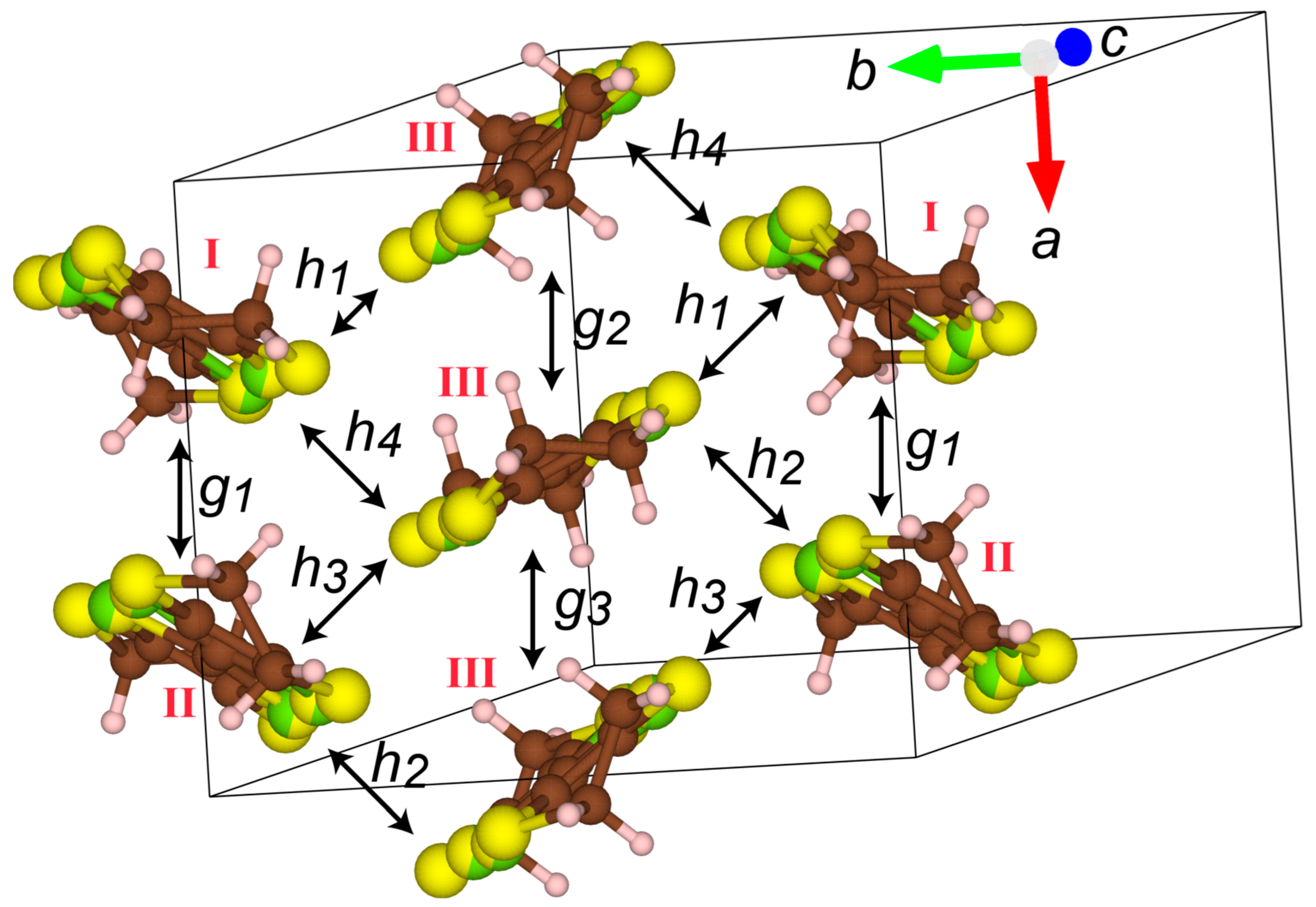
Figure 1. Crystal structure of α-STF2I3. The brown, yellow, green, blank, and violet spheres denote C, S, Se, H, and I atoms, respectively. The double-coloured (yellow and green) atoms are disordered atoms between S and Se (S: Se = 50%:50%).
Crystals 12 00346 g001
Figure 2. Two possible packing patterns of the STF molecule at a given site in α-STF2I3 (X = S or Se).
Crystals 12 00346 g002
Figure 3. Four possible packing patterns (AD) of the interacting pair of STF molecules at a given site in α-STF2I3. All four patterns should occur in the crystal with equal probability to reproduce the observed structure. Adapted from [21] and modified with permission.
Crystals 12 00346 g003
Figure 4. Intermolecular interactions between STF molecules in α-STF2I3. The unit cell contains three independent STF molecules, two halves (I and II) and one whole (III) STF molecule. All the I and II STF molecules possess an inversion centre on the central C=C bond, which means that atomic positions and electron densities are the same between Patterns 1 and 2 in Figure 2 for molecules I and II. Although molecule III does not possess an inversion centre, the atomic positions and electron densities for X in molecule III are also identical between Patterns 1 and 2.
Crystals 12 00346 g004
Figure 5. Structure of the top two bands in three-quarter filled bands based on the tight-binding model, where transfer energies tSTF were assumed as tSTF/eV = −10SSTF, and the values of SSTF were newly estimated using Equation (14) (Table 1) in this study. The tight-binding model, which is required in the band calculation using the values of tSTF, is identical to that in our previous study [21]. The obtained band structure is different from our previous study [21]. (a) Conduction and valence bands given by E1 (upper band; 0 ≤ E1 ≤ 0.51 eV) and E2 (lower band; −0.15 ≤ E2 ≤ 0 eV) as the function of wavevector k = (ka, kb). The lattice constant of the square lattice is taken as unity. The energy (eV) is measured from the chemical potential μ. The two bands contact with each other at the Dirac points (ka/π, kb/π − 1) = ± (0.21, −0.06) with the energy ED = 0.173 eV, which coincides with μ. (b) Contour plot of E1E2 with the energy range of 0 ≤ E1E2 ≤ 0.51 (eV). The Dirac points exist in the two darkest points in the orange region, which indicates 0 ≤ E1E2 ≤ 0.05 eV. The two Dirac points are close to merging at one of the TRIMs (time-reversal invariant momentum) X = (0, π) since the contour is elongated toward the X point and E1E2 is much smaller than that at other TRIMs.
Crystals 12 00346 g005
Table 1. Estimated overlap integrals (SSTF × 103/dimensionless) in α-STF2I3. HOMO-HOMO overlaps between adjacent STF radical cations.
Pairs (a)X = SeX = SX = Se or S (50%)
g1+9.0−19.7−5.35
g2−8.50−17.9−13.2
g3+2.2−11.7−4.75
h1+31.8−25.9+2.95
h2−33.7−25.3−29.5
h3−15.0−13.3−14.15
h4+6.8−8.6−0.9
(a) For the interacting STF pairs in the unit cell, see Figure 4. The extended Hückel parameters utilised in the calculations are reported in [21]. For reference, the values of S(X = Se) and S(X = S) are listed in Table 1.
Publisher’s Note: MDPI stays neutral with regard to jurisdictional claims in published maps and institutional affiliations.

