Statistical Analysis of the Distribution of the Schmid Factor in As-Built and Annealed Parts Produced by Laser Powder Bed Fusion

Abstract

This study documents a systematic analysis of the global Schmid factor for different deformation mechanisms in α′/α and β-grains in different forms of direct metal laser sintered (DMLS) Ti6Al4V(ELI) based on EBSD data. A novelty of this study is the use of these data to calculate the values of the Schmid factor and the subsequent determination of their distribution and frequency, which, when compared to the slip systems of crystal structures, helps in determining the favourable slip systems in play. Both retained β-grains and reconstructed prior β-grains were considered in this analysis. The reconstruction of the prior β-grains was executed using the Automatic Reconstruction of Parent Grain for EBSD data (ARPGE) program. The distribution of the global Schmid factor for these Ti6Al4V phases was calculated using the MATLAB-based MTEX toolbox program. This analysis of deformation modes in the α′/α-phase was based on a uniaxial load state acting on the x, y, and z axes, while only the load along the build direction (x-direction) was considered in the analysis of deformation mechanisms in the β-phase of the alloy. The results of this study showed that the DMLS build direction influenced the distribution of the global Schmid factor for the basal slip system of α′/α-grains in as-built specimens and those samples that were heat treated below the α→β transformation temperature.

1. Introduction

Metal additive manufacturing (AM) technologies, such as laser powder bed fusion (LPBF) and electron beam powder bed fusion (EPBF), are revolutionising the way products and consumer goods are manufactured. Design flexibility achieved by these technologies that are used to make parts from three-dimensional (3D) computer-aided design (CAD) model data, in a layer-by-layer fashion, as opposed to subtractive manufacturing, is now persuading scientists and engineers to create novel ideas and opportunities for industries. A variety of metals and metal alloys are being used to produce parts by LPBF, which include titanium alloys, aluminium alloys, tool steel, stainless steel, maraging steel, copper alloys, nickel alloys, and cobalt alloys [1,2,3].

The mechanical properties of metals and their alloys are greatly affected by intrinsic microstructural features, primarily grain size and crystallographic texture, as well as density, character and distribution of dislocations [4]. All of these factors are influenced by manufacturing history and post processes. Understanding the evolution of crystallographic textures during manufacturing processes is important as this could result in anisotropy of mechanical properties. The crystallographic texture of titanium alloys, such as Ti6Al4V, is greatly influenced by the manufacturing process history [5]. The Ti6Al4V alloy is a dual-phase alloy consisting of α-phase, which exhibits the low symmetrical hexagonal closed-packed (hcp) structure, and β-phase, which exists as a highly symmetrical body-centred cubic (bcc) structure [6]. Each grain in the microstructure of the alloy consists of either the α or β-phases, having crystals with similar orientations relative to a reference frame.

The laser powder bed fusion of the Ti6Al4V(extra low interstitial—ELI) alloy induces a strong fibrous texture in prior β-grains with the <001> direction aligned with the build orientation [7]. This has been associated with the continuous deposition of layers that act as heat sinks, while the laser beam provides the heat source from above. Therefore, the maximum thermal gradient during LPBF is along the build direction, which elucidates the strong fibrous texture of the prior β-grains in parts produced this way [7,8,9]. Nonetheless, the fibrous texture of the β-grains has been shown to disappear after post-process heat treatment conducted above the α→β transformation temperature [7]. The elongated prior β grains of as-built LPBF Ti6Al4V are normally filled with a non-equilibrium α′-martensitic microstructure, which transforms to equilibrium α and β -phases upon post-process heat treatment. The evolution of the prior β-phase texture has been shown to impact the texture of the resulting α′/α-phase during β→α transformation at lower temperatures through the known Burgers orientation relationship (BOR) between these two phases on the (0001)α||{110}β planes and <11$\overline{2}$0>α||<111>β directions [6,7,8,9]. During the transformation of β→α, twelve definite orientations of the α′/α- phase can result from a single prior β-grain due to this BOR, and this has been shown to weaken the texture of the α′/α-phase [9,10]. However, variant selection has been found to occur during β→α transformation, where some α′/α variants form more frequently than others due to factors such as the composition of the alloy, cooling rate, and the sizes of the prior β-grains [8,9,10].

Generally, the orientation of a crystal within a polycrystalline material is expressed by a specific rotation, which transforms the crystal fixed coordinate system into the sample-fixed coordinate system or vice versa. There are various ways of describing a rotation of two-coordinate systems with respect to each other, which can be used to analyse the crystals’ orientation in a material. These different methods are described in [11]. The three Eulerian angles $\mathit{g}$(${\phi }_1, \varphi ,{\phi }_2$) are commonly used to represent the rotation between two coordinate systems. Where ${\phi }_1$ is the first angle of rotation of the crystal coordinate system about the $z$-axis, $\varphi$ is the second angle of rotation of the new crystal coordinate system about its new x′-axis, and ${\phi }_2$ is the third angle of rotation of the new crystal coordinate system about its new $z^{\prime }$-axis. The orientation matrix obtained by composing the three Eulerian rotation angles is of the form [11]:

$$\mathit{g}\left({\phi }_1, \varphi ,{\phi }_2\right)=\left(\begin{array}{ccc}cos{\phi }_{1}cos{\phi }_2-sin{\phi }_{1}sin{\phi }_{2}cos\varphi & sin{\phi }_{1}cos{\phi }_2+sin{\phi }_{2}cos\varphi & sin{\phi }_{2}sin\varphi \\ -cos{\phi }_{1}sin{\phi }_2-sin{\phi }_{1}cos{\phi }_{2}cos\varphi & -sin{\phi }_{1}sin{\phi }_2+cos{\phi }_{1}cos{\phi }_{2}cos\varphi & cos{\phi }_{2}sin\varphi \\ sin{\phi }_{1}sin\varphi & -cos{\phi }_{1}sin\varphi & cos\varphi \end{array}\right)$$

(1)

Electron backscatter diffraction (EBSD) is a scanning electron microscope-based microstructural characterisation technique used to determine the orientation of crystals in a polycrystalline material [12]. The technique produces data with a high degree of accuracy that can be analysed to provide information such as crystallographic texture, as well as morphology and orientation of the grains, phase fraction, and local strain in a material [12,13]. The details of the orientations acquired from multiple points within a given phase in a material enable a statistical check as to whether that phase has a preferred orientation. The interpretation of crystallographic texture from an EBSD data set can be achieved through the analysis of pole figures and orientation distribution maps. However, the analysis of the poles figures and the orientation distribution maps may not necessarily identify or predict the distribution of the active deformation systems in a material under load. Rather, the Schmid law is often used to predict the activation of slip systems in a material depending on the loading axis. The law dictates that yielding in a crystal initiates when the resolved shear stress on the slip plane along the slip direction exceeds the critical resolved shear stress (CRSS) [14]. The CRSS is a material property that represents the minimum shear stress required to initiate the slip. However, the CRSS differs for different slip systems in a material and is used to quantify the ease of slip in a particular slip system. The Schmid factor ($m$) is greatly influenced by the crystallographic orientation (orientation of slip systems) of the crystals in a material and is normally expressed as [14,15].

$$m=cos\phi \cos \lambda$$

(2)

where $\phi$ denotes the angle between the loading axis and the normal to the slip plane and λ is the angle between loading axis and the slip direction. The critical resolved shear stress ($\tau$) on the other hand, is expressed as:

$$\tau ={\sigma }_{i}m$$

(3)

where ${\sigma }_i$ is the uniaxial stress acting along a given axis.

The crystallographic texture of the reconstructed prior β-grains and transformed α′/α phase in AM Ti6Al4V parts, through the analysis of pole figures and orientation maps, has recently been studied and published in the open literature [7,8,9,10,16,17]. In the present study, the statistical distribution of the Schmid factor for individual grains in as-built and annealed Ti6Al4V(ELI) samples produced by the DMLS process is analysed and presented. In this study, the $m$ values were calculated in detail for different slip systems in the α′/α-phase, including the basal, prismatic, and pyramidal slip systems, as well as for the retained and reconstructed β-grains. The results presented in this study are useful in the prediction of the active slip system that is to be used in describing the flow stress and deformation behaviour in different microstructures of LBPF Ti6Al4V(ELI).

2. Materials and Methods

2.1. Fabrication and Heat Treatment of Test Specimens

The Ti6Al4V(ELI) parts used for this study were fabricated using an EOSINT M 280 DMLS machine, a laser powder bed fusion technology from Electro Optical Systems (EOS) GmbH. The raw material was a gas-atomised spherical powder of Ti6Al4V(ELI) obtained from TLS Technik GmbH with a particle size of <40 µm (D₁₀, D₅₀, D₉₀). The specified chemical composition (wt.%) of the powder was as follows: Al 6.34, V 3.944, Fe 0.25, O 0.082, C 0.006, N 0.006, H 0.00, and the balance Ti [18]. The DMLS machine parameters set used to fabricate the specimens were as follows: laser power 175 W, laser diameter 80 µm, hatch spacing 100 µm, layer thickness 30 µm, and scanning speed 1400 mm/s.

A total of 24 cylindrical rods, each with a diameter and length of 6 mm and 80 mm, respectively, such as the one in Figure 1, were built with their longitudinal axes aligned with the z-axis of the EOSINT M 280 machine and the x-axis of the SEM used in this study. While still on the platform with support structures, some of these rods were stress relieved. Thereafter, the rods were cut away from the platform, and the support structures were removed. Each rod was then cut into 10 samples, each with a diameter and length of 6 mm.

The manufactured samples were then subdivided into five groups, designated hereinafter as samples A, B, C, D, and E. The samples group B, C, D, and E were further exposed to heat treatment in a SuperSeries™ vacuum furnace system Model SS12-24/13MX with a horizontal chamber. Samples B were just stress relieved, while samples C, D, and E were first stress relieved and subsequently heat-treated at different high temperatures to allow microstructural transformation. The stress relieving heat treatment was executed in a vacuum chamber at a temperature of 650$°$C, with a soaking time of 3 h, followed by furnace-cooling to room temperature. The heat treatment cycles for samples C, D, and E are summarised in

Table 1. The heat treatment strategies and designations of LPBF Ti6Al4V(ELI) samples.

Designation	Temperature ( $°$)	Residence Time (h)	Cooling Rate	Average Rate of Cooling
A	As-built	-	-	-
B	650	3 h	FC	-
C	800	2.5 h	CC	7.5 °C/min
D *	940 and 750	2.5 h and 2 h	CC	57.5 and 51 °C/min
E	1020	2.5 h	CC	40.5 °C/min

* Duplex annealed, FC—Furnace cooled, CC—Controlled cooling.

.

The furnace cooling rate for the B samples was obtained by switching off the furnace after the mentioned residence time and allowing the chamber to then cool to room temperature. The controlled cooling rates for samples C, D, and E shown in this table were achieved by accelerating a stream of argon gas through the furnace chamber. Further details on the selection of these heat treatment plans can be found in the authors’ previous work in [7,19].

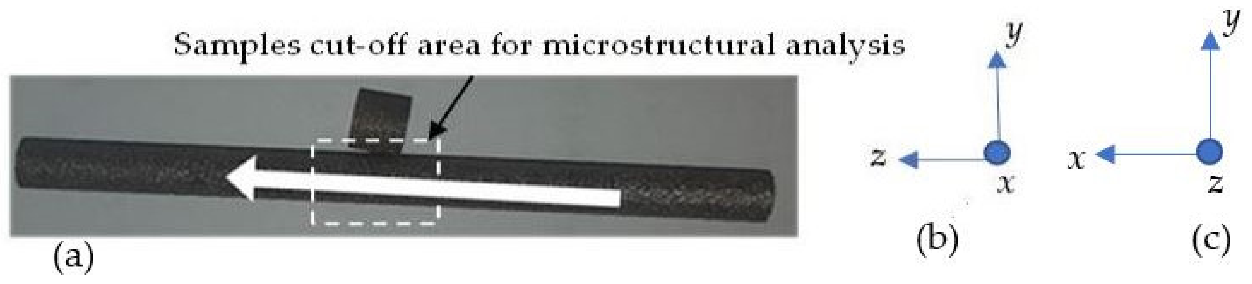
2.2. Materials Preparation

The samples to be used for microstructural analysis were cut from the middle area, along the height of the samples, as shown in Figure 1. Sample pieces, with a height of 6 mm, shown in Figure 1, were cut from the samples and then sectioned into halves across the diameter (along the build direction) using an electrical discharge machine (wire cutting). The cut surfaces were then mounted using a Citopress mounting machine, where the specimens were placed in a mounting cylinder together with Multifast resin (conductive Bakelite). Mounting was followed by grinding and chemical-mechanical polishing. The grinding was executed with SiC papers (up to 4000 grit). The chemical-mechanical polishing was executed using a mixture of colloidal silica (OP-S) and water on an MD-Chem cloth. The polished samples were thereafter cleaned under tap water before being dried using a stream of compressed air. The polished samples were not etched since, in EBSD, the grain boundaries are delineated by processing the orientation of the measured data set.

2.3. EBSD Analysis

The crystallographic texture of the samples was studied, examined, and measured using a JEOL JSM -7001F SEM that was equipped with an EBSD detector. The EBSD system was equipped with a low-light sensitive camera (CCD) and HKL Channel 5 acquisition and data manipulation software. The mounted samples were glued onto a holder pre-tilted at an angle of 70$°$ from the horizontal towards the EBSD detector to optimise both the contrast in the diffraction pattern and the fraction of electrons backscattered from the test sample. The number of grains measured is critical for quantitative texture analysis. More so, increasing the number of points at which measurements are obtained per grain also helps to better describe the grain size and shape, as well as any interior sub-grain structure, including low-angle grain boundaries. The number of points per grain is defined by the step size. Due to the small nature of grains, especially in samples A, B, and C, the scanning step size for the EBSD mapping in this study was selected to lie between 400–500 nm such that the average grain contained over 500 points. Other EBSD settings that were used for data collection in this study were as follows: a step size of 0.5 µm, a spot size of 3–5 µm, an accelerating voltage of 15 kV, a working distance of 14 mm, a magnification of X200, and a sampling grid of (X,Y) 980 × 755 µm.

The orientation distributions of various microstructures from the EBSD were acquired and processed in the HKL Channel 5 software. The post-processing of the EBSD data in the form of CFT files was conducted in MTEX, a toolbox for analysing and modelling crystallographic textures from EBSD data. The distribution of the Schmid factor for various deformation mechanisms in the α′/α and β-phases of the DMLS Ti6Al4V(ELI) that were obtained are presented and discussed in this study.

2.4. Reconstruction of Prior β-Grains

During the β→α′/α transformation, the β-phase is concealed by the dominant α-phase formed due to its relatively low volume. Therefore, it is important to establish the relationship between the small fraction of the retained β-grains and the prior β-grains in a microstructure. The orientation of the prior β-grains can be reconstructed based on the knowledge of the transformed α′/α-phase using the BOR. The computer program ARPGE developed in [20] for the reconstruction of parent grains using the orientation measured from the daughter variants in the EBSD scans was used in this study.

Steps were taken to identify the α′/α belonging to the same mother-β-grain by considering the specific misorientation angles and axes between the adjoining grains. Further details of the reconstruction process used in this study can be found in [7]. The reconstructed β-grains were then exported to a file compatible with MTEX (.cft) for further analysis. The distribution of the Schmid factor for the active slip systems in retained β-grains and reconstructed prior β-grains are reported here.

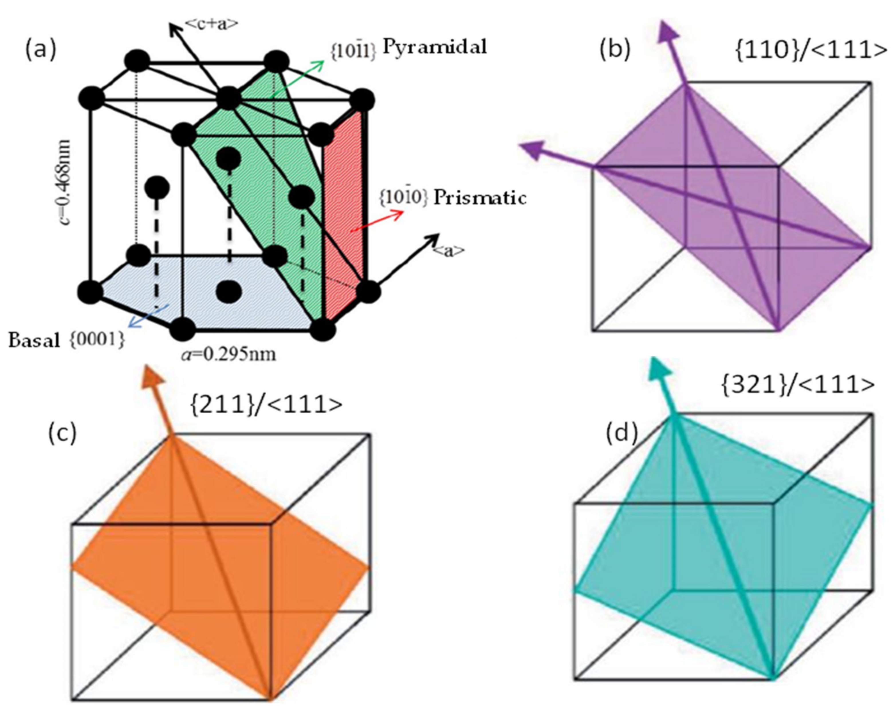
2.5. Calculation of Schmid Factor for Different Slip Systems in the α and β-Phases Using MTEX Toolbox

Euler angles, as previously mentioned in Section 1, are normally used to present the orientation of individual crystals/grains with reference to a fixed coordinate system. On the other hand, the rotation matrix ($\mathit{g}$) shown in Equation 1 is used to transform the crystal coordinate system into a sample coordinate system. The MTEX-toolbox program was used to calculate the Schmid factor for all of the slip systems for a given orientation. The input to the program was the EBSD data of the three Euler angles for each grain in the material.

The slip system in each crystal consists of the slip plane and the slip direction, which are expressed using Miller indices as ($\mathit{h}\mathit{k}\mathit{l}$) and ($\mathit{u}\mathit{v}\mathit{w}$), respectively. Thus, the transformation of the slip system from the crystal coordinate system to the sample coordinate system is given as:

$$n=\mathit{g}•\left(\begin{array}{c}\mathit{h}\\ \mathit{k}\\ \mathit{l}\end{array}\right) \mathrm{and} b=\mathit{g}•\left(\begin{array}{c}\mathit{u}\\ \mathit{v}\\ \mathit{w}\end{array}\right)$$

(4)

where symbols $n$ and $b$ denote the transformed slip plane normal and the slip direction of a given slip system, corresponding to the sample coordinate system. The global stress state acting on the sample was assumed to be uniaxial expressed as, ${\sigma }_i$. The schematic diagram in Figure 2 shows the loading axis of the samples in reference to the SEM coordinate system and the corresponding second rank stress tensors acting along each of the axes. It should be noted that the x-axis of the SEM used for this study corresponded with the build orientation (z-axis) during the DMLS process, as shown in Figure 1.

Thus, the global Schmid factor $m$ for each slip system in an individual grain was calculated by resolving the stress in the slip direction of a given slip plane as:

$$m=b•n•{\sigma }_i$$

(5)

It is important to note that there are three different slip systems in the α′/α-phase of titanium, viz. basal, prismatic, and pyramidal slip systems, as shown in Figure 3a. Each of these slip planes has a preferred slip direction(s). These slip systems and the number of their variants that were analysed in this study are shown in

Table 2. The number of α′/α-titanium slip systems analysed in this study.

Slips System	Slip Plane	Slip Direction (<a>)	Number of Variants
Basal	<0001>	($11\overline{2}0$)	3
Prismatic	{$10\overline{1}0$}	($11\overline{2}0$)	6
Pyramidal	{$10\overline{1}1$}	($11\overline{2}0$)	12

.

It is worth mentioning that glide along the pyramidal plane can also occur by the movement of <c+a> type dislocations. However, the large Burgers vector of <c+a> type dislocations on pyramidal planes result in high values of the CRSS on these planes [21]. Thus, the probability of grains deforming by <c+a> dislocations is very low in Ti6Al4V alloy [22]. Therefore, the {$10\overline{1}1$}|<$11\overline{2}3$> slip system and its variants were not considered in this study.

The slip planes for bcc titanium are normally taken to be {110}, {211}, and {321}, with the slip direction being <111> for all planes, as shown in Figure 3b–d. Each of these slip systems has 32 invariants.

3. Results and Discussion

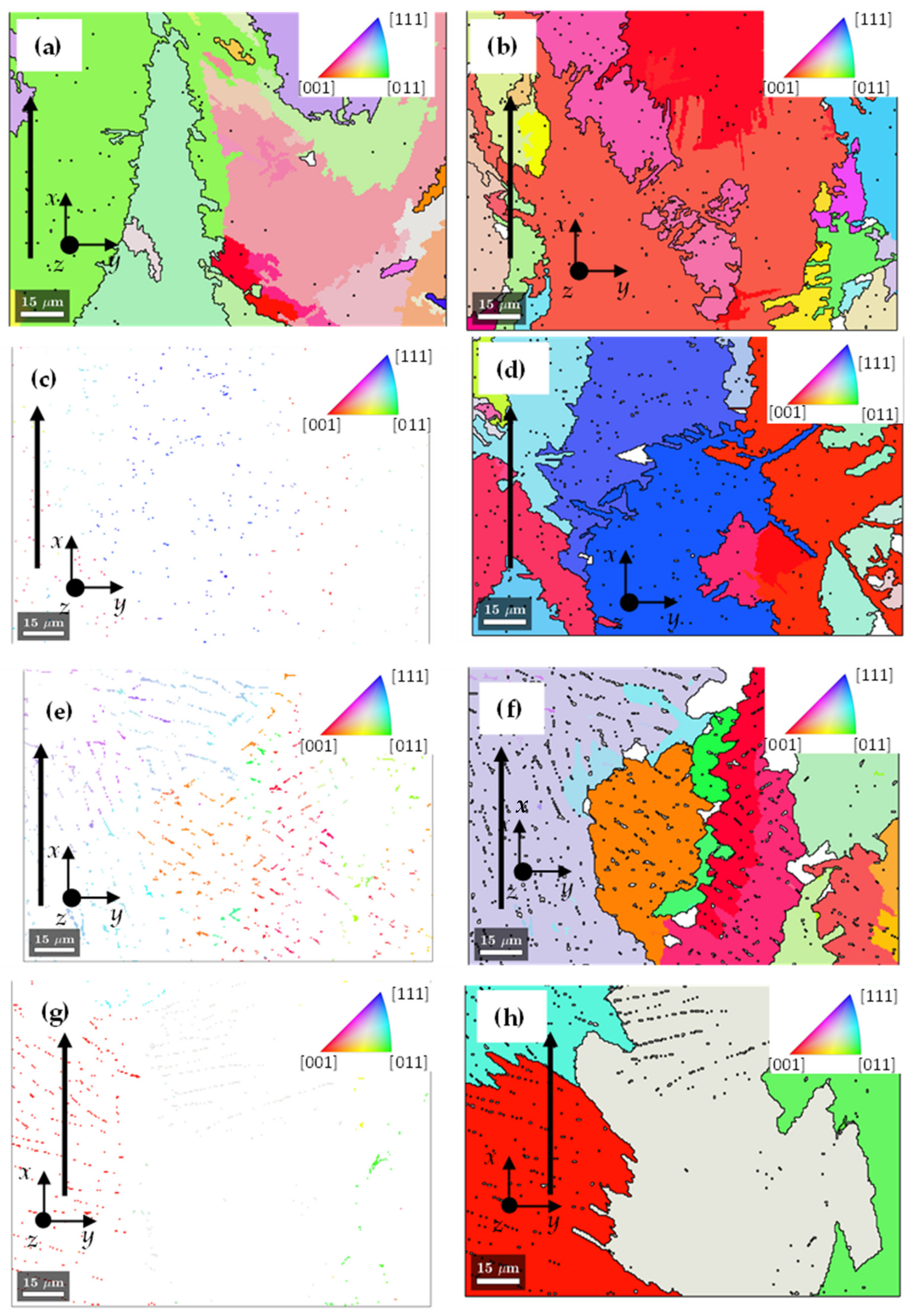
3.1. Orientation Distribution and Volume Fraction of Phases

The Ti6Al4V alloy is generally composed of crystalline grains of either an α or β- phase, with each grain having a crystal structure with a uniform crystalline orientation relative to a reference frame. The proportion of either of these phases is dependent on the processing history and the post-process heat treatment adopted. For the different forms of DMLS Ti6Al4V(ELI) in Table 1, the volume fractions of α and β-phases were studied using the EBSD and XRD methods. A summary of the results from these analyses, as reported in [7,19], are presented in

Table 3. The percentage volume fraction of α and β-phases as estimated by EBSD and XRD [7,19].

Method of Analysis	EBSD		XRD
Type of phase	α′/α	β	α′/α	β
Samples A	100%	0	100%	0
Samples B	100%	0	100%	0
Samples C	98.9%	1.1%	96.4%	3.6%
Samples D	94.9%	5.1%	93,6%	6.4%
Samples E	97.3%	2.7%	93.4%	6.6%

.

The different percentage fractions of the α- and β-phases recorded using the EBSD and XRD methods for the same material were ascribed to the inhomogeneous distribution of the β-phase in these microstructures. The EBSD results were based on a micro-grid area of 980 µm × 735 µm, while the XRD scans were conducted on the bulk surface of the samples. Thus, the results from XRD were taken to be a better representation of the bulk microstructure of each group of samples. For detailed analyses of the microstructures obtained after the heat treatments described in Table 1, the reader is referred to the authors’ previous work published in [7,19]. Figure 4 and Figure 5 show the orientation distribution of α′/α, retained β-grains and reconstructed prior-β grains in various forms of DMLS Ti6Al4V(ELI), respectively.

The orientation distributions of the grains in polycrystalline materials are usually dependent on processing history. The alignments of these crystals cause the material to have either a preferred or random crystallographic texture. As shown in the micrographs in Figure 4 and Figure 5, the z-axis of the SEM was orthogonal to the sample surfaces, which was the direction of the EBSD scans. As noted earlier in this paper, the x-axis of the SEM was aligned to the build direction of the samples during the DMLS process. Due to the high thermal gradient along the build direction associated with the DMLS process, the Ti6Al4V(ELI) parts manifested a preferential <100> direction texture for the prior β-grains [8,9]. This is clearly shown in Figure 4a–c and Figure 5a,b,d,f, where the prior β grains are shown to be elongated along the build direction. A preferred texture is expected to result in anisotropy of mechanical properties. However, DMLS parts have been shown to possess relatively isotropic mechanical properties [23,24], suggesting that the preferred prior β-texture does not cause the anisotropy of the mechanical properties in this case.

The crystallographic texture of the α′/α laths are illustrated by the Euler angles for all of the samples shown in Figure 4. The inverse pole figure’s key in Figure 4f shows the colour codes related to the given orientations, such that the family of planes $\left\{1\overline{1}00\right\}$, $\left\{0002\right\}$, and $\left\{11\overline{2}0\right\}$ are represented by the colours blue, red, and green, respectively. The specific orientations are observed parallel to the XY-surface. As β-grains transform to α′/α-grains during the cooling process and following the well-known BOR between these two phases [25], 12 variants of the latter can be precipitated from each of the former grains. The transformation of the β-phase to the 12 variants of the α′/α-phase during cooling has been shown to give rise to the random texture of the material [7,9], thus raising the possibility of the anisotropy of the mechanical properties. It is rare that all the 12 variants of the α′/α-phase occur with equal probability, and some α′/α lath orientations tend to occur more frequently than others within the same prior β-grain, as shown in Figure 4a–d. This preference for certain variants to occur more than others has been attributed to variant selection during the β→α transformation [8,22]. For a detailed analysis of the variant selection in the DMLS Ti6Al4V(ELI) parts, using pole figures, the reader is referred to the authors’ previous work in Muiruri et al. [7].

The samples heat treated above the α→β transformation temperature are characterised by decomposed prior β-grains, which leads to the formation of equiaxed and semi- equiaxed grains as shown in Figure 4e and Figure 5h. The crystallographic texture of the retained β grains in Figure 5c,e,g is seen to be the same as that of the reconstructed β-grains in Figure 5d,f,h. This is further confirmed by the (100) plane contour pole figures of the reconstructed prior β grains and retained β-phase in the samples C, D and E shown in Figure 6. In this figure the poles of the reconstructed prior β-grains are seen to coincide with those of the retained β-grains.

The analysis of these pole figures shows that the (100) poles are mainly concentrated approximately along the $x$-build direction in both cases of the retained β-grains and the reconstructed prior-β grains in samples C and D. This confirms that the retained β-grains in Ti6Al4V(ELI) formed during the DMLS cooling process possess a typical fibrous texture. Due to the decomposition of the prior β-grains after heat treatment above the α→β transformation temperature in the E samples, the concentration of the poles along the $x$-direction disappeared, as seen in Figure 6. The crystallographic orientations of some of the grains in the E samples seem to have rotated at angles of 37° to the build direction in both cases of reconstructed and retained β-grains (circled in Figure 6). Such a rotation could influence the Schmid factor of such grains and is investigated in Section 3.3 of this paper.

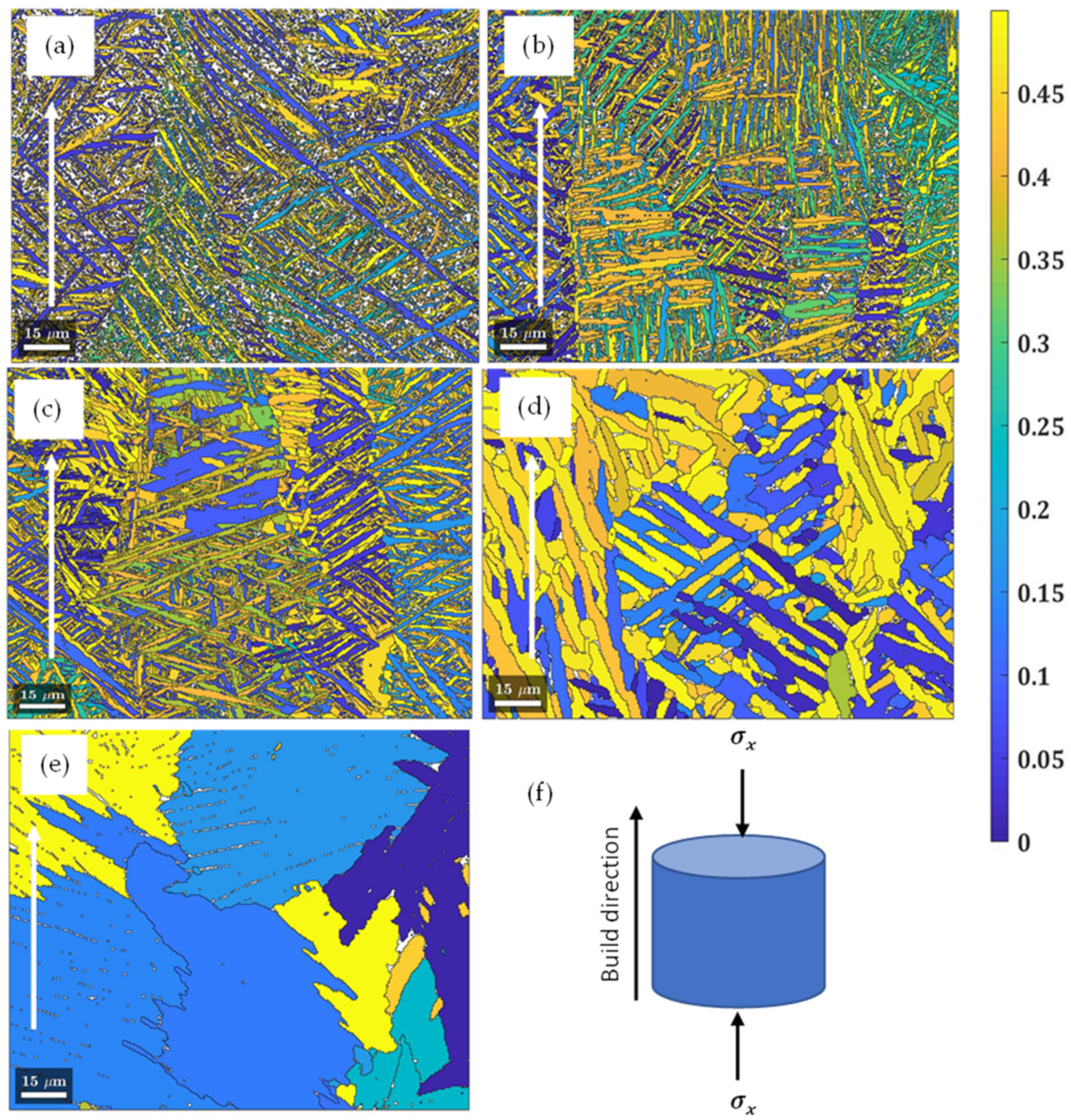
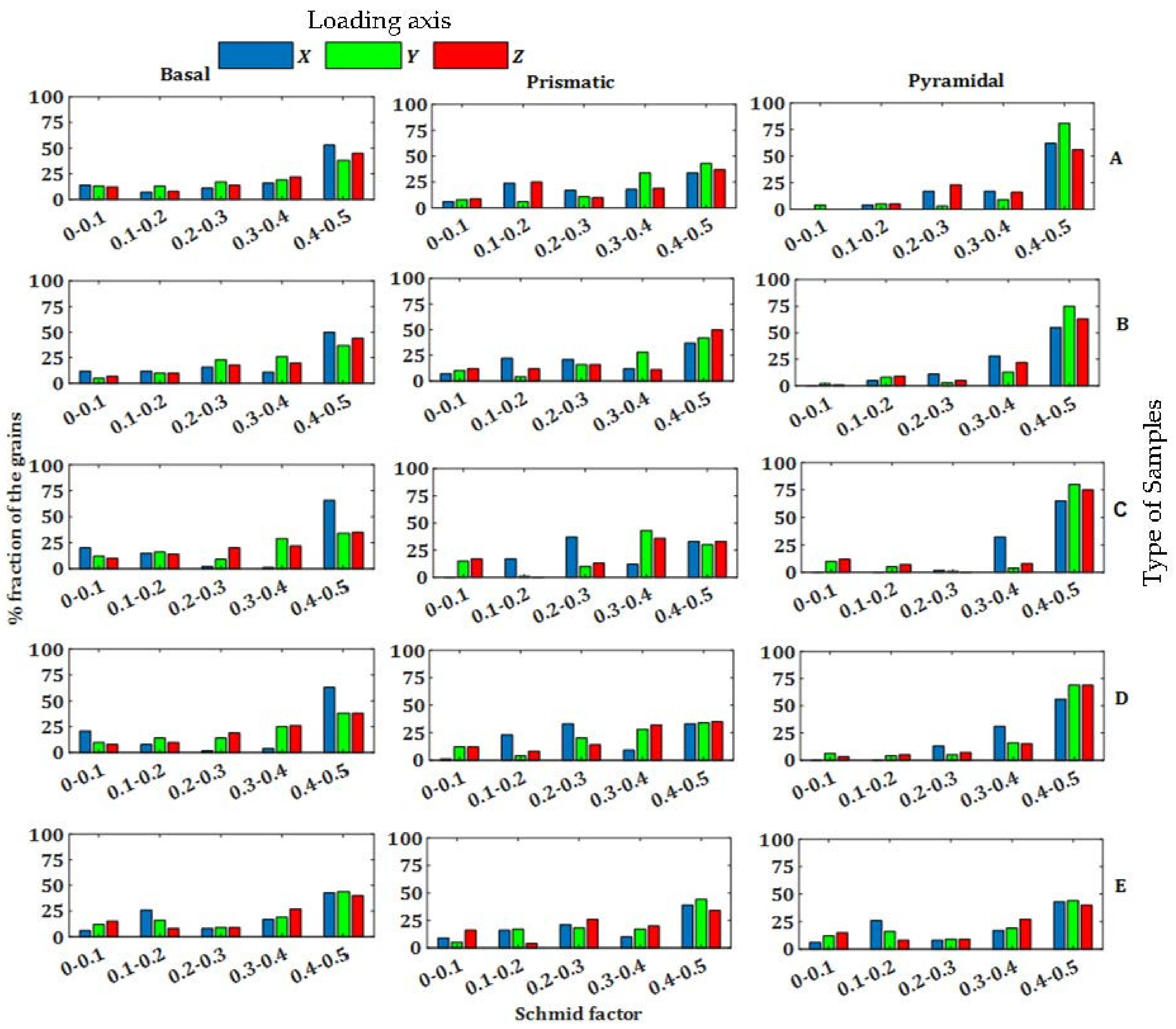
3.2. Schmid Factor Distribution of α′/α-Phase in Various Microstructures of DMLS Ti6Al4V(ELI)

Figure 7 shows classical calculated values and distribution of the global Schmid factor for the basal slip system of the α′/α -grains in different forms of DMLS Ti6Al4V(ELI). The values in this figure were obtained based on the uniaxial load acting along the build direction (x-axis) shown in Figure 1. The maps of the global Schmid factor are coloured by codifying the obtained values of the global Schmid factor and then transforming them into the red, green, and blue (RGB) colour space for each pixel (Euler angles). The legend on the right side of the figure indicates the range of values for $m$, from 0 to 0.5. A Schmid factor $m$ = 0 indicates that the slip plane normal or the slip direction is parallel or orthonormal to the loading direction, respectively. Thus, according to Equations (2) and (3), there is no shear stress acting on such a slip system. Such crystals will slip on different slip systems in which the Schmid factor for the applied load is higher than zero. As the angle between the slip plane normal or the slip direction and the loading axis increases or decreases from 0° and 90°, respectively, the $m$ value increases with an attendant increase in the ease of slip on the planes and the directions of closest packing. The Schmid factor is at a maximum ($m=0.5$) when the angle between the loading axis and slip plane normal and the slip direction is 45°, which is commonly referred to as the angle of maximum shear.

As shown in the micrographs in Figure 7, the calculated values of the global Schmid factor for the basal slip system of the α′/α–grains in various microstructures of DMLS Ti6Al4V(ELI) are distributed across the full range of values for the factor. While the micrographs in Figure 7 show a section of sampled area, statistical analysis of the distribution of the global Schmid factor in the α′/α-grains for the entire sampling grid area of 980 × 755 µm for the samples is summarised in Figure 8. In this analysis, the values of the global Schmid factor were obtained for each of the three-stress tensors (${\sigma }_x$, $0$, $0$), ($0$, ${\sigma }_y$, $0$) and ($0$, $0$, ${\sigma }_z$) shown in Figure 2, acting on the samples, one at a time.

The plots in Figure 8 are for the frequency of orientation of the grains as defined by the determined global Schmid factor. As seen in this figure, more than 50% of the grains for samples A, B, C, and D have their global Schmid factor values for the basal slip system in the range of 0.4–0.5 for the load applied along the build orientation (x-axis). This suggests that more than half of the grains in the four different forms of the alloy have their $\left\{0001\right\}$_α′/α planes oriented at an angle between 27 ° and 63 ° to the build direction, thus the high values of the global Schmid factor along this direction.

A typical example of the distribution of the global Schmid factor for the basal slip system in the D samples, with hexagonal closed-packed (hcp) crystal structures overlaid on the α-laths, is shown in Figure 9. In this figure, the α-laths with low values of the global Schmid factor (shown in blue colour) have their $\left\{0001\right\}$_α′/α planes or direction of Burgers vector almost parallel or normal to the load axis, respectively. On the other hand, α-laths with higher values of the global Schmid factor have their $\left\{0001\right\}$_α′/α-planes or the Burgers vector near 45° to the load axis.

It is not surprising how large the number of laths in samples A, B, C, and D that have higher values of the global Schmid factor (>0.4) are, considering the relationship of the Burgers orientation between α and β-phases during transformation and the strong fibrous texture in the <100> direction of the prior β-grains. In Figure 9b,c, two orientations of the $\left\{110\right\}$-planes (slip planes in bcc structure) are shown, where in Figure 9b, the slip plane is at 45 ° and in Figure 9c it is parallel to the direction <100>.

Among the six slip planes in a single bcc structure, four of them are oriented at an angle of 45° to the <100> direction, while the remaining two are normally parallel to the <100> direction. Therefore, due to the strong fibrous texture in the <100> direction of prior-β grains along the build direction, there is a likelihood that approximately 67% of $\left\{110\right\} \beta$-planes transform to $\left\{0001\right\} {\alpha }^{\prime }/\alpha$ oriented at angles close to 45 ° to the build direction. There are also more grains with global Schmid factors in the range of 0.4–0.5 in samples A, B, C, and D for the load acting in the $x$-direction than that along the $y$ and $z$-direction for the basal slip system. The preceding discussion suggests that a large percentage of the α′/α-grains in DMLS Ti6Al4V(ELI) will have higher values of global Schmid factor for the basal slip system for a load applied along the build direction, as seen in Figure 8.

The influence of the build direction on the global Schmid factor of the α′/α-basal slip system is slightly reduced in the E samples, with only 43% of the grains having an $m$-value above 0.4, as seen in Figure 8. Furthermore, the percentage of the grains with an $m$-value above 0.4 for the basal slip system in the E samples for the load acting in either one of the three mutually orthogonal x, y, and z directions is approximately the same (43, 44, and 40%, respectively). The possible reason for this observation is the decomposition of columnar prior β-grains after the post-process heat treatment above the α→β-transformation temperature, as reported in [7].

The statistical analysis in Figure 8 shows that 33% to 50% of the grains have their values of global Schmid factor for the prismatic slip system being $\ge$0.4 for the loads applied along either of the three mutually perpendicular axes for all the five different forms of DMLS Ti6Al4V(ELI). Clearly, the build orientation does not seem to influence the calculated values of the global Schmid factor of the prismatic slip system in either form of the alloy. A similar observation applies to the pyramidal slip system in all five groups of samples. This is possibly because there is no Burgers orientation relationship between the α′/α-prismatic and pyramidal slip planes and the prior β-grain slip planes. There is a higher number of α′/α grains, with the global Schmid factor of the pyramidal slip system being $\ge$0.4, compared to the basal and prismatic slip systems in samples A, B, C, and D, especially for the uniaxial load acting along the y- and x-axes.

It is important to note that the ease of slip on a given slip system is quantified by the CRSS, and different slip systems have different values of CRSS. Different values of CRSS for the same slip systems of the Ti6Al4V alloy have been reported, and there seems to be a lack of consensus on the actual value in the literature [26,27,28,29,30,31]. Hongmei et al. [27] attributed this uncertainty in the value of CRSS to the difficulty with its measurement, especially for non-cubic metallic structures. Some of the reported values of CRSS at room temperature for different slip systems of Ti6Al4V polycrystals are shown in

Table 4. The CRSS for different slip systems in α′/α-grains at room temperature.

Slip System	Basal<α>	Ref	Prismatic<α>	Ref	Pyramidal<α>	Ref	Pyramidal<c+α>	Ref
	388 MPa	[26]	373 MPa	[26]	401 MPa	[27]	631 MPa	[27]
	345 MPa	[27]	355 MPa	[27]	395 MPa	[31]	612 MPa	[27]
	325 MPa	[27]	342 MPa	[28]	404 MPa	[31]	640 MPa	[29]
	373 MPa	[28]	388 MPa	[29]
	400 MPa	[29]	380 MPa	[30]
	404 MPa	[30]	392 MPa	[31]

, and the ranges of values in this table are presented in Figure 10.

As seen in Table 4 and Figure 10, at room temperature, there are variations in the differences in the values of CRSS for all four slip systems. This difference is comparatively smaller between the basal<α>, prismatic<α> and pyramidal<α> slip systems than between them and the pyramidal slip system with <c+α> Burgers vector.

The uniaxial stress required to initiate slip against the global Schmid factor is presented in Figure 11 using the upper and lower values of CRSS for each slip system given in Table 4 and presented in Figure 10. As expected, the uniaxial stress required to initiate slip decreases as the Schmid factor increases. The ranking sequence for the different deformation mechanisms in terms of uniaxial stress required to initiate slip from low to high is seen in Figure 10 and Figure 11 to be basal<α>, prismatic<α>, pyramidal<α> and pyramidal<c+α>, with higher differences for the lower than upper values for the first three slip system.

Various α′/α grains in a material will obviously require different values of uniaxial stress to initiate glide due to their different orientations. This suggests that the global Schmid factor distribution shown in Figure 8 plays a pivotal role in determining the percentage of grains in a material that will deform in a given slip system for a given applied stress.

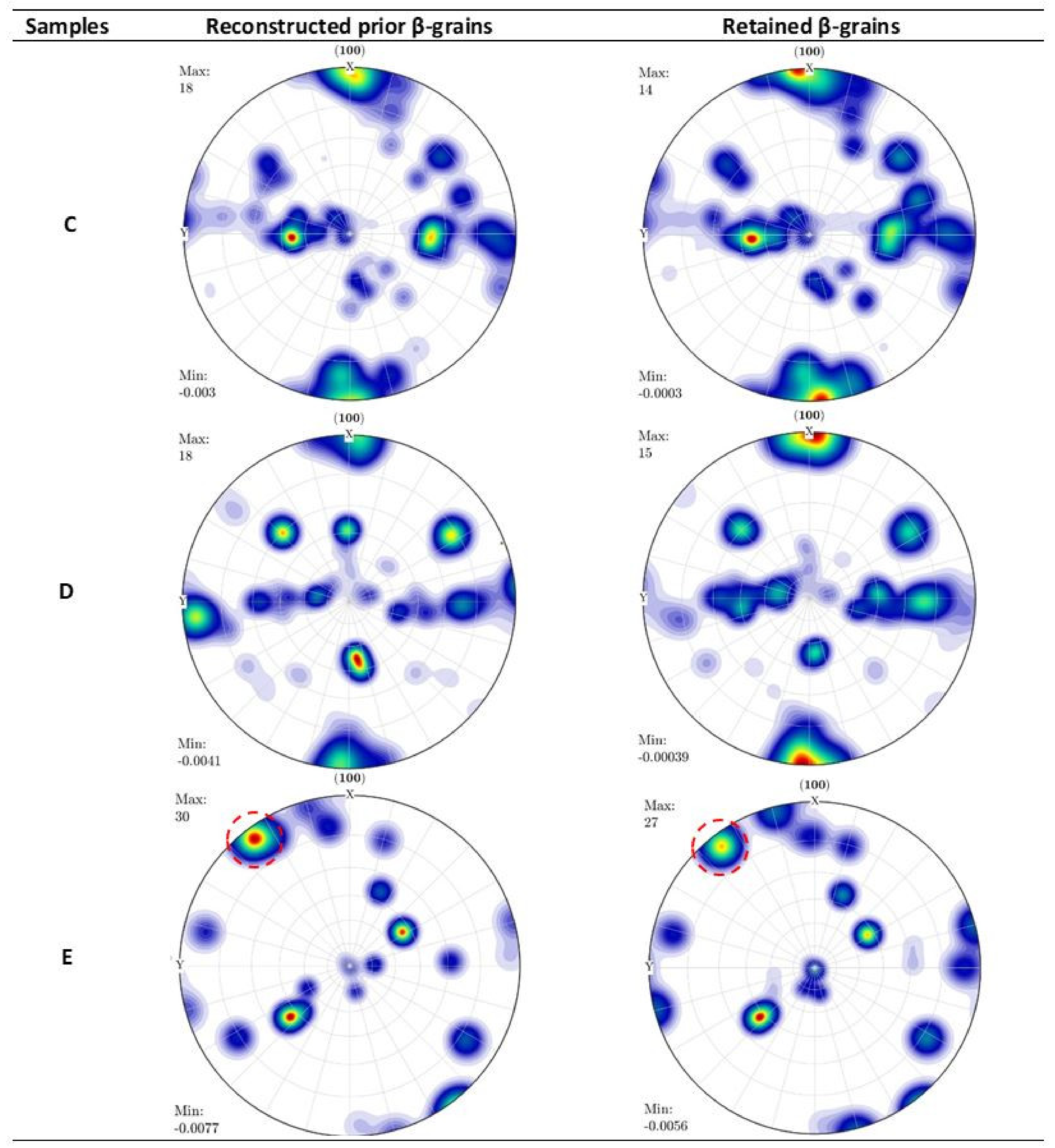
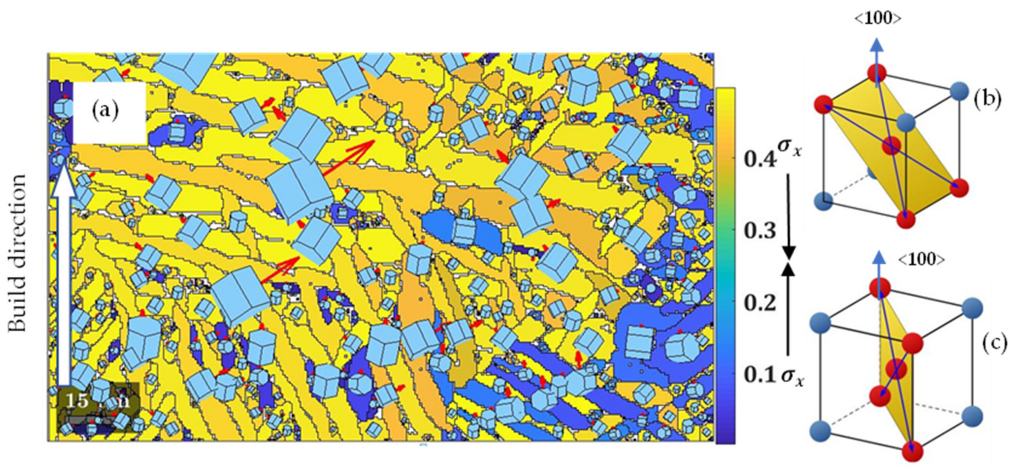
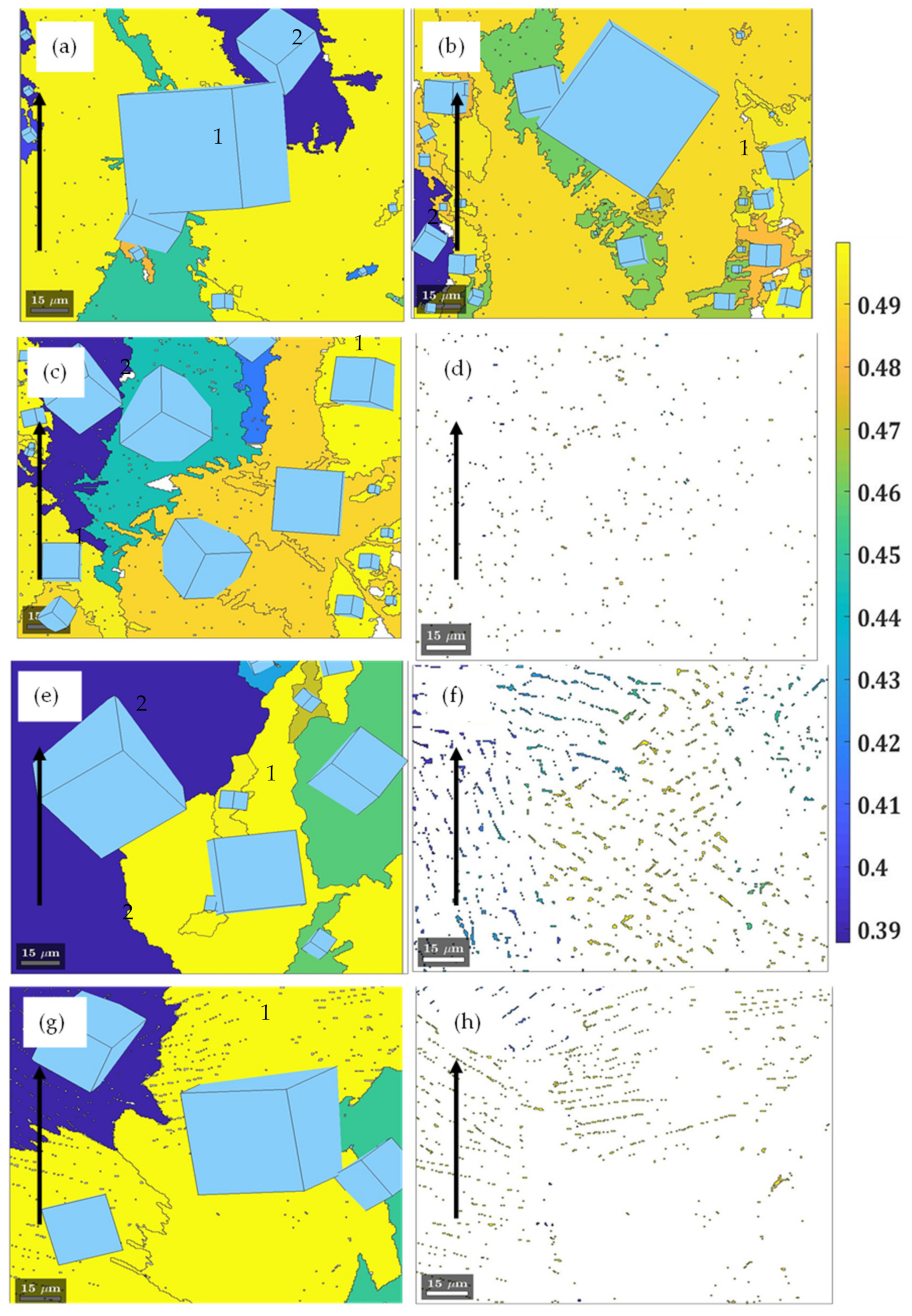
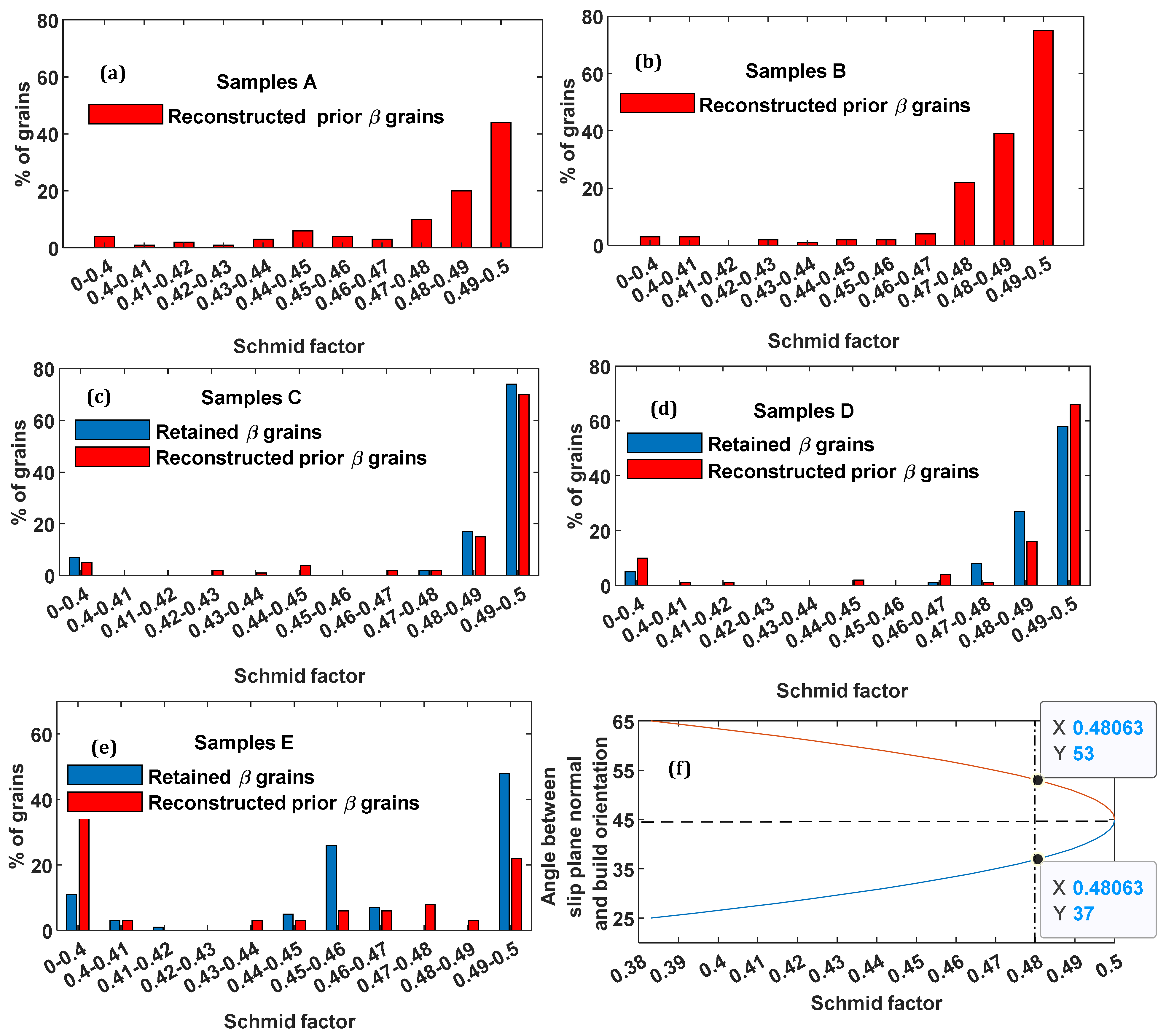
3.3. Schmid Factor Distribution of Retained β-Grains and Reconstructed Prior β-Grains in Various Microstructures of DMLS Ti6Al4V(ELI)

A typical distribution of the global Schmid factor for the reconstructed prior-β grains in samples A, B, C, D, and E and retained β-grains in samples C, D, and E is shown in Figure 12. The bcc structure is overlaid on each of the prior β-grain to demonstrate the orientation of the crystal structures in those grains with reference to the build direction. The statistical analysis of this distribution of the global Schmid factor for the EBSD scanned area is summarized in Figure 13. It is important to note that, similar to the previous section, the load axis was along the build direction (x-axis) shown in Figure 1.

It is evident in Figure 12 and Figure 13 that over 90% of the grains (either reconstructed prior-β grains or retained β-grains) in the samples of A, B, C, and D have values of the global Schmid factor that are >0.4. In fact, over 60% of the grains in these four different groups of samples have global Schmid factors between 0.48 to 0.5. This suggests that most of the β grains in these samples have their slip planes at angles in the range of 37° and 53° to the build direction, as shown in Figure 12f. If the bcc crystal structures in prior β-grains are perfectly stacked along the build direction, four of the six slip planes shown in Figure 9b would be at an angle of 45° to the build orientation, thus having the maximum value of the global Schmid factor of 0.5. However, as seen in Figure 12, the prior-β grains with the highest value of global Schmid factor (marked 1 in the figure) have a small angle of orientation ($\le$6°) to the build direction. As the angle of orientation between the cubic structure and the build direction increases, as is the case for the grains marked 2 in Figure 12, the values of the global Schmid factor decrease. The angle of orientation between the build direction and bcc crystal structures in grains marked 2 in Figure 12 is estimated to lie between 18° and 20°, thus giving $m$-values between 0.39 and 0.4.

The distribution of the global Schmid factor in the E samples show an inconsistency when compared with those of samples A to D, as seen in Figure 12f. For instance, about 36% of the reconstructed prior β-grains in the E samples have values of global Schmid factor < 0.4, while only 22% of these grains have their value in the range of 0.49–0.5. Samples A to D show percentages that increase towards the higher values of the global Schmid factor. Even though a large percentage (48%) of the retained β-grains showed values of the global Schmid factor at the highest end, about 36 % of the grains have their value in the range of 0.45–0.46. Samples C and D show very little occurrence of the retained β-grains in the mid-range values of the global Schmid factor and a gradual increase towards the higher values. The inconsistency shown in the samples of E can be ascribed to the decomposition of the prior β-grains upon heat treatment, leading to some realignment of the bcc crystal structures, as shown in the pole figures in Figure 6.

4. Conclusions

The global Schmid factor of the three slip systems (basal<α>, prismatic<α> and pyramidal<α>) for the α′/α-phase and slip systems in the β-phase were systematically calculated in five different forms of DMLS Ti6Al4V (ELI). The following conclusions were deduced from this analysis:

• The crystallographic orientation of the retained β-grains and that of reconstructed prior β-grains was found to be the same and was further confirmed by the pole figures of these grains.
• The determined values of the global Schmid factor for the α′/α-phase of DMLS Ti6Al4V(ELI) were distributed across the full range of values (0–0.5).
• More than 50% of the grains in samples A, B, C, and D had their global Schmid factor for the basal slip system at the highest range of 0.4–0.5 for a load acting along the build direction.
• The influence of the build direction on the global Schmid factor of the α′/α -basal slip system diminished in the E samples that were heat treated above the α→β transformation temperature. The percentage of grains with $m\ge$ 0.4 for this type of slip system was approximately the same for the load applied in any one of the three mutually orthogonal x-, y-, and z-directions.
• The build direction did not seem to influence the distribution of the global Schmid factors for the prismatic and pyramidal slip systems.
• There was a higher number of α′/α grains with the global Schmid factor in the pyramidal slip system $\ge$ 0.4, compared to the basal and prismatic slip systems in samples A, B, C, and D, especially for the uniaxial load acting along the y- and z-axes.
• Over 90% of the retained β-grains and reconstructed prior β-grains in samples A, B, C, and D had values of the global Schmid factor > 0.4 for loads acting along the build direction. Furthermore, over 60% of the grains in these four different groups of samples had their global Schmid factors in the highest range of 0.48 to 0.5.
• Only 22% and 48% of the reconstructed prior β-grains and retained β-grains, respectively, had their global Schmid factors in the highest range of 0.48–0.5.

Future research should aim at performing the slip trace analysis on various microstructures of DMLS Ti6Al4V(ELI) deformed at predetermined levels of strain.

References

1. Dutta, B.; Froes, F.H. The additive manufacturing (AM) of titanium alloys. In Titanium Powder Metallurgy; Elsevier Inc.: Victoria, Austria, 2015; pp. 447–468. [Google Scholar] [CrossRef]
2. Senthamarai, C.; Chandra, S.; Krishnan, P.; Pravin, S. A review on additive manufacturing of AA2024 and AA6061 alloys using powder bed fusion. IOP Conf. Ser. Mater. Sci. Eng. 2020, 988, 012002. [Google Scholar] [CrossRef]
3. Haghdadi, N.; Laleh, M.; Moyle, M.; Primig, S. Additive manufacturing of steels: A review of achievements and challenges. J. Mater. Sci. 2021, 56, 64–107. [Google Scholar] [CrossRef]
4. Dieter, E.G. Mechanical Metallurgy, 3rd ed.; Materials Science and Engineering Series; McGraw-Hill: New York, NY, USA, 1986; pp. 255–258. [Google Scholar]
5. Kocks, U.F.; Tomé, C.N.; Wenk, H.R. Texture and Anisotropy: Preferred Orientations in Polycrystals and Their Effect on Materials Properties; Cambridge University Press: New York, NY, USA, 1998; pp. 10–44. [Google Scholar]
6. Lütjering, G.; Williams, J.C. Alpha + Beta Alloys. In Titanium; Engineering Materials and Processes; Springer: Berlin/Heidelberg, Germany, 2003; pp. 177–232. [Google Scholar] [CrossRef]
7. Muiruri, A.; Maina, M.; du Preez, W. Crystallographic Texture Analysis of As Built and Heat-Treated Ti6Al4V (ELI) Produced by Direct Metal Laser Sintering. Crystals 2020, 10, 699. [Google Scholar] [CrossRef]
8. Obasi, G.C.; Bircosa, S.; Quinta, F.J.; Preuss, M. Effect of β grain growth on variant selection and texture memory effect during α→β→α phase transformation in Ti6Al4V. Acta Mater. 2012, 60, 1048–1058. [Google Scholar] [CrossRef]
9. Simonelli, M.; Tse, Y.Y.; Tucks, C. The formation of α+β microstructure in as-fabricated selective laser melting of Ti6Al4V. J. Mater. Res. 2014, 29, 2028–2035. [Google Scholar] [CrossRef] [Green Version]
10. Beladi, H.; Chao, Q.; Gregory, S. Variant selection and intervariant crystallographic planes distribution in martensite in a Ti6Al4V alloy. Acta Mater. 2014, 80, 478–489. [Google Scholar] [CrossRef]
11. Bunge, H.J. Texture Analysis in Materials Science; Butterworth & Co.: Oxford, UK, 1982; pp. 3–8. [Google Scholar]
12. Britton, T.B.; Jiang, J.; Guo, Y.; Clemente, V.A.; Wallies, D.; Hansen, L.N.; Wainkelmann, A.; Wilkinson, A.J. Tutorial: Crystal orientations and EBSD—Or which way is up? Mater. Charact. 2016, 117, 113–126. [Google Scholar] [CrossRef] [Green Version]
13. Valerie, R. Electron backscatter diffraction: Strategies for reliable data acquisition and processing. Mater. Charact. 2009, 60, 913–922. [Google Scholar] [CrossRef]
14. Callister, W.D. Material Science and Engineering: An Introduction, 7th ed.; John Wiley & Sons, Inc.: New York, NY, USA, 2007; p. 182. [Google Scholar]
15. Bertrand, E.; Castany, P.; Péron, I.; Gloriant, T. Twinning system selection in a metastable β-titanium alloy by Schmid factor analysis. Scr. Mater. 2011, 64, 1110–1113. [Google Scholar] [CrossRef] [Green Version]
16. Charlotte, F.; Michotte, S.; Rigo, O.; Germain, L.; Godet, S. Electron beam melted Ti6Al4V: Microstructure, texture and mechanical behaviour of the as built and heat-treated material. Mater. Sci. Eng. A 2016, 652, 105–119. [Google Scholar] [CrossRef]
17. Chandramohan, P. Laser additive manufactured Ti6Al4V alloy: Texture analysis. Mater. Chem. Phys. 2019, 226, 272–278. [Google Scholar] [CrossRef]
18. Titanium for Additive Manufacturing (Data Sheet for Standard Sizes and Chemistry). Available online: https://www.tls-technik.de/en/titanium-powder.html (accessed on 8 December 2021).
19. Muiruri, A.; Maina, M.; du Preez, W. Evaluation of Dislocation Densities in Various Microstructures of Additively Manufactured Ti6Al4V (ELI) by the Method of X-ray Diffraction. Materials 2020, 13, 5355. [Google Scholar] [CrossRef] [PubMed]
20. Cayron, C. ARPGE: A computer program to automatically reconstruct the parent grains from electron backscatter diffraction data. J. Appl. Crystallogr. 2007, 40, 1183–1188. [Google Scholar] [CrossRef] [PubMed] [Green Version]
21. Singh, G.; Sen, I.; Gopinath, K.; Ramamurty, U. Influence of minor addition of boron on tensile and fatigue properties of wrought Ti6Al4V alloys. Mater. Sci. Eng. A 2012, 540, 142–151. [Google Scholar] [CrossRef]
22. Dragomir, I.C.; Ungar, T. Contrast factors of dislocations in the hexagonal crystal system. J. Appl. Crystallogr. 2002, 35, 556–564. [Google Scholar] [CrossRef]
23. Moletsane, G.; Krakhamalev, P.; Du Plessis, A.; Yadroitsava, I.; Yadroitsev, I. Kazantseva, I. Tensile properties and microstructure of direct metal laser sintered Ti6Al4V(ELI) alloy. SAJIE 2016, 27, 110–121. [Google Scholar] [CrossRef] [Green Version]
24. Malefane, L.B.; Du Preez, W.B.; Maringa, M. High cycle fatigue properties of as-built Ti6Al4V(ELI) produced by direct metal laser sintering. SAJIE 2017, 28, 188–199. [Google Scholar] [CrossRef] [Green Version]
25. Burgers, W. On the process of transition of the cubic-body- centered modification into the hexagonal- close- packed modification of zirconium. Physica 1934, 1, 561–586. [Google Scholar] [CrossRef]
26. Bridier, F.; Villechaise, P.; Mendez, J. Analysis of the different slip systems activated by tension in a α/β titanium in relation with local crystallographic orientation. Acta Mater. 2004, 53, 555–567. [Google Scholar] [CrossRef]
27. Hongmei, L. Analysis of the Deformation Behavior of the Hexagonal Close-Packed Alpha Phase in Titanium and Titanium Alloys. Ph.D. Thesis, Michigan State University, East Lansing, MI, USA, 2013. [Google Scholar]
28. Hémery, S.; Villechaise, P. In situ EBSD investigation of deformation processes and strain partitioning in bi-modal Ti6Al4V using lattice rotations. Acta Mater. 2019, 171, 261–274. [Google Scholar] [CrossRef]
29. Bridier, F.; Villechaise, P.; Mendez, J. Slip and fatigue crack formation processes in an α/β titanium alloy in relation to crystallographic texture on different scales. Acta Mater. 2008, 56, 3951–3962. [Google Scholar] [CrossRef]
30. Dick, T.; Cailletaud, G. Fretting modelling with a crystal plasticity model of Ti6Al4V. Comput. Mater. Sci. 2006, 38, 113–125. [Google Scholar] [CrossRef]
31. Jones, I.P.; Hutchinson, W.B. Stress-state dependence on slip in titanium-6Al-4V and other H.C.P metals. Acta Metall. 1981, 29, 951–968. [Google Scholar] [CrossRef]
Figure 1. (a) A typical fabricated cylindrical rod of DMLS Ti6Al4V(ELI) that was then cut up into cylinders of 6 mm height for microstructural analysis and further tests. In (a), the white arrow shows the build orientation, (b) the EOSINT M280 machine standard co-ordinate system and (c) the coordinate system of the SEM used for this study with reference to the orientation of samples.
Crystals 12 00743 g001
Figure 2. Illustration of the specimen loading axis and respective second rank stress tensors along each of the axes.
Crystals 12 00743 g002
Figure 3. Different slip systems of (a) hcp crystal structure and (bd) bcc slip systems for Ti6Al4V alloy.
Crystals 12 00743 g003
Figure 4. The orientation distribution of (a) samples A, (b) samples B, (c) samples C, (d) samples D and (e) samples E, and α- hcp critical planes and their depiction in IPF key (f). The black arrows in these micrographs indicate the build orientation.
Crystals 12 00743 g004
Figure 5. Orientation distribution of reconstructed prior β-grains (a,b,d,f,h) and retained β-grains (c,e,g) in (a) samples A, (b) samples B, (c,d) samples C, (e,f) samples D, and (g,h) samples E. The black arrows in the micrographs indicate the build orientation.
Crystals 12 00743 g005
Figure 6. The (100) plane contour pole figures of the reconstructed prior β-grains and retained β-grains in samples (C, D, E).
Crystals 12 00743 g006
Figure 7. A classical distribution of the global Schmid factor for the basal slip system of α′/α-grains in (a) samples A, (b) samples B, (c) samples C, (d) samples D, and (e) samples E. The direction of the acting stress ( σ x ) used to evaluate the Schmid factor is shown in (f).
Crystals 12 00743 g007
Figure 8. Statistical distribution of the global Schmid factor for basal, prismatic, and pyramidal <α> slip systems in samples type (AE).
Crystals 12 00743 g008
Figure 9. (a) Global Schmid factor distribution of basal slip system for α-laths in samples D with hcp crystal structures overlaid on each grain. The red arrows indicate the direction of Burgers vector (slip direction) and (b,c) are bcc structures with 110 slip planes at (b) 45 ° and (c) 0° to the <100> direction.
Crystals 12 00743 g009
Figure 10. Comparison of the range of values of CRSS for different slip systems in Ti6Al4V.
Crystals 12 00743 g010
Figure 11. Uniaxial stresses required to initiate slip in four different slip systems of α-hcp (Ti6Al4V-polycystals) at different levels of global Schmid factor.
Crystals 12 00743 g011
Figure 12. Typical distribution of the global Schmid factor in (ac,e,g) reconstructed prior β-grains with the orientation of cubic structure shown in each grain and (d,f,h) retained β-grains for (a) samples A, (b) samples B, (c,d) samples C, (e,f) samples D, and (g,h) samples E. The black arrows indicate the build direction.
Crystals 12 00743 g012
Figure 13. Statistical distribution of the global Schmid factor for reconstructed prior β-grains in samples (a) A, (b) B, (c) C, (d) D and (e) E, and retained β-grains in samples (c) C, (d) D and (e) E, while (f) is a plot of the global Schmid factor against the angle between the slip plane normal and the build direction.
Crystals 12 00743 g013