Direct Phasing of Protein Crystals with Non-Crystallographic Symmetry


Department of Physics and Texas Center for Superconductivity, University of Houston, Houston, TX 77204, USA
*
Author to whom correspondence should be addressed.
Crystals 2019, 9(1), 55; https://0-doi-org.brum.beds.ac.uk/10.3390/cryst9010055
Submission received: 23 December 2018
/
Revised: 13 January 2019
/
Accepted: 15 January 2019
/
Published: 18 January 2019
(This article belongs to the Special Issue Protein Crystallography)
Abstract
:An iterative projection algorithm proposed previously for direct phasing of high-solvent-content protein crystals is extended to include non-crystallographic symmetry (NCS) averaging. For proper NCS, when the NCS axis is positioned, the molecular envelope can be automatically rebuilt. For improper NCS, when the NCS axis and the translation vector are known, the molecular envelope can also be automatically reconstructed. Some structures with a solvent content of around 50% could be directly solved using this ab initio phasing method. Trial calculations are described to illustrate the methodology. Real diffraction data are used and the calculated phases are good for automatic model building. The refinement of approximate NCS parameters is discussed.
1. Introduction
Iterative phasing algorithms have been proposed to solve the phase problem of protein crystallography [1,2,3,4,5,6,7,8,9,10,11,12,13,14,15]. Liu et al. showed that direct phasing of protein structures is possible when the protein boundary is known or can be derived from other experiments, such as small-angle X-ray scattering [8]. Millane, Kingston, and Lo theoretically analyzed the iterative projection algorithms which have good convergence properties and demonstrated the feasibility by applying a difference map approach to protein crystals and a virus crystal with only prior information on the molecular envelope and the non-crystallographic symmetry (NCS) axis [9,10]. Lo et al. employed the difference-map method with NCS averaging on two structures with a 4-fold NCS and a virus structure with a 5-fold NCS, starting from a low-resolution molecular envelope and the position of the NCS axis [10,11]. He and Su have proposed a completely ab initio method to iteratively locate the protein envelope and retrieve phases using the hybrid input-output (HIO) [16] method for high-solvent-content crystals [12]. The method seems to work for protein crystals with a solvent content greater than 65%. However, since the majority of protein crystals have a solvent content of less than 65%, additional constraints about the electron density such as NCS are required for phasing a typical protein crystal.
Non-crystallographic symmetry exists in about 40% of protein crystals. NCS averaging has been widely used to improve the calculated density [17,18,19,20,21,22,23,24]. Since the local densities are the same for different NCS copies, the number of independent degrees of freedom of protein density is reduced. For a crystal with a 2-fold NCS, if the solvent content is 50%, after considering the NCS, the constraint ratio is about 1.5 [25,26,27] and the phase problem is well determined. The situation is very similar to that of a protein crystal (without NCS) with a 66.7% solvent content. Ab initio HIO method might therefore work in that case. The combination of HIO and NCS averaging make ab initio phasing possible.
In order to apply NCS density averaging, an NCS mask needs to be reconstructed. The conventional method starting from a poorly phased density map computes a local correlation function between the unrotated and rotated density maps [22,28,29]. It requires that the density map has already indicated some symmetry. However, for the ab initio phasing, the initial density is random. Therefore, a new strategy is required. A new methodology is introduced in Section 2 to rebuild the NCS mask from weighted average density maps.
Non-crystallographic symmetry consists of proper NCS and improper NCS. Proper NCS describes a set of NCS operations which form a closed group, for example a set of rotations about an axis. Improper NCS describes a set of NCS operations which do not form a closed group, for example a translation. In Section 2, proper NCS is discussed, including trial calculations on four protein structures with 3-fold and 2-fold rotational NCS. In Section 3, improper NCS is discussed by including the protein envelope reconstruction when a translation exists. One trial calculation is carried out on a protein structure with an improper NCS which includes a 2-fold rotation and a translation. The method can be easily applied to high-order NCS.
In the trail calculations, we assume the NCS axis is known. The NCS mask is automatically reconstructed. The assumption of known precise orientation and location of the NCS axis is unrealistic. The orientation inferred from the Patterson rotation function is only approximate, and there does not exist a well-established way to determine the location of the axis. Hence, it is important to ascertain the tolerance of the HIO algorithm with respect to the uncertainties in the NCS parameters. In addition, when only very approximate NCS parameters are available, it is desirable to refine them to within the tolerance limit. These questions are discussed in Section 4.
2. Proper NCS
2.1. Direct Phasing with the HIO Method
Direct phasing of protein crystals has been developed in our previous articles [12,13,14,15]. It divides a unit cell into a grid and starts from random densities in an asymmetric unit (ASU). Densities in the unit cell are obtained by applying symmetric operations. After a Fourier transform, one obtains the calculated structure factors. The calculated phases of structure factors are kept but the calculated magnitudes are replaced by the measured values. Missing reflections have to be filled with the calculated values. After an inverse Fourier transform, one gets the calculated density in the unit cell. Before density modification, a weighted average density map is computed and a cutoff value on the map is obtained to comply with the solvent content of the crystal. Regions with a weighted average density above the cutoff value are assumed to be occupied by the protein molecules. Solvent fills the regions with a weighted average density below the cutoff value. The HIO method [16] is used to modify the calculated density in the solvent region while the histogram matching method [30,31] is used to modify the calculated density in the protein region. After density modification, a new iteration begins until a given number of iterations have been reached.
The weight used in the above averaged densities is described in Equation (1).
The subscript i or j represents a grid point in the asymmetric unit. is the distance between the two grid points. The parameter measures the width of a Gaussian function which can be used to exhibit the features of the protein in various scales. corresponds to three weighted average density maps which will be used in the following NCS mask reconstruction. is chosen to be 15 Å throughout the iterations. is chosen to be 5.0 Å throughout the iterations. is chosen to be 4 Å at the first iteration, decreasing linearly in the following iterations [12,15]. At the last one thousand iterations, is reduced to 2.5 Å, and it stays constant when solvent flattening [32] is applied during the last one thousand iterations.
A data weighting strategy is often used to improve the performance of direct phasing methods [10,14] according to Equations (2) and (3).
where is the reciprocal of the resolution of that reflection.
Missing reflections should be filled with the calculated values during the iteration according to Equation (4).
About 1% of the diffraction data were left aside as a test data set T. The work data set is denoted as W. The free R-value [33], mean phase error , and correlation coefficient were calculated as error metrics according to Equations (5)∼(7).
where is the phase computed from the known PDB deposited model with bulk solvent correction, and is the calculated phase in each iteration. is the observed magnitude of a structure factor. is the calculated magnitude of a structure factor in each iteration.
2.2. Reconstruction of the NCS Mask
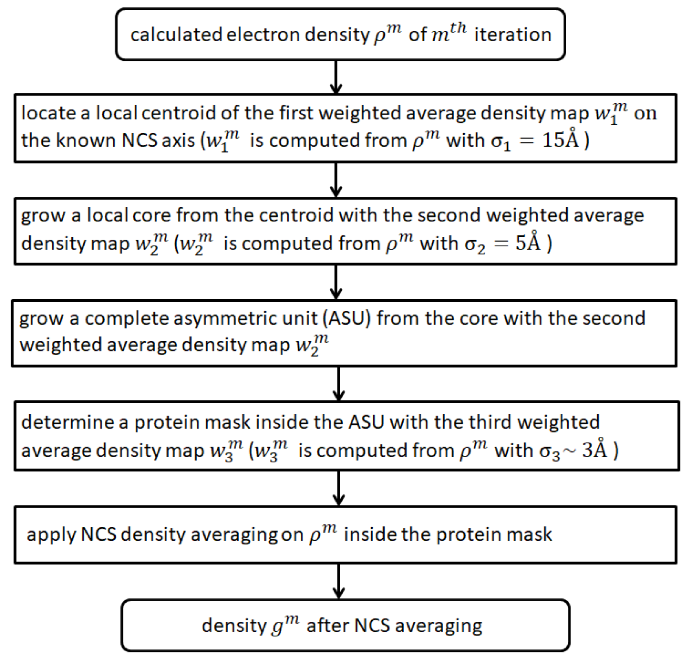
In order to apply NCS density averaging, one needs to separate the unit cell into several asymmetric units related by crystallographically symmetric operations, each ASU contains a complete protein polymer, such as a trimer or a dimer. In order to obtain the ASU, we grow it in three steps. The first step is to search for the center of the ASU, a point on the NCS axis. The second step is to grow a core surrounding the center of the ASU. The third step is to grow a complete ASU surrounding the core. When the ASU is obtained, an NCS mask is cut from the ASU to comply with the solvent content of the crystal. The mask can be used for NCS density averaging.
To describe the operations involved in the reconstruction of the NCS mask in each iteration, take a protein trimer in the space group as an example. There are four crystallographically equivalent asymmetric units in one unit cell and each asymmetric unit contains a protein trimer. Suppose the calculated density of a unit cell is ready for density modification. In order to separate the unit cell into four asymmetric units and make each ASU contain a complete protein trimmer, we grow the ASU in three steps.
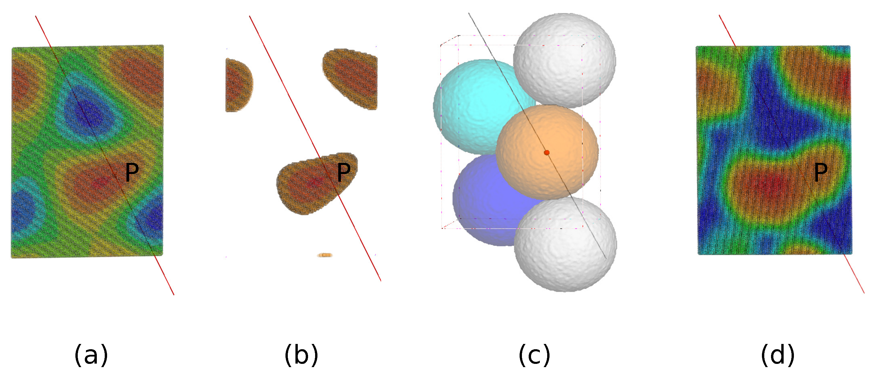
The first step is to determine a center of the trimer (the centroid) with the help of a weighted average density map as shown in Figure 1a, computed through a convolution of the calculated density with a weight given by Equation (1) with Å. It is known empirically that such a weighted average density map tends to have a maximum density near the centroid.
Since the centroid is supposed to be located on the NCS axis, we adopt the following strategy: All grid points which have a weighted average density in the top 20% range are recorded as shown in Figure 1b. For any point P on the NCS axis, a sphere is drawn with a radius so that the sphere barely touches its three crystallographic-symmetry copies as shown in Figure 1c. Now, add up all the recorded weighted average densities within this sphere. The point P with the highest total density is taken to be the centroid.
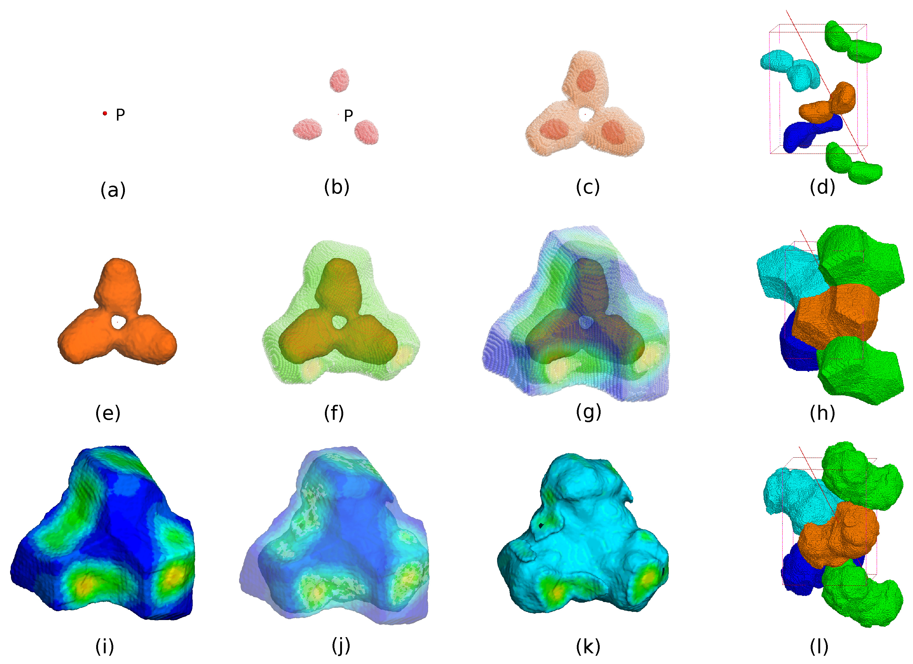
The second step is to construct a core region surrounding the center of the trimmer. Another weighted average density map with Å is employed as shown in Figure 1d. The radius of the weight distribution is much smaller than that of , therefore a more detailed structure can be revealed. In particular, the map should be able to distinguish the protein region from the solvent region. We group all the grid points of a conventional asymmetric unit into 300 bins in descending order of the weighted average density. For crystallographically equivalent grid points in the top bin, it is quite likely that only one of them is distinctly the closest to the centroid P shown as in Figure 2a. Those grid points are defined to be part of a trimeric core as shown in Figure 2b. As one moves down the bins toward grid points with low weighted average density, there comes a bin where the closest point is no longer distinct or unique within a certain cutoff distance. We define the last bin before this happens as the boundary of the core as shown in Figure 2c. Figure 2a–d indicate the construction of the core starting from the point P.
The third step starts from the last bin of the core and moves downward. For all the remaining grid points, out of the crystallographically equivalent copies, the one which is closest to the core boundary is picked as shown in Figure 2f. All such points together with the core make up a complete asymmetric unit, as shown in Figure 2g, which hopefully contains an actual protein trimer. Figure 2e–h indicate the construction of the asymmetric unit starting from the core.
The last step is to define a mask for NCS averaging. For this step, a third weighted average density map (averaged over an approximately 3 Å radius) is computed and the protein boundary is defined inside the calculated ASU using an appropriate cutoff to comply with the solvent content of the crystal as described in the previous paper (He & Su, 2015). The protein boundary inside the ASU gives the NCS mask. This mask does not necessarily satisfy the NCS operations especially during the initial hundreds of iterations. Figure 2i–l show the construction of the NCS mask from the ASU.
A flowchart for computing the NCS mask is shown in Figure 3.
After all the previous preparations, we are ready to symmetrize the density. For every grid point inside the calculated NCS mask, the new density is defined to be the average of the densities at three equivalent points even if two of those equivalent points lie outside of the NCS mask. From here on HIO, together with histogram matching [30,31] and Fourier refinement can be applied as done previously [12].
The above operations are likely to improve an approximate density so that a more accurate centroid, center core, ASU, and NCS mask emerge after each iteration. Since the reconstruction of the NCS mask is time-consuming, one does not have to reconstruct it in each iteration. Empirically, one only needs to update the NCS mask once per 100 iterations during the initial 500 iterations and update the NCS mask once per 500 iterations after the 500th iteration. It was discovered that when starting from a random density, repeated iterations can eventually produce the correct structure. A short summary of what is carried out in a single step of the iteration runs as follows: Project the density obtained from the previous iteration onto the diffraction intensity, then use various weighted averages of the resulting density to construct the new centroid, the new ASU, and the new NCS mask. The density inside the NCS mask is then symmetrized (with respect to NCS) and modified to comply with the histogram constraint, whereas HIO is applied in the solvent region. After all the density modifications, the cycle repeats itself. It should be pointed out that our algorithm is actually a combination of various projections rather than the usual iterative projection algorithm (IPA) [1,2,3,5,6,9,10,11], which is symmetric with respect to different constraints.
2.3. 3-Fold Rotational NCS
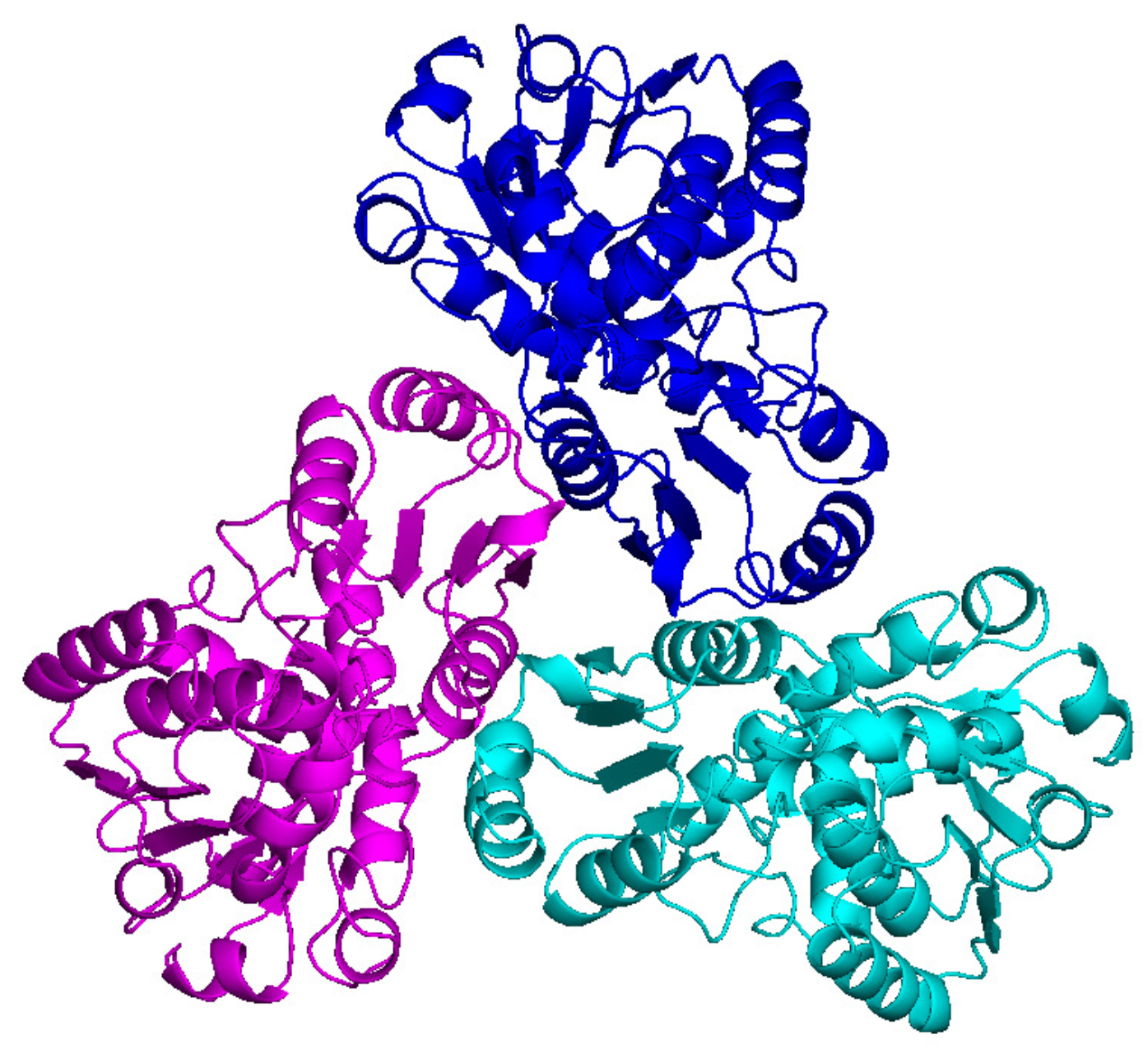
The first trial structure is a carbamoyltransferase structure with PDB code 4NF2. As shown in Figure 4, it has a 3-fold rotational NCS and there are 340 amino acids in each monomer. The cell dimensions are a = 85.89 Å, b = 99.89 Å, and c = 118.99 Å. The resolution of the diffraction data ranges from 29.23 Å to 1.74 Å with a data completeness of 99.4%. The work and free R values are 0.145 and 0.170, respectively. The solvent content is about 45%. Since there is a 3-fold NCS, the constraint ratio is about 1.72 [25,26,27] and the phase problem is well determined, and is adequate for HIO phasing method.
With the above specifications of our phasing algorithm, when applied to 4NF2, it produces the evolutions of error metrics in Figure 5. We made 200 independent runs starting from random phases and got 50 successful runs. The success rate was about 25%. The final mean phase error of a successful run was about 49 which could be further reduced to 39 by averaging over the successful runs [15] as shown in Figure 6. The final density is good enough for automatic model building by ARP/wARP [34]. Over 90% of amino acids could be correctly rebuilt. The rebuilt model matches the PDB deposited model quite well. The calculated centroid, center core, ASU, and protein boundary of a successful run of 4NF2 are shown in Figure 7.
It is instructive to track the movement of the centroid of the trimer along the NCS axis, as depicted in Figure 8. The centroid has traveled quite a distance before it settles down after 3000 iterations for one successful run, accompanied by the corresponding sharp drop in and . When the centroid of a specific run reached the correct location, the phases converged simultaneously. It is necessary but not sufficient for a run to reach the solution when the centroid has moved to the correct position. We performed another test run by fixing the centroid at the correct position. In that case, we got about 110 successful runs among 200 independent runs starting from random phases. The success rate was about 55%. The correct location of the centroid doubles the success rate.
The evolutions of the calculated center core, ASU, and protein boundary are also very interesting to observe. Figure 9 shows the calculated center core, ASU, and protein boundary of a successful run before and after it reaches the solution. Before a run reaches the solution, the calculated center core often looks featureless and sometimes even not connected. The corresponding ASU does not contain a complete trimer. As a result, the protein boundary is not correct at all. However, when a run reaches the solution, the calculated center core has already shown the 3-fold rotational symmetry. The three copies of the protein are clearly visible in the core. The resulted ASU contains one and only one complete trimer. The protein boundary becomes very accurate. In contrast, for a 2-fold NCS, as we’re going to see, individual copies cannot always be identified from the dimer core profile.
2.4. 2-Fold Rotational NCS
Twofold rotational NCS is very common in protein structures. As an example, the second trial structure is a human orotidine with PDB code 2V30. The PDB deposited structure is shown in Figure 10. The space group is . There are 279 amino acids in a single monomer and the cell dimensions are a = 60.10 Å, b = 77.85 Å, and c = 153.21 Å. The crystal diffracts from 19.64 Å to 2 Å. The solvent content is about 53%.
In the calculation, all parameters except the 2-fold NCS are the same as those ones in the previous 3-fold trial calculation. We suppose the 2-fold NCS axis is known, then we made 200 independent runs starting from random phases and got 53 successful runs. The success rate was about 26%. The calculated dimer core, ASU, and protein boundary of a successful run are shown in Figure 11. The final phase error was about 35 which is good enough for automatic model building.
3. Improper NCS
Besides proper NCS, improper NCS is also common in protein structures. The last trial structure is a lipase mutant with PDB code 5AP9 [35]. The space group is . There are 269 amino acids in each monomer and the cell dimensions are a = 90.48 Å, b = 90.48 Å, and c = 160.46 Å. The resolution range of the diffraction data is from 50 Å to 1.8 Å. The solvent fraction is about 56%.
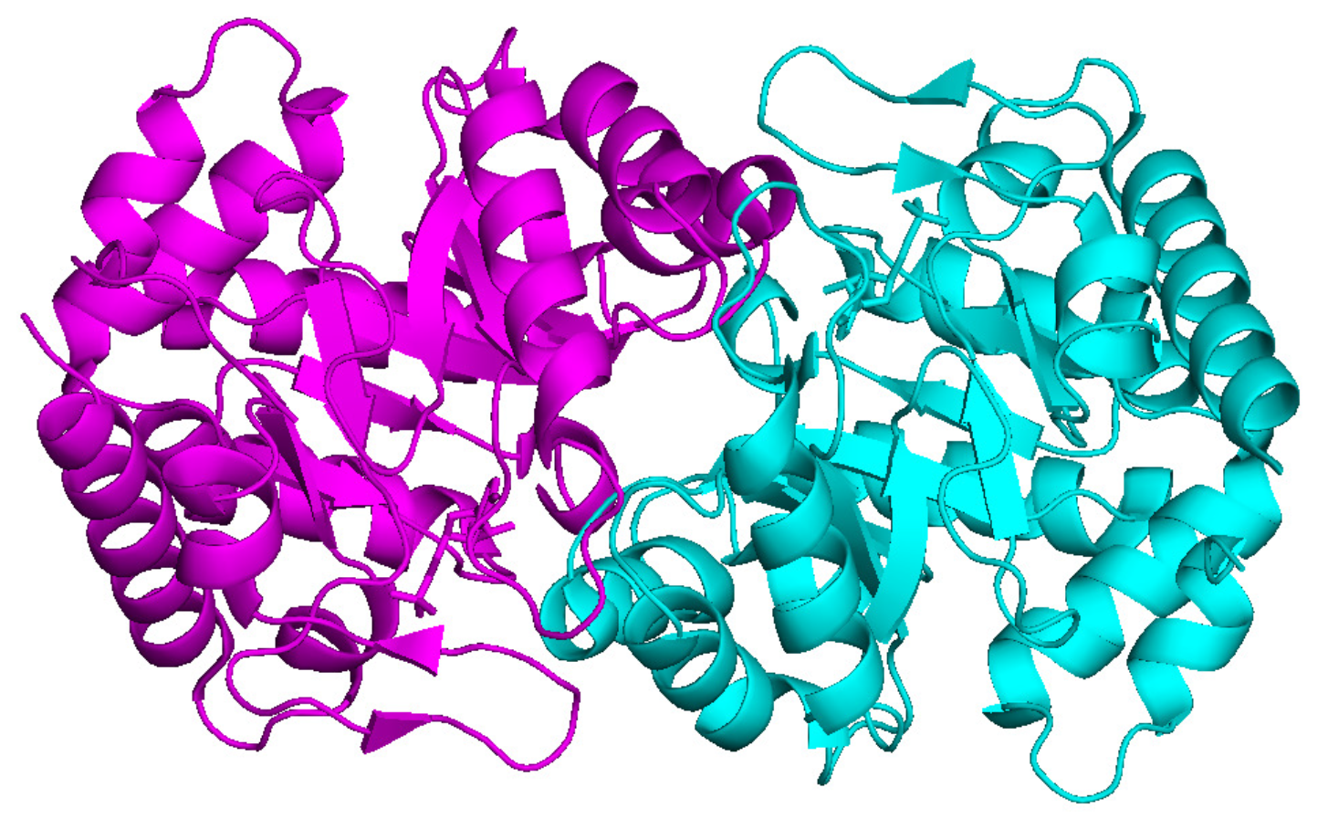
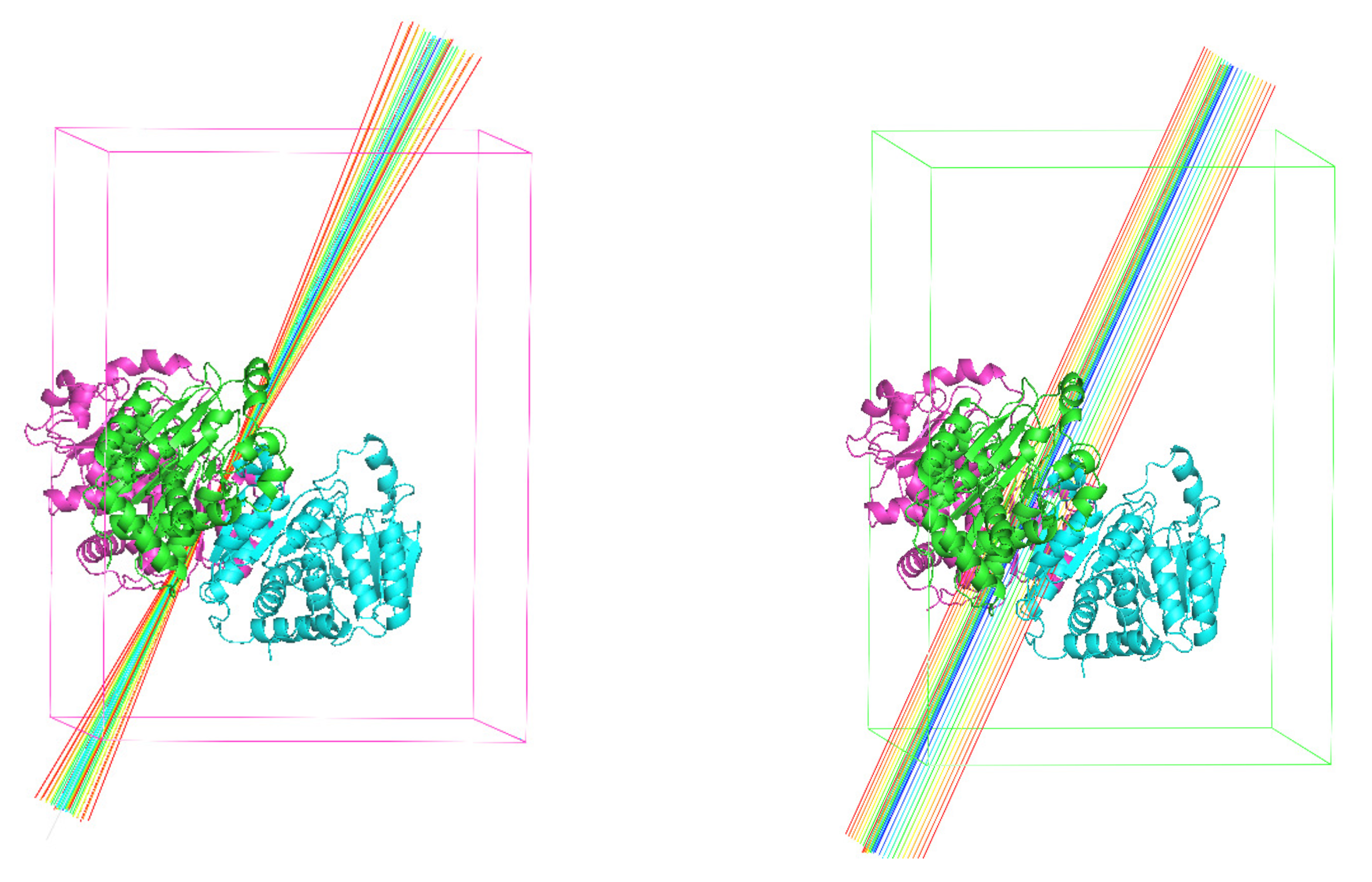
As shown in Figure 12, the purple monomer (chain A) of 5AP9, when rotated about 185.3 around the vertical axis and translated about 19.9 Å along the same axis, coincides with the cyan monomer (chain B). This operation is designated as G. Its inverse operation has to be applied to map chain B onto chain A. The choice of translation is not unique. We have chosen it to be parallel to the rotational axis.
With the symmetry operations specified, the same parameters (used for 4NF2) are followed to construct a core, extend the core into a complete ASU, and to trace the corresponding protein boundary. To carry out NCS averaging, unlike the case of a 2-fold rotational NCS (where one simply rotates every point P1 inside the NCS mask through 180 to another point P2 and average the densities at P1 and P2), for improper NCS, one needs to know which region (of chain A) to apply the operation G to as well as which region (of chain B) to apply the operation to. In other words, one needs to divide the original ASU into two equivalent halves.
To accomplish that, we use a weighted average density map with Å to search for a highest average density point P off the rotation axis. Another NCS related point Q is then generated. A core is grown gradually surrounding P, with another equivalent core surrounding Q. The growth is stopped when the two cores start to overlap. From those two cores, masks of the protein monomers can be determined (from the boundary constructed before). The two operations G and are then applied to those two masks, respectively, for the symmetrization of the protein density.
The evolution of the error metrics are displayed in Figure 13. We got 20 successful runs among 200 starting from random phases. The final phase error was about 35 after averaging over the successful runs. The centroids of most failed runs deviate from the correct positions. We also tested the case when the centroids of the monomers are given, the success rate increased a lot and we got over 100 successful runs among 200 starting from random phases.
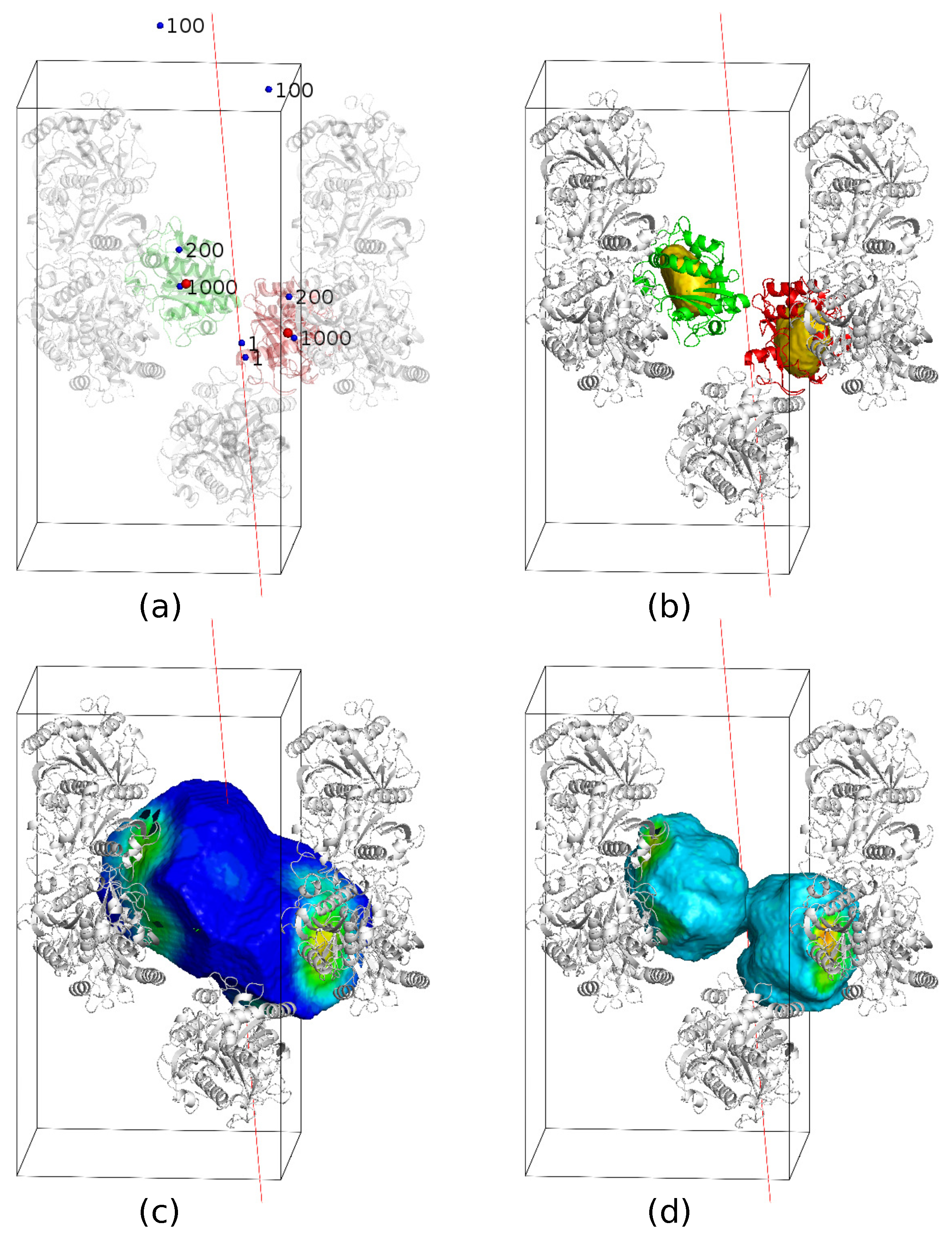
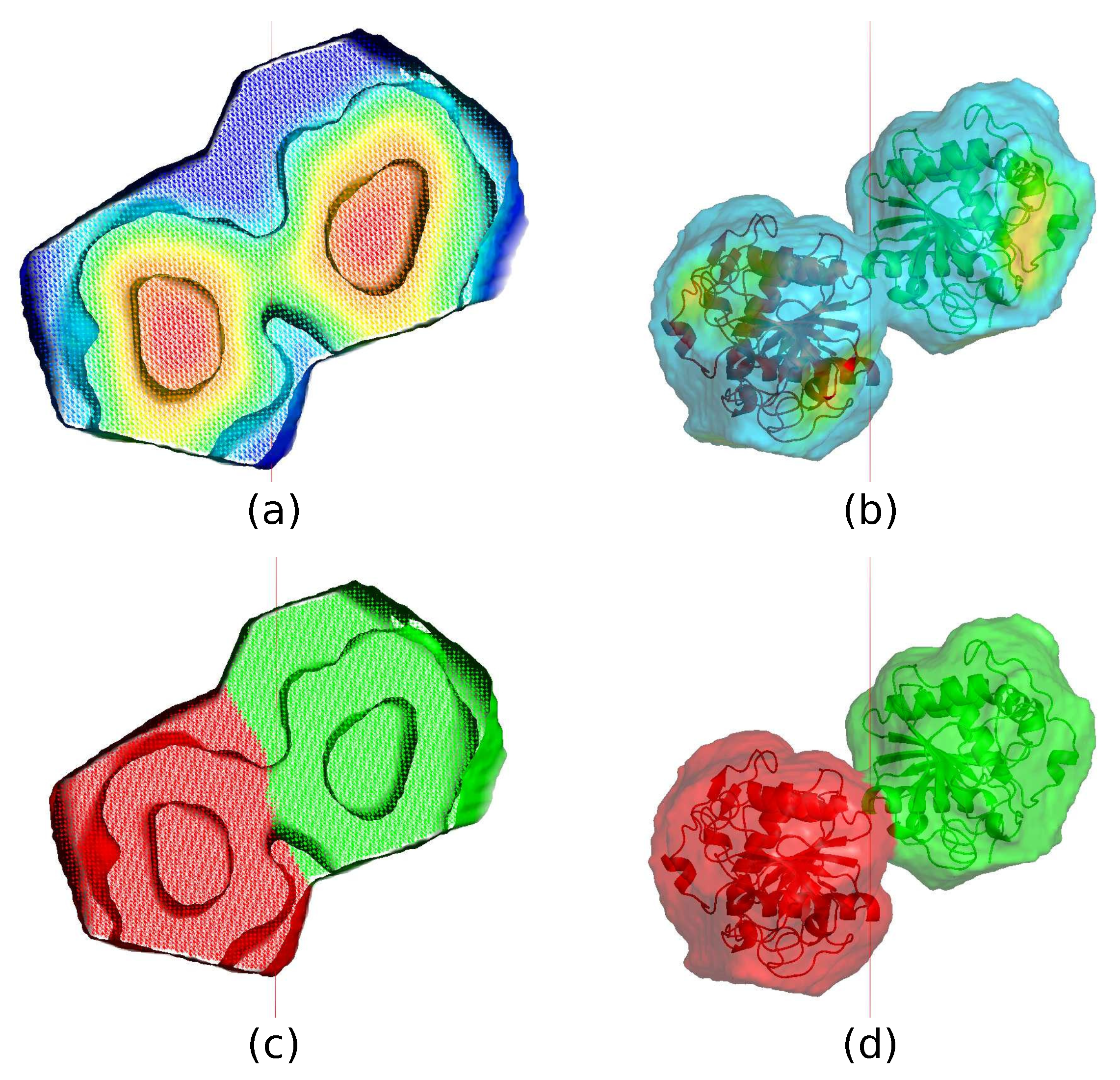
Figure 14 shows the calculated centroids, constructed core, ASU, and protein boundary. As a result of the translational operation, the core splits into two parts and each part contains a centroid.
The two calculated centroids help separate the complete ASU and protein boundary into two halves. Each half ASU contains one and only one monomer. The protein boundary clearly show the border of each monomer in Figure 15. In the final converged configuration, the two monomers show minimal contact (being almost point-like).
Table 1 is a summary of the results of all trial structures, including 4NF2, 2V30, 4Z27 [36], 1SW3 [37], and 5AP9. The solvent content of these proteins is around 50%. The final phase error was less than 40. The calculated density maps are good enough for automatic model building using ARP/wARP [34]. On average, over 90% amino acids could be correctly placed. Figure 16 shows the calculated density maps and the automatically rebuilt models of those structures with their PDB deposited structures superimposed. The reconstructed models could be further refined by CCP4 [38] and PHENIX [39].
4. Discussion
It is well-known that the direction of the NCS axis can be determined from the Patterson self rotation map. In the trial calculations, we assumed the direction of the NCS axes to be accurate. In practice, an accurate direction is often not available. One can get only an approximate direction. We need to test the tolerance of the accuracy of the axis orientation as shown in Figure 17. Take 4NF2 as an example, we allowed the axis to deviate from the correct direction by 5 initially. After each iteration, we adjust the direction of the axis to make the calculated density to better satisfy the NCS symmetry. With this optimization, we still got several successful runs, but the phase error increased a little bit. When the deviation increases to more than 5, it is difficult to reach or even get close to the correct solution.
Throughout the trial calculations, we also assumed that the location of the rotational NCS axis was given beforehand. There are some methods to identify NCS symmetry from phased density maps [24,40]. Ideally, one would like to be able to generate this through the iterations starting from a random location. We did not manage achieve that. In the mean time, one can carry out many independent parallel calculations until one of them converges as a result of the accidentally correct choice of the location of the symmetric axis, a binary map might also provide an approximate location [41], thus narrowing down the choice. We also completed some tests with the NCS axis misplaced. For example, we shifted the NCS axis of 4NF2 by 10 Å as shown in Figure 17. By updating the location of the axis, each iteration optimized the NCS symmetry, and we got some successful runs. However, when the deviation becomes larger, the solution can not be reached.
If neither the orientation nor the location is accurate, a search should be applied in six dimensions. For 4NF2, we carried out a trial calculation with an initial orientational error of 5 and locational error of 5 Å, the orientation and the location being updated through the iterations. Out of 400 runs, we found that the location and orientation both converged to the correct results in one run. More extensive tests remain to be carried out to evolve the orientation and location of the NCS axes. The corresponding problem for improper NCS also needs to be addressed.
5. Conclusions
Although phasing of most protein crystals can be routinely done through standard methodologies such as molecular replacement and anomalous scattering, the availability of a direct phasing algorithm would certainly be very beneficial, even becoming critical when standard methods fail.
A direct phasing algorithm based on HIO has proved to work for high solvent content protein crystals, typically for a solvent content higher than 65%. Statistically the chance of running into such a protein crystal is about 10%. Therefore, the applicability of the HIO method is severely limited. In this paper, we have shown through trial calculations that with the presence of NCS, structures with an average solvent concentration are amenable to the HIO approach. Therefore, because a significant fraction (about 40%) of protein crystals possess NCS, HIO direct phasing is a practically useful tool.
Precise information regarding the NCS operation was assumed in our trial calculations, however, the prospect of deriving this information from the diffraction data is good.
Author Contributions
H.H. and W.-P.S. conceived the concepts; H.H. and M.J. carried out the calculations; H.H. and W.-P.S. wrote the paper.
Funding
This research was funded by the Robert A. Welch Foundation (under grant number E-1070) and the Texas Center for Superconductivity at the University of Houston.
Acknowledgments
This work was partially supported by the Texas Center for Superconductivity and the Robert A. Welch Foundation (E-1070). The authors acknowledge the use of the Maxwell/Opuntia Cluster and the advanced support from the Center for Advanced Computing and Data Systems at the University of Houston, and the use of the Galcano Cluster of Chin-Sen Ting’s group at the University of Houston to carry out the research presented here.
Conflicts of Interest
The authors declare no conflict of interest. The founding sponsors had no role in the design of the study; in the collection, analyses, or interpretation of data; in the writing of the manuscript, and in the decision to publish the results.
References
- Fienup, J.R. Reconstruction of an object from the modulus of its Fourier transform. Opt. Lett. 1978, 3, 27–29. [Google Scholar] [CrossRef]
- Millane, R.P. Phase retrieval in crystallography and optics. J. Opt. Soc. Am. 1990, 7, 394–411. [Google Scholar] [CrossRef]
- Elser, V. Phase retrieval by iterated projections. J. Opt. Soc. Am. A 2003, 20, 40–55. [Google Scholar] [CrossRef]
- Elser, V. Solution of the crystallographic phase problem by iterated projections. Acta Cryst. A 2003, 59, 201–209. [Google Scholar] [CrossRef] [Green Version]
- Marchesini, S.; He, H.; Chapman, H.N.; Hau-Riege, S.P.; Noy, A.; Howells, M.R.; Weierstall, U.; Spence, J.C.H. X-ray image reconstruction from a diffraction pattern alone. Phys. Rev. B 2003, 68, 140101. [Google Scholar] [CrossRef] [Green Version]
- Marchesini, S. Invited Article: A unified evaluation of iterative projection algorithms for phase retrieval. Rev. Sci. Instrum. 2007, 78, 011301. [Google Scholar] [CrossRef] [PubMed]
- Lo, V.L.; Millane, R.P. Reconstruction of compact binary images from limited Fourier amplitude data. J. Opt. Soc. Am. A 2008, 25, 2600–2607. [Google Scholar] [CrossRef]
- Liu, Z.C.; Xu, R.; Dong, Y.H. Phase retrieval in protein crystallography. Acta Cryst. A 2012, 68, 256–265. [Google Scholar] [CrossRef] [PubMed]
- Millane, R.P.; Lo, V.L. Iterative projection algorithms in protein crystallography. I. Theory. Acta Cryst. A 2013, 69, 517–527. [Google Scholar] [CrossRef]
- Lo, V.L.; Kingston, R.L.; Millane, R.P. Iterative projection algorithms in protein crystallography. II. Application. Acta Cryst. A 2015, 71, 451–459. [Google Scholar] [CrossRef]
- Lo, V.L.; Kingston, R.L.; Millane, R.P. Iterative projection algorithms for ab initio phasing in virus crystallography. J. Struct. Biol. 2016, 196, 407–413. [Google Scholar] [CrossRef] [PubMed]
- He, H.; Su, W.-P. Direct phasing of protein crystals with high solvent content. Acta Cryst. A 2015, 71, 92–98. [Google Scholar] [CrossRef]
- He, H.; Fang, H.; Miller, M.D.; Phillips, G.N., Jr.; Su, W.-P. Improving the efficiency of molecular replacement by utilizing a new iterative transform phasing algorithm. Acta Cryst. A 2016, 72, 539–547. [Google Scholar] [CrossRef] [PubMed] [Green Version]
- He, H.; Su, W.-P. Improving the convergence rate of a hybrid input-output phasing algorithm by varying the reflection data weight. Acta Cryst. A 2018, 74, 36–43. [Google Scholar] [CrossRef] [PubMed]
- Jiang, M.C.; He, H.X.; Cheng, Y.P.; Su, W.-P. Resolution Dependence of an Ab Initio Phasing Method in Protein X-ray Crystallography. Crystals 2018, 8, 156. [Google Scholar] [CrossRef]
- Fienup, J.R. Phase retrieval algorithms: A comparison. Appl. Opt. 1982, 21, 2758–2769. [Google Scholar] [CrossRef]
- Liu, Z.C. Iterative Method of Phase Retrieval in Protein Crystallography. Ph.D. Thesis, Institute of High Energy Physics, Chinese Academy of Sciences, Beijing, China, 2012. [Google Scholar]
- Bricogne, G. Geometric sources of redundancy in intensity data and their use for phase determination. Acta Cryst. A 1974, 30, 395–405. [Google Scholar] [CrossRef] [Green Version]
- Rossmann, M.G. Ab initio phase determination and phase extension using non-crystallographic symmetry. Curr. Opin. Struct. Biol. 1995, 5, 650–655. [Google Scholar] [CrossRef]
- Schuller, D.J. MAGICSQUASH: More Versatile Non-crystallographic Averaging with Mulitple Constraints. Acta Cryst. D 1996, 52, 425–434. [Google Scholar] [CrossRef]
- Cowtan, K.D.; Zhang, K.Y.J.; Main, P. International Tables for Crystallography; Arnold, E., Rossmann, M.G., Eds.; Kluwer Academic Publishers: Dordrecht, The Netherlands, 2001; Volume F, Chapter 25.2.5. [Google Scholar]
- Terwilliger, T.C. Statistical density modification with non-crystallographic symmetry. Acta Cryst. D 2002, 58, 2082–2086. [Google Scholar] [CrossRef] [Green Version]
- Terwilliger, T.C. Rapid automatic NCS identification using heavy-atom substructures. Acta Cryst. D 2002, 58, 2213–2215. [Google Scholar] [CrossRef] [Green Version]
- Terwilliger, T.C. Finding non-crystallographic symmetry in density maps of macromolecular structures. J. Struct. Funct. Genom. 2013, 14, 91–95. [Google Scholar] [CrossRef] [PubMed] [Green Version]
- Miao, J.; Sayer, D.; Chapman, H.N. Phase retrieval from the magnitude of the Fourier transforms of non-periodic objects. J. Opt. Soc. Am. 1998, 15, 1662–1669. [Google Scholar] [CrossRef]
- Elser, V.; Millane, R.P. Reconstruction of an object from its symmetry-averaged diffraction pattern. Acta Cryst. A 2008, 64, 273–279. [Google Scholar] [CrossRef] [PubMed] [Green Version]
- Millane, R.P.; Arnal, R.D. Uniqueness of the macromolecular crystallographic phase problem. Acta Cryst. A 2015, 71, 592–598. [Google Scholar] [CrossRef] [PubMed]
- Vellieux, F.M.D.A.P.; Hunt, J.F.; Roy, S.; Read, R.J. DEMON/ANGEL: A suite of programs to carry out density modification. J. Appl. Cryst. 1995, 28, 347–351. [Google Scholar] [CrossRef]
- Cowtan, K.; Main, P. Miscellaneous algorithms for density modifiation. Acta Cryst. D 1998, 54, 487–493. [Google Scholar] [CrossRef]
- Zhang, K.Y.J.; Main, P. Histogram matching as a new density modification technique for phase refinement and extension of protein molecules. Acta Cryst. A 1990, 46, 41–46. [Google Scholar] [CrossRef] [Green Version]
- Zhang, K.Y.J.; Main, P. The use of Sayre’s equation with solvent flattening and histogram matching for phase extension and refinement of protein structures. Acta Cryst. A 1990, 46, 377–381. [Google Scholar] [CrossRef]
- Wang, B.C. Resolution of phase ambiguity in macromolecular crystallography. Methods Enzymol. 1985, 115, 90–112. [Google Scholar] [CrossRef]
- Brünger, A.T. Free R value: A novel statistical quantity for assessing the accuracy of crystal structures. Nature 1992, 355, 472–475. [Google Scholar] [CrossRef]
- Langer, G.G.; Cohen, S.X.; Lamzin, V.S.; Perrakis, A. Automated macromolecular model building for X-ray crystallography using ARP/wARP version 7. Nat Protoc. 2008, 3, 1171–1179. [Google Scholar] [CrossRef] [PubMed] [Green Version]
- Skjold-Jrgensen, J.; Vind, J.; Moroz, O.V.; Blagova, E.; Bhatia, V.K.; Svendsen, A.; Wilson, K.S.; Bjerrum, M.J. Controlled lid-opening in Thermomyces lanuginosus lipase—An engineered switch for studying lipase function. Biochim. Biophys. Acta 2017, 1865, 20–27. [Google Scholar] [CrossRef] [PubMed]
- Avraham, O.; Meir, A.; Fish, A.; Bayer, E.A.; Livnah, O. Hoefavidin: A dimeric bacterial avidin with a C-terminal binding tail. J. Struct. Biol. 2015, 191, 139–148. [Google Scholar] [CrossRef] [PubMed]
- Kursula, I.; Salin, M.; Sun, J.; Norledge, B.V.; Haapalainen, A.M.; Sampson, N.S.; Wierenga, R.K. Understanding protein lids: Structural analysis of active hinge mutants in triosephosphate isomerase. Protein Eng. Des. Sel. 2004, 17, 375–382. [Google Scholar] [CrossRef]
- Winn, M.D.; Ballard, C.C.; Cowtan, K.D.; Dodson, E.J.; Emsley, P.; Evans, P.R.; Keegan, R.M.; Krissinel, E.B.; Leslie, A.G.W.; McCoy, A.; et al. Overview of the CCP4 suite and current developments. Acta. Cryst. D 2011, 67, 235–242. [Google Scholar] [CrossRef] [PubMed]
- Adams, P.D.; Afonine, P.V.; Bunkóczi, G.; Chen, V.B.; Davis, I.W.; Echols, N.; Headd, J.J.; Hung, L.-W.; Kapral, G.J.; Grosse-Kunstleve, R.W.; et al. PHENIX: A comprehensive Python-based system for macromolecular structure solution. Acta Cryst. D 2010, 66, 213–221. [Google Scholar] [CrossRef]
- Pai, R.; Sacchettini, J.; Ioerger, T. Identifying non-crystallographic symmetry in protein electron-density maps: A feature-based approach. Acta Cryst D 2006, 62, 1012–1021. [Google Scholar] [CrossRef]
- Su, W.-P. Retrieving low- and medium-resolution structural features of macromolecules directly from the diffraction intensities—A real-space approach to the X-ray phase problem. Acta Cryst. A 2008, 64, 625–630. [Google Scholar] [CrossRef]
Figure 1.
(a) A section of the weighted average density map with Å. The red color represents high-density regions and the blue color indicates low-density regions. (b) From , weighted average densities in the top 20% are recorded. (c) For any point P on the non-crystallographic symmetry (NCS) axis, a sphere is drawn with a radius so that the sphere barely touches its crystallographic-symmetry copies indicated by different colors. (d) After updating the centroid, another weighted average density map is computed with Å. A mask for NCS averaging can be constructed from .

Figure 2.
An example of the construction of the core, asymmetric unit (ASU), and NCS mask. (a) The updated centroid P. (b) High-density region of the core. (c) A complete core. (d) The core and its crystallographic-symmetry copies indicated by different colors. (e) The boundary of the core. (f) Grid points close to the core boundary. (g) All grid points close to the core boundary together with the core make up a new complete asymmetric unit. (h) The new asymmetric unit and its crystallographic-symmetry copies. (i) The boundary of the new asymmetric unit. Warm color represents high-density regions and cool color indicates low-density regions. (j) An NCS mask is defined inside the new asymmetric unit by an appropriate cutoff value based on a third weighted average density map with around . (k) The new NCS mask. (l) The NCS mask and its crystallographic-symmetry copies.

Figure 3.
A flowchart for computing the NCS mask.

Figure 4.
PDB deposited model of 4NF2. The 3-fold NCS axis is perpendicular to the plane of the paper.
Figure 4.
PDB deposited model of 4NF2. The 3-fold NCS axis is perpendicular to the plane of the paper.

Figure 5.
Direct phasing of 4NF2 with NCS averaging. The evolution of error metrics starting from random phases: (a) free R-value, (b) mean phase error, and (c) correlation coefficient.
Figure 5.
Direct phasing of 4NF2 with NCS averaging. The evolution of error metrics starting from random phases: (a) free R-value, (b) mean phase error, and (c) correlation coefficient.

Figure 6.
The phase error and CC value after averaging over those successful runs of 4NF2.

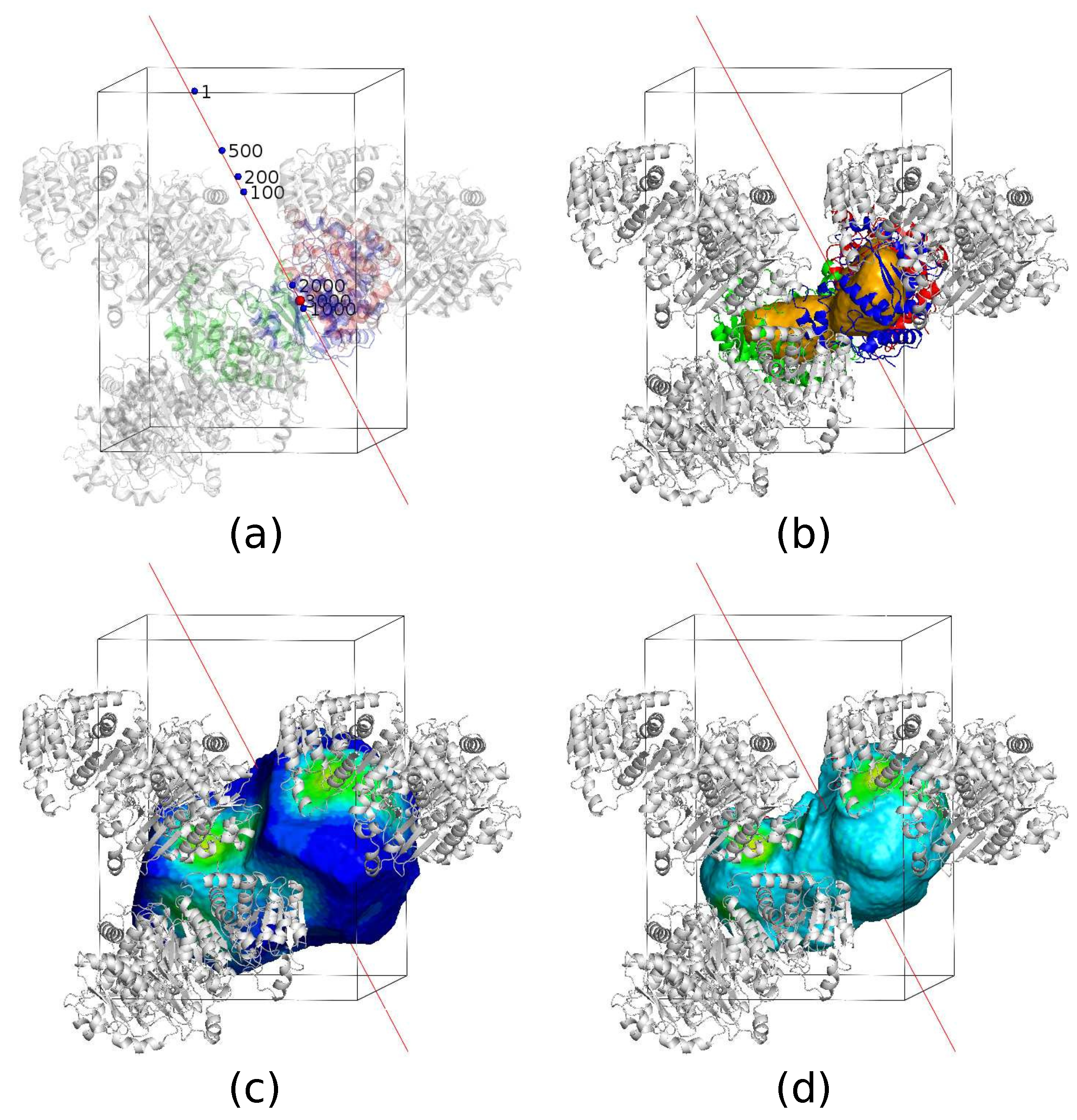
Figure 7.
The calculated (a) centroid, (b) center core, (c) ASU, and (d) protein boundary of a typical successful run of 4NF2. The known 3-fold NCS axis (red line) pierces through the unit cell. The PDB deposited model of 4NF2 and its symmetric copies are shown as gray. (a) Blue spheres on the NCS axis show the evolution of the calculated centroid with the number of the iteration. At the 3000th iteration, the calculated centroid has evolved to the correct position (shown as a red sphere), and no longer moves away after that. At the 3000th iteration, the centroid, center core, ASU, and protein boundary become mature and are quite close to the exact ones. (b) The calculated center core of the 3000th iteration which grows from the calculated centroid in (a). (c) The calculated ASU of the 3000th iteration. The ASU grows from the center core and it contains one and only one complete trimer. (d) The calculated protein boundary of the 3000th iteration. The protein boundary is located inside the ASU.

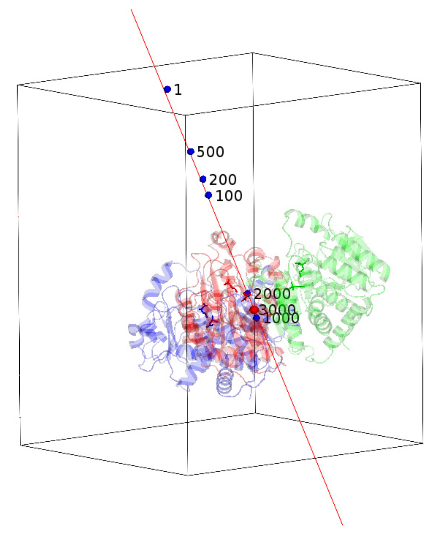
Figure 8.
The blue spheres near the known NCS axis represent the locations of the calculated centroid of a successful run of 4NF2. The label shows the number of iterations. The initial position of the calculated centroid is random and far away from the correct position shown as the red sphere. At the 1000th iteration, it gets quite close to the correct position. At the 3000th iteration, it reaches the correct position and stays there after that.

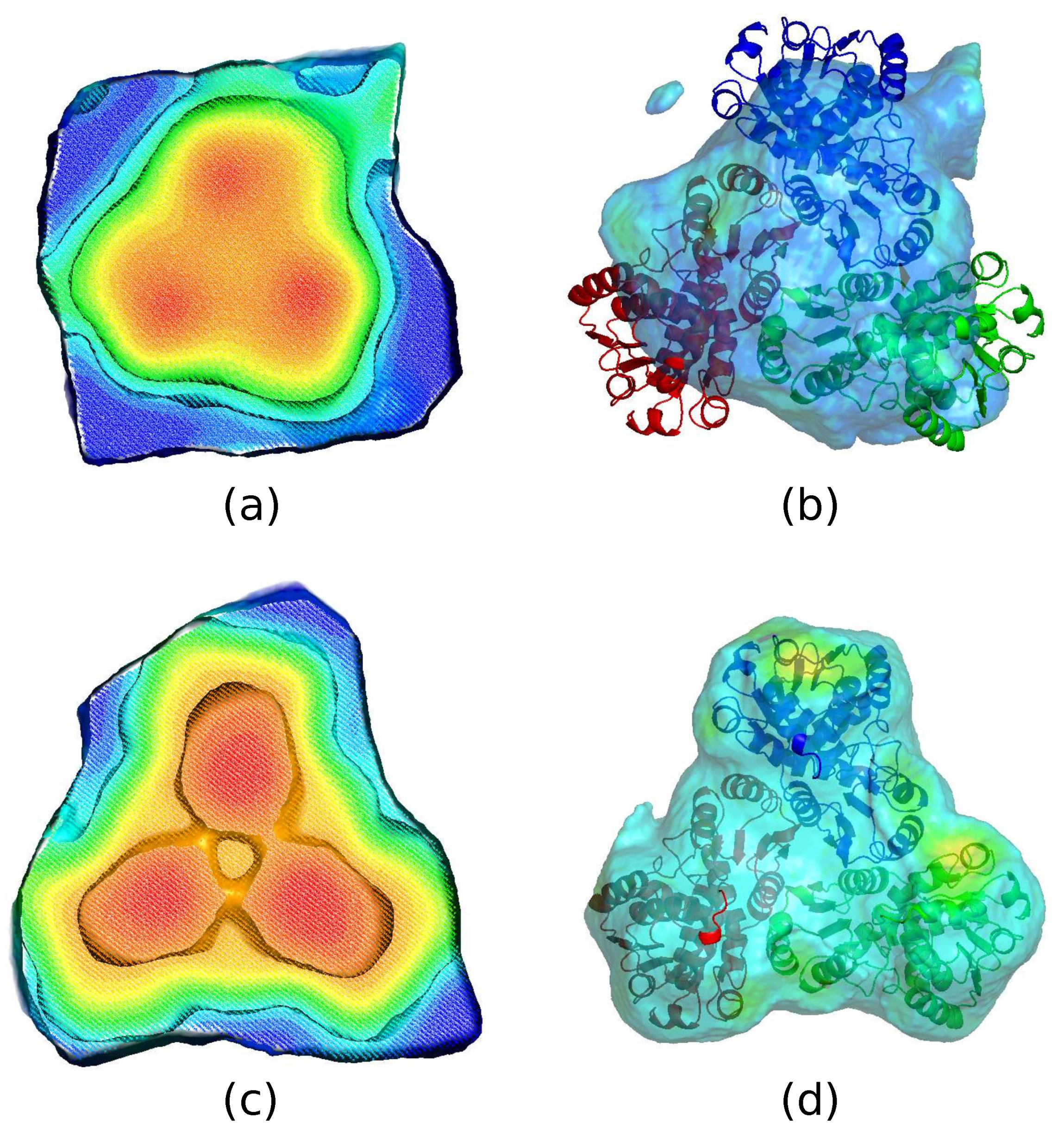
Figure 9.
Evolution of the calculated core, ASU, and protein boundary of 4NF2 in a successful run. Warm colors represents high weighted average density. (a,b) Show the calculated center core, ASU, and protein boundary before a run reaches the solution. The inner shell shows the center core region. The outer shell corresponds to a complete asymmetric unit building from the core towards the gradient direction on a weighted average density map. The protein boundary shown as the middle shell is contained inside the calculated ASU. (c,d) Show the results after the run reaches the solution. The calculated protein boundary matches the PDB deposited model very well.

Figure 10.
PDB deposited model of 2V30. The 2-fold NCS axis is perpendicular to the plane of the paper.
Figure 10.
PDB deposited model of 2V30. The 2-fold NCS axis is perpendicular to the plane of the paper.

Figure 11.
The calculated dimer core, ASU, and protein boundary of 2V30 in a successful run. The 2-fold NCS axis is perpendicular to the plane of the paper.
Figure 11.
The calculated dimer core, ASU, and protein boundary of 2V30 in a successful run. The 2-fold NCS axis is perpendicular to the plane of the paper.

Figure 12.
PDB deposited model of 5AP9. The rotational NCS axis is parallel to the translation.

Figure 13.
Evolution of the error metrics of 5AP9 starting from random phases. (a) Free R-value, (b) mean phase error, and (c) correlation coefficient.
Figure 13.
Evolution of the error metrics of 5AP9 starting from random phases. (a) Free R-value, (b) mean phase error, and (c) correlation coefficient.

Figure 14.
The calculated centroids, core, ASU, and protein boundary of 5AP9 from a typical successful run.
Figure 14.
The calculated centroids, core, ASU, and protein boundary of 5AP9 from a typical successful run.

Figure 15.
(a,b) Show the constructed dimer core, ASU, and protein boundary of 5AP9. Warm colors in (a,b) represent high weighted average density. (c,d) Show the monomers.
Figure 15.
(a,b) Show the constructed dimer core, ASU, and protein boundary of 5AP9. Warm colors in (a,b) represent high weighted average density. (c,d) Show the monomers.

Figure 16.
The calculated density map (gray mesh) and the reconstructed model (green sticks) with the PDB deposited model (red sticks) superimposed. The model was rebuilt with ARP/wARP [34].
Figure 16.
The calculated density map (gray mesh) and the reconstructed model (green sticks) with the PDB deposited model (red sticks) superimposed. The model was rebuilt with ARP/wARP [34].

Figure 17.
Variation of the 3-fold NCS axis of 4NF2 in orientation and location for testing the tolerance of the HIO algorithm.
Figure 17.
Variation of the 3-fold NCS axis of 4NF2 in orientation and location for testing the tolerance of the HIO algorithm.


Table 1.
Results of the trial calculations.
| PDB Code | Space Group | # of Amino Acids | NCS Copies in ASU | Solvent Content (%) | Data Resolution (Å) | Phase Error () | Model Completeness (%) |
|---|---|---|---|---|---|---|---|
| 4NF2 | 340 | 3 | 45 | 1.74 | 39 | 87 | |
| 2V30 | 279 | 2 | 53 | 2.00 | 35 | 91 | |
| 4Z27 | 134 | 2 | 55 | 1.34 | 30 | 88 | |
| 1SW3 | 248 | 2 | 55 | 2.03 | 35 | 98 | |
| 5AP9 | 269 | 2 | 56 | 1.80 | 35 | 90 |
© 2019 by the authors. Licensee MDPI, Basel, Switzerland. This article is an open access article distributed under the terms and conditions of the Creative Commons Attribution (CC BY) license (http://creativecommons.org/licenses/by/4.0/).
Share and Cite
MDPI and ACS Style
He, H.; Jiang, M.; Su, W.-P. Direct Phasing of Protein Crystals with Non-Crystallographic Symmetry. Crystals 2019, 9, 55. https://0-doi-org.brum.beds.ac.uk/10.3390/cryst9010055
AMA Style
He H, Jiang M, Su W-P. Direct Phasing of Protein Crystals with Non-Crystallographic Symmetry. Crystals. 2019; 9(1):55. https://0-doi-org.brum.beds.ac.uk/10.3390/cryst9010055
Chicago/Turabian StyleHe, Hongxing, Mengchao Jiang, and Wu-Pei Su. 2019. "Direct Phasing of Protein Crystals with Non-Crystallographic Symmetry" Crystals 9, no. 1: 55. https://0-doi-org.brum.beds.ac.uk/10.3390/cryst9010055
Note that from the first issue of 2016, this journal uses article numbers instead of page numbers. See further details here.