Wetting of Nematic Liquid Crystals on Crenellated Substrates: A Frank–Oseen Approach


1
Departamento de Física Atómica, Molecular y Nuclear, Área de Física Teórica, Facultad de Física, Universidad de Sevilla, Avenida de Reina Mercedes s/n, 41012 Sevilla, Spain
2
Centro de Física Teórica e Computacional, Faculdade de Ciências, Universidade de Lisboa, 1749-016 Lisboa, Portugal
3
Departamento de Física, Faculdade de Ciências, Universidade de Lisboa, 1749-016 Lisboa, Portugal
*
Author to whom correspondence should be addressed.
Crystals 2019, 9(8), 430; https://0-doi-org.brum.beds.ac.uk/10.3390/cryst9080430
Submission received: 24 July 2019
/
Revised: 5 August 2019
/
Accepted: 10 August 2019
/
Published: 19 August 2019
(This article belongs to the Special Issue Advances in Nematic Liquid Crystals)
Abstract
:We revisit the wetting of nematic liquid crystals in contact with crenellated substrates, studied previously using the Landau–de Gennes formalism. However, due to computational limitations, the characteristic length scales of the substrate relief considered in that study limited to less than 100 nematic correlation lengths. The current work uses an extended Frank–Oseen formalism, which includes not only the free-energy contribution due to the elastic deformations but also the surface tension contributions and, if disclinations or other orientational field singularities are present, their core contributions. Within this framework, which was successfully applied to the anchoring transitions of a nematic liquid crystal in contact with structured substrates, we extended the study to much larger length scales including the macroscopic scale. In particular, we analyzed the interfacial states and the transitions between them at the nematic–isotropic coexistence.
1. Introduction
The study of nematic liquid crystals in contact with microstructured substrates has been an active area of research in the last decades [1,2,3], with practical applications such as zenithally bistable devices [4,5,6,7,8,9] and tailoring of soft rails for colloidal transport on surfaces [10,11,12,13,14,15,16]. Structured substrates frustrate the nematic orientational order, and thus elastic distortions of the nematic and, in some cases, topological defects arise driven by the substrate relief. When the substrate has cusps, disclination-like singularities nucleate at or very close to them [17,18,19,20,21,22]. These play an essential role in the multistability resulting from the existence of distinct interfacial states of the nematic in contact with a microstructured substrate, with different nematic textures [23].
Nematic wetting of structured substrates has attracted much less attention [24,25]. At planar substrates, a first-order orientational wetting transition is predicted by the Landau–de Gennes theory, where a macroscopic nematic layer intrudes at the substrate–isotropic liquid interface [26,27], and has been observed experimentally [28,29,30,31,32]. Macroscopically, wetting of a planar substrate is described by Young’s equation
where is the contact angle between the planar substrate and a large nematic droplet at coexistence with the isotropic phase. Equation (1) can be understood as the force balance applied to the nematic–isotropic–substrate contact line. When the substrate is rough, the effective surface area increases. Simple thermodynamic arguments show that, under these conditions, the wetting transition should occur for a contact angle which obeys Wenzel’s law [33]
where the roughness parameter r is defined as , with the true substrate area and its projected area. This result is based on the assumption that the wetting transition involves the same interfacial states as the planar case, denoted by dry and complete wet states. However, even for simple fluids, roughness leads to the stabilization of intermediate states where the substrate grooves are partially filled while the substrate is still in contact with the bulk phase, which are denoted by filled states. In this framework, wetting phenomena become more complex, and new transitions such as filling may precede the wetting transition [34,35]. This is also expected to occur for liquid crystals. In addition, the interplay between interfacial configurations (as well as the substrate relief) and the orientational order in the nematic phase generates a plethora of distinct interfacial states, leading to rather complex interfacial phase diagrams [36]. In this context, systematic studies of the wetting for sawtooth [36,37], sinusoidal [38,39] and crenellated substrates [40,41] have been reported within the Landau–de Gennes theory. These studies revealed complex phase diagrams which differ considerably from their simple fluids counterparts. This can be ascribed to the role played by elastic deformations and the presence of topological defects in the free energy of the interfacial states. These studies were, however, restricted to substrate periodicities smaller than , where is the bulk nematic correlation length, owing to computational limitations. Thus, it is desirable to extend the analysis of the wetting phase diagrams to larger values of the substrate period to understand in detail the differences between the phenomenology for simple fluids and in nematic liquid crystals. In this paper, we extend the modified Frank–Oseen model [22] to study wetting phenomena on microstructured substrates. As an example, we apply this model to the study of the wetting phase diagram of crenellated substrates, although the methodology can be readily applied to other substrates.The modified Frank–Oseen model has been successfully applied to characterize the behavior of bulk nematic liquid crystals in contact with microstructured substrates, with results in line with those of the Landau–de Gennes theory [22,23]. This approach will bridge the gap between the macroscopic scale and the mesoscopic scale described by the Landau–de Gennes theory, shedding light on the physical mechanisms that drive wetting by nematic liquid crystals.
2. Theoretical Model and Methods
Wetting of a nematic, at equilibrium with the isotropic liquid, on a crenellated substrate with homeotropic anchoring is considered within the modified Frank–Oseen model [21,22,23]. In this model, the free energy of an interfacial configuration of the nematogen in contact with the substrate is given by three contributions. First, the surface contribution associated to the different interfaces. There are three distinct interfaces: substrate–nematic, substrate–isotropic and nematic–isotropic. We assume that the substrate anchoring is homeotropic for both nematic and isotropic phases, i.e., nematogen molecules orient preferentially perpendicular to the substrate when close to it. On the other hand, random planar anchoring at the nematic–isotropic interface is considered, that is, molecules are oriented parallel to the interface but there is no privileged orientation in the interfacial plane. We denote by , and the surface tension associated to the substrate–nematic, substrate–isotropic and nematic–isotropic interface, respectively, with the anchoring conditions mentioned above. Thus, the surface contribution can be written as
where and stand for the phases (isotropic, nematic and substrate) and is the total interfacial area between phases and . The second contribution is associated to the elastic distortions of the director field in the nematic phase. For this purpose, we suppose that anchoring is strong, i.e., the director field is fixed at the substrate and at the interface. This condition is valid if the relevant length scales at the surface and at the interface are much larger than the extrapolation length [42]. Under these conditions, the elastic contribution is given by the Frank–Oseen model [43,44]
where is the volume occupied by the nematic; , and are the splay, twist and bend bulk elastic constants, respectively; and is the saddle-splay elastic constant. Finally, if disclinations and/or director field singularities associated to cusps in the substrate topography appear in the nematic texture, a third contribution associated to the nematic order distortions in the defect or singularity cores must be included. Thus, the total free energy can be written as
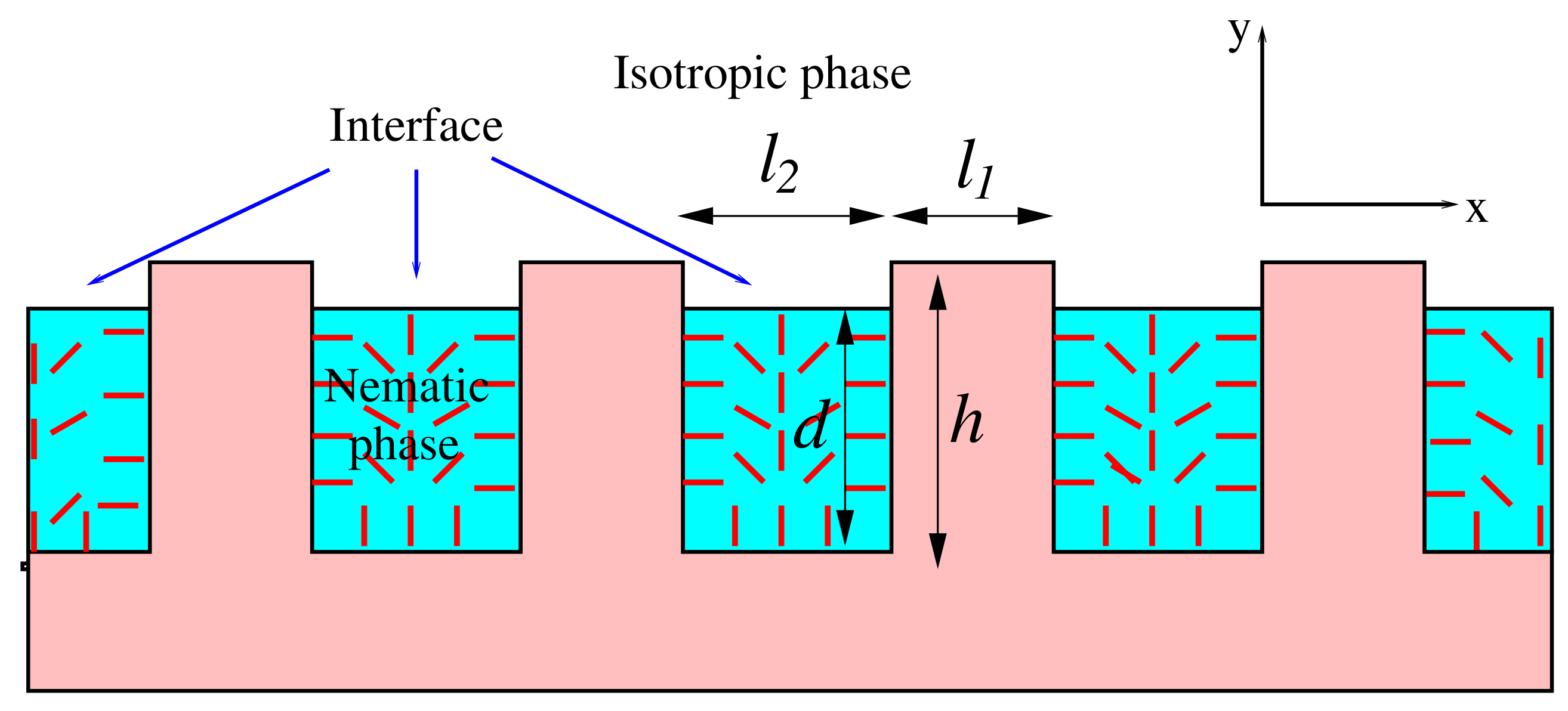
We consider a crenellated substrate with grooves of depth and width h and , respectively, separated horizontally by a distance (see Figure 1), so that the period of the substrate relief is . The substrate is translationally invariant along the z axis. The substrate promotes the nematic phase (with homeotropic anchoring, as previously stated) and is in contact with a bulk isotropic phase. Under appropriate conditions, a wetting nematic layer is formed between the substrate and the isotropic bulk phase. In general, the profile of the nematic–isotropic interface is unknown and should be obtained by the minimization of Equation (5). However, in what follows, we assume that it is planar and parallel to the plane. This approximation is valid for wide grooves, since the Laplace equation dictates that at nematic–isotropic coexistence the interfacial curvature must vanish. Within this approximation, the interfacial configuration is determined by the nematic layer thickness d, as shown in Figure 1. Furthermore, we suppose that the director field in the nematic phase is in the plane and, consequently, only splay and bend deformations are allowed. Under these simplifying assumptions, the director field can be parameterized as , and Equation (4) can be recast as [17,23]
Our goal is to obtain the wetting phase diagram of the Landau–de Gennes theory in the limit of wide grooves or large-scale surface relief. In this sense, the model outlined above can be understood as an approximation to the Landau–de Gennes theory in this limit [21,22,23]. In particular, and in order to make contact with previous results [40], we consider the following Landau–de Gennes free energy , where the bulk and elastic free energy densities are, respectively,
Here, is the traceless symmetric nematic order tensor with matrix elements [42]; denotes the trace operation; T is the temperature; , b, , and are phenomenological constants; is the partial derivative with respect to the Cartesian coordinate ; and Einstein summation convention in Equation (8) is used. The bulk term , which accounts for the contribution to the free energy of the local molecular alignment, determines the bulk nematic order parameter: (isotropic phase) if , and (nematic phase) if . The elastic term penalizes distortions of the orientational field, with two elastic constants and related to the Frank–Oseen elastic constants: and . The correlation length is defined as . In addition, we consider the surface free energy density used in Refs. [21,22,23,36,37,38,40]
where w is a parameter related to the anchoring strength [22] and is the reference tensor order parameter on the substrate with Cartesian components , with the Cartesian components of the unit vector normal to the substrate . In this paper, we use units where , and , and thus the nematic order parameter S is measured relative to its value at coexistence with the isotropic liquid at () [21]. We fix the temperature at and as in previous works choose . If the relevant length scales of the substrate are large enough, inhomogeneities in the nematic order parameter S are restricted to surfaces, interfaces and defect cores. For the remaining nematic domain where S takes the bulk value the Landau–de Gennes free energy reduces to the Frank–Oseen elastic model [21]. In addition, the relevant surface tensions can be obtained analytically within the Landau–de Gennes formalism. With these parameters, the nematic–isotropic surface tension is [37], the substrate–nematic surface tension is [21,22]
where , and likewise the substrate–isotropic surface tension is
where . The latter expression is valid for [26], since at larger values of the anchoring strength the minimum free energy configuration corresponds to a microscopically thick layer of uniform nematic oriented homeotropically. Under these conditions, , where is the surface tension associated to the interface between the isotropic liquid and the nematic phase oriented homeotropically far from it [37]. The width of this nematic layer must be smaller than , which is the critical width beyond which the cost of the elastic deformation is lower than the anchoring mismatch at the nematic–isotropic interface [27].
The elastic contribution, , is calculated using Equation (6) with and [21]. Finally, for the evaluation of , we proceed to a full minimization of the Landau–de Gennes free energy with appropriate geometries and boundary conditions. Details of this procedure are given in Appendix A. In general, , where is a function which depends on the anchoring strength w and the type of disclinations and singularities present in the nematic texture, but not on their position or on the director distortions away from the disclination core or the substrate cusp. Finally is the length along the z axis of the substrate.
To obtain the free energy of an interfacial configuration with a nematic layer of thickness d at a given anchoring strength w, we start by placing the required nematic director singularities and disclinations in the texture to satisfy the boundary conditions for . Note that multiple configurations are compatible with the same physical boundary conditions, due to the top-bottom symmetry of the nematic [23]. Once this is done, both and are given. Then, we evaluate in the mean-field approximation by minimizing Equation (6) for . The field corresponding to the minimum of that Equation is a solution of the Laplace equation
subject to the corresponding boundary conditions on : or on horizontal sections of the substrate; and on vertical sections of the substrate and nematic–isotropic interface. This degeneracy of the boundary values of results from the nematic top-bottom symmetry. By periodicity in the x direction and translational invariance along the z axis, the problem is restricted to a 2D domain associated to one period of the substrate. Substitution of into Equation (6) leads to the value of . In this study, we obtained numerically both and by the boundary element method proposed in Ref. [23]. Using the divergence theorem and Green’s second identity, can be recast as
where the second integral is over the boundary and is the outward normal to the boundary at . To obtain the normal derivative of on the boundary, we split , where the singular term is associated to director singularities of winding numbers located at positions
with , and the non-singular term satisfies the integral equation
Here, is the union of the substrate and nematic–isotropic interfacial profile in the plane and is the fundamental solution of the Laplace equation in the infinite strip and with periodic boundary conditions on x
where and . To solve Equation (15) and evaluate from Equation (13), we discretize the boundary in a number of straight segments, typically of order of 100. Then, Equation (15) reduces to a set of linear equations where the unknowns are the values of , which are supposed to be constant on each segment. In some cases, however, may be obtained analytically using conformal mapping techniques [22,23,45,46,47,48].
The interfacial phase diagram for a substrate geometry is obtained by evaluation of the free energy branches as a function of w for the relevant interfacial configurations, where the equilibrium state corresponds to the configuration with the lowest free energy. The phase boundaries where first-order phase transitions occur are determined by the crossing of the two free-energy branches with the lowest energies.
3. Results
First, we identify the relevant interfacial configurations. We note that these configurations can be classified in terms of the nematic layer thickness d. If , i.e., there is no nematic layer, we denote the state by dry (D). For , the substrates grooves are partially filled by nematic, thus we denote these states by filled (F). Finally, for , a thick nematic layer forms between the substrate and the isotropic phase; we denote these states by wet (W). However, for a given d, there is not only one F or W state, but different states with distinct textures of the nematic phase. Figure 2 illustrates the most relevant ones for this paper, as we checked that other interfacial states have higher free energies than at least one of these. We identify two filled states: a symmetric and an asymmetric state. For the latter, there are two distinct textures, the mirror image of each other with the same free energy, which are regarded as the same interfacial state. The state is characterized by two singularities of topological charge along the bottom corners of the substrate, and a disclination line of topological charge located at the midpoint of the nematic–isotropic interface. On the other hand, the state is characterized by singularities of opposite charge and located at the bottom corners. Similarly, there are two wetting states: a symmetric and an asymmetric state (again, there are two states with the same free energy with nematic textures which are related by a mirror symmetry). The state, in addition to the singularities of the state, has two additional singularities of topological charge on the top corners of the substrate. Finally, the state has singularities of topological charges , , and arranged as shown in Figure 2d. We note that these states are analogous to those obtained in Reference [40]: and correspond to the wetting states of the Landau–de Gennes theory, corresponds to the unbent filled state in that reference, and resembles the bent filled state of Reference [40]. We come back to this point below.
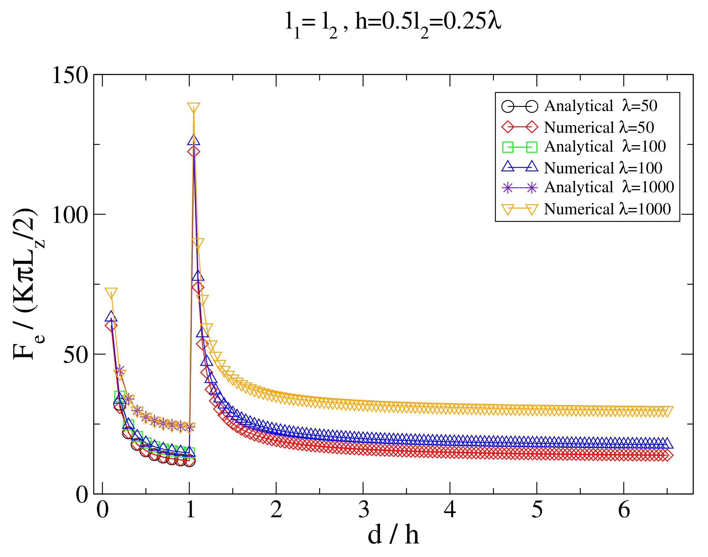
For a given substrate geometry and anchoring strength w, we have to obtain the value of d that minimizes Equation (5). As only depends on w and the set of nematic director singularities present in the texture, the value of d for a given interfacial state is determined by the surface and elastic contributions to the filled states. Furthermore, only the elastic contribution is relevant to obtain the value of d for the wet states. However, we found that in all cases the minimum free energy configuration for filled states (either or ) corresponds to , and for wetting states (either symmetric or asymmetric) to the limit. These observations can be rationalized by the fact that and, consequently, the surface term favors large values of d in the filled states. On the other hand, the higher the confinement of the nematic is, the larger the elastic distortions are and, consequently, the elastic free energy increases with the confinement. As an example, Figure 3 shows the decay of the elastic contribution to the free energy per substrate period and unit length along the z axis as a function of d for the asymmetric states ( if , otherwise). It is also clear in this figure that the numerical results for the elastic free energy of the state are in excellent agreement with the analytical expression Equation (A8) (with h replaced by d), and thus we used the latter for the calculations in this study. On the other hand, the limiting elastic free energy for the state at large d is given by the elastic free energy of a bulk nematic with the corresponding asymmetric texture in contact with the substrate [23], even when the angular field away from the substrate does not match the anchoring condition at the nematic–isotropic interface. This is due to the fact that the angular profile at large d and well above the substrate is linear in y as in a slit pore with an effective thickness , with a constant. Thus, the elastic free energy is inversely proportional to the effective thickness and, consequently, vanishes as .
We now proceed to calculate the interfacial phase diagram. To make contact with the previous Landau–de Gennes results [40], we consider substrates with , and . We start with large values of the substrate period , where the elastic and singularity cores contributions to the free energy are expected to be negligible with respect to . Under this assumption, we find that the D state is the most stable at small w, the F state is most stable at intermediate w and the W state is the most stable state at large w, irrespective of the substrate geometry. The phase boundary between the D and F states can be obtained by equating the surface free energies of both states, leading to the condition
which corresponds to the prediction of Wenzel’s law Equation (2) for . This approximation is valid for small w [37]. By contrast, the wetting transition between the F and the W states occurs exactly at the same value of w as for the planar case . We note that the phase boundaries depend on w and , but not on . Thus, we represent the phase diagrams in the representation.
This large-scale approximation does not distinguish between the F or W states with different nematic textures. However, as shown in Reference [23], the free energy difference between the and is due exclusively to . In addition, for the intermediate values of w that are relevant, is the most stable state at small h, while is the most stable state at large h. The phase boundary between the and states depends on w, and , and it is independent of the substrate period . Regarding the F states, the next-to-leading order contribution to the free energy is the logarithmic term of which arises from the director singularities. Equations (A8) and (A11) in Appendix B show that, for large , the logarithmic term of the state is twice that of the state. Thus, at large , only the states are stable.
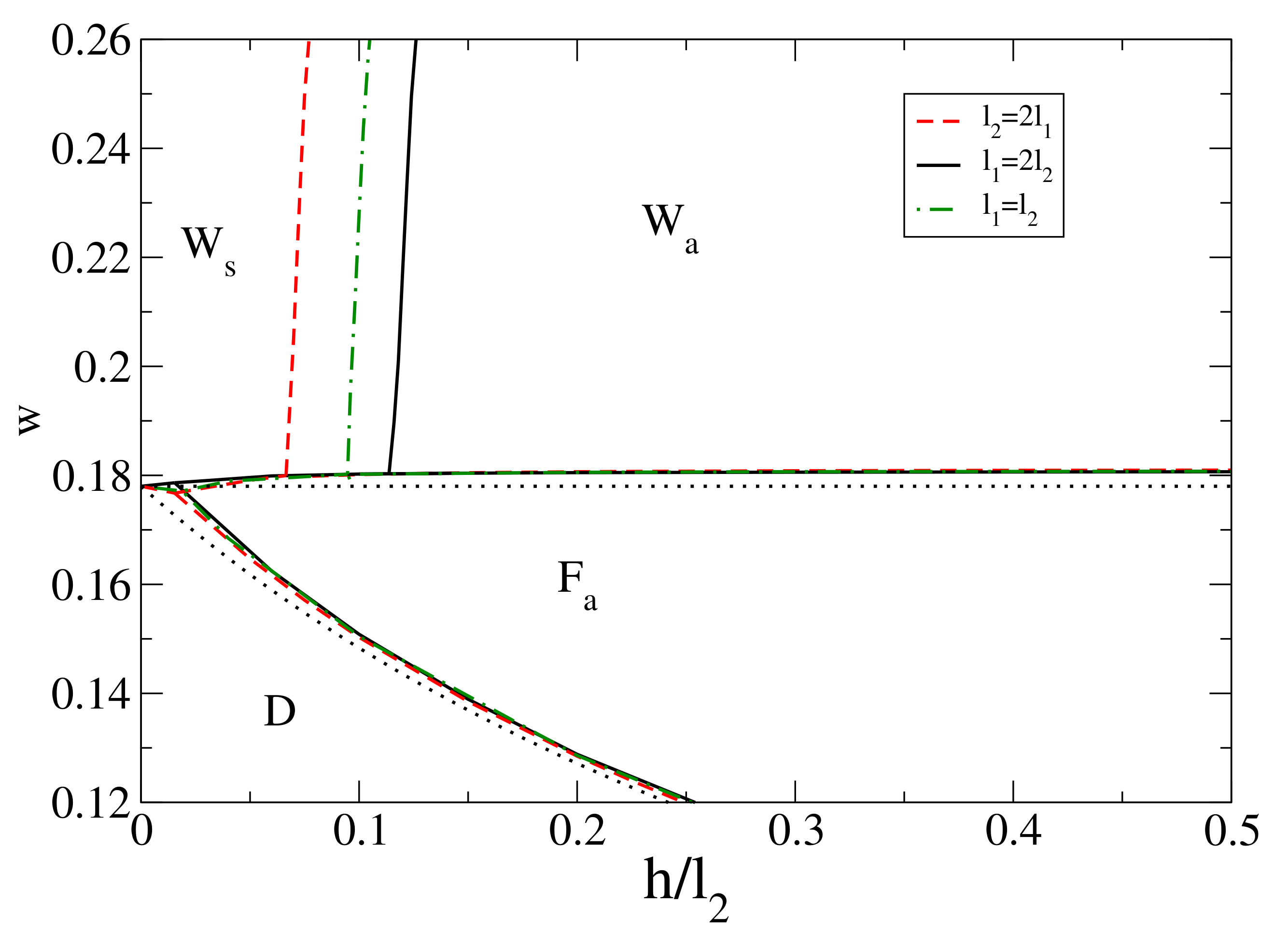
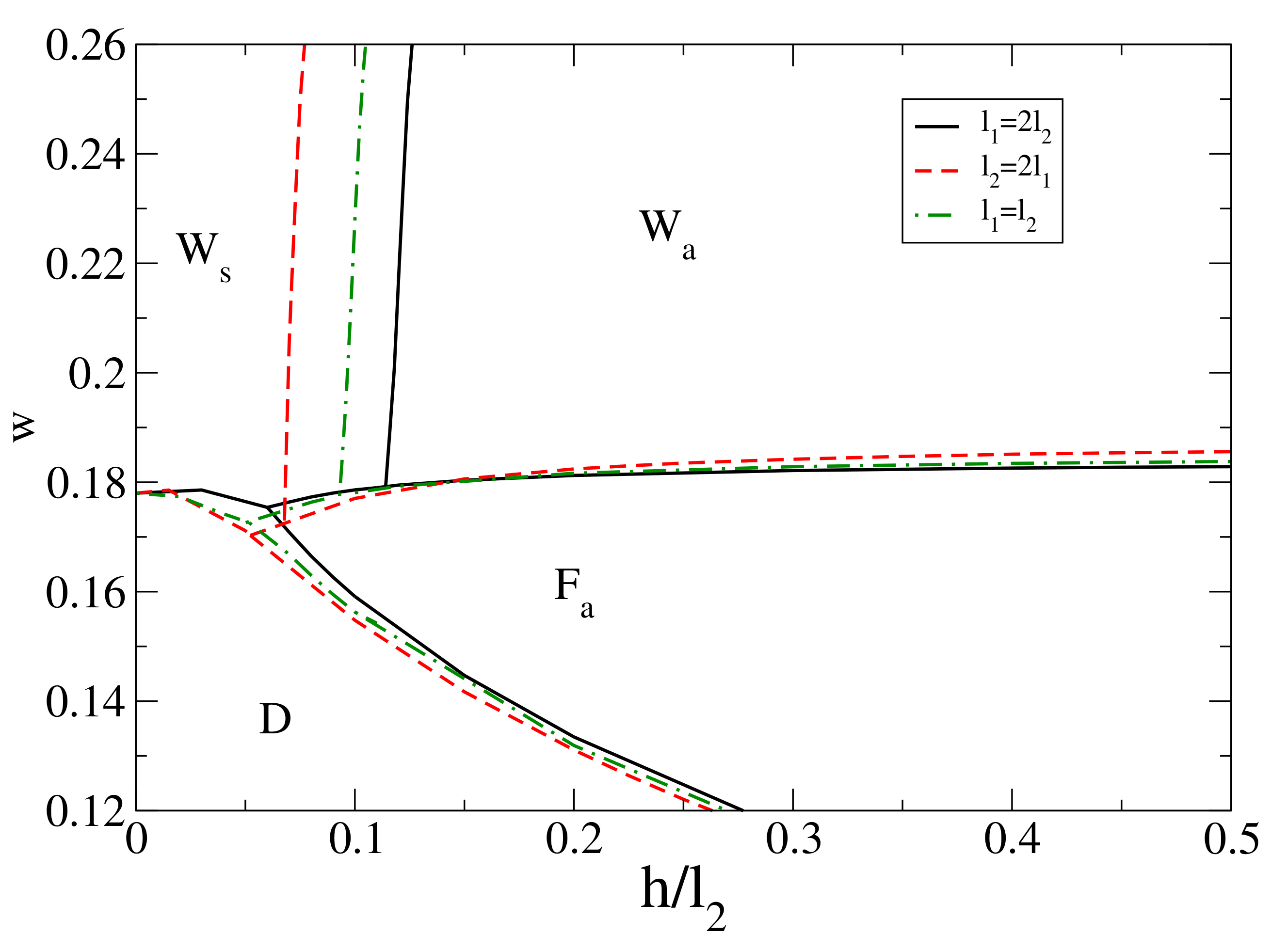
Figure 4 depicts the interfacial phase diagram for . First, we note that it is very similar to the phase diagram of the infinite period substrate, , considered previously. In addition, the phase boundaries are quite insensitive to the value of , with the exception of the boundary, which shifts to the left as decreases. The most distinctive features with respect to the case, are the emergence of a wetting transition at small and the increase of w at the wetting transition above , although it seems to saturate when . The existence of an asymptotic limit for large is not unexpected, and may be rationalized by the fact that the nematic texture deep in the groove becomes independent of h and resembles that of a bulk nematic in a rectangular well [23]. Thus, the elastic and defect free energy contributions of the distortions and singularities of this region of the groove will be the same in the and states and, consequently, a change in h will not affect the wetting transition. If is decreased to , the deviations with respect to the phase diagram increase (see Figure 5). We note that the relative stability of the D state with respect to the state is increased (the larger the ratio is, the more stable the D state becomes). On the other hand, the phase boundary moves to higher values of w, with a shift that increases with decreasing . However, the topology of the phase diagram is unchanged.
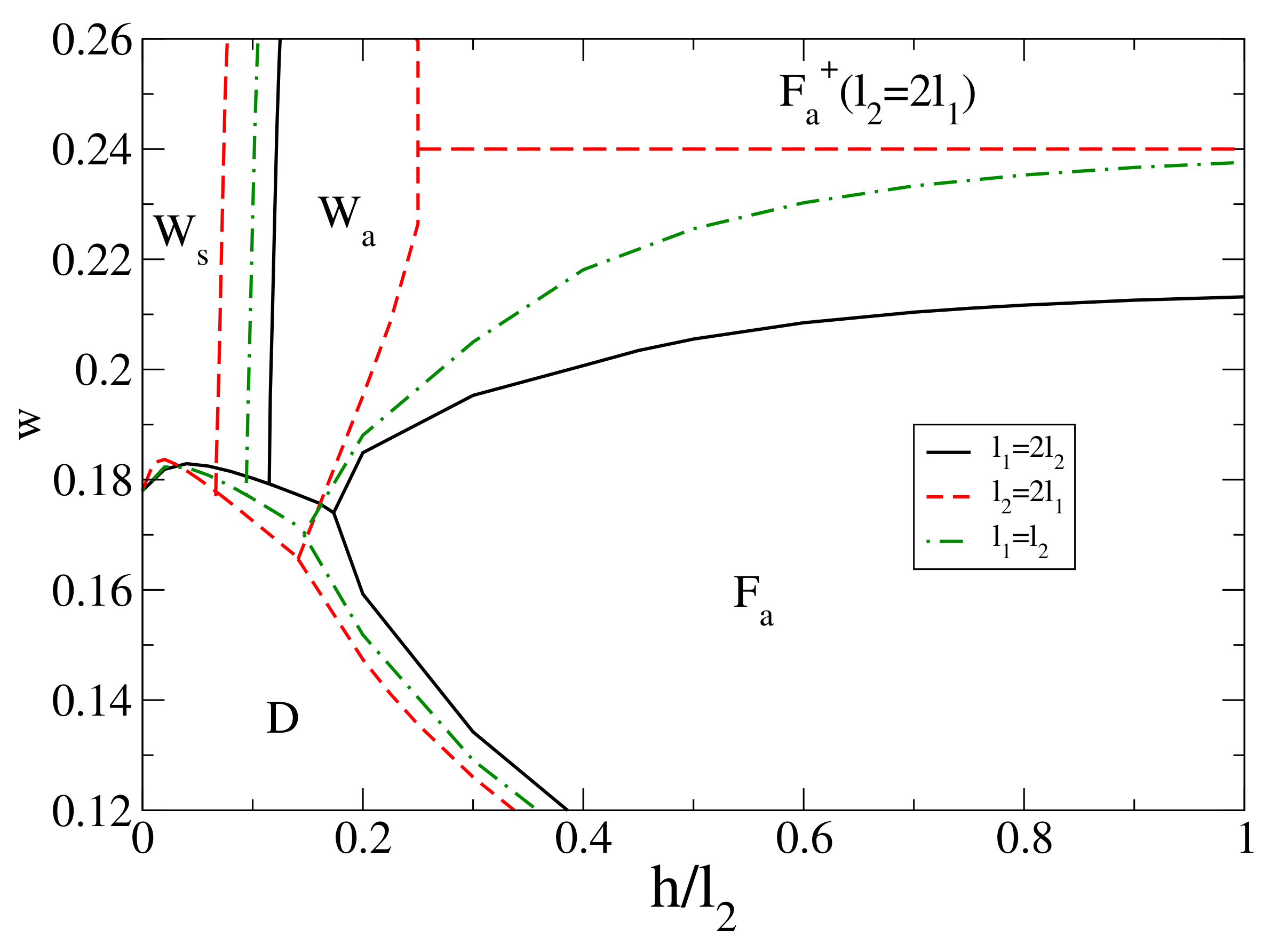
If we decrease the value of further, dramatic changes are observed in the phase diagram. As an example, Figure 6 shows the interfacial phase diagram for . As a first observation the shift of the phase boundary to larger values of leads to the disappearance of the coexistence between the and states and the emergence of a phase boundary. The most striking feature, however, is observed at the wetting transition. At and 2, the phase boundary shifts towards much larger values of w (larger for than for ), reaching the asymptotic value at higher values of than for the higher values of . Finally, at , we see a major change in the topology of the phase diagram: the state is suppressed at large , being replaced by states. Thus, the phase boundary becomes almost vertical. For the isotropic-substrate configuration changes from a microscopic thin paranematic layer to a configuration in which a microscopically thick layer of homeotropically-oriented nematic phase intrudes between the substrate and the bulk isotropic liquid phase. This is similar to the states in Reference [40], where a nematic droplet phase nucleates on the upper surface of the substrate. By analogy, we denote this state by .
The suppression of the wetting states at large was also reported for the Landau–de Gennes theory in Reference [40]. For small , the elastic and core contributions to the free energy, which favor the state, are lower than the difference between the top substrate surface contributions between and . This also explains why this is first observed at small values of .
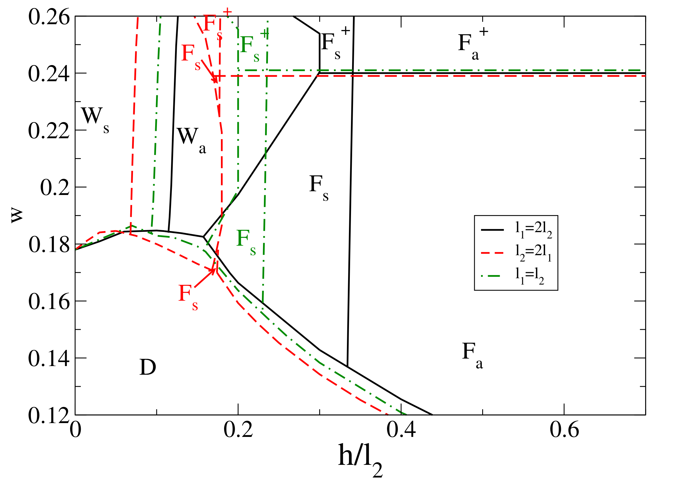
As is further reduced, the suppression of the wetting states at large is extended to larger values of . Furthermore, new features appear in the phase diagram. Figure 7 illustrates the interfacial phase diagram for . At intermediate values of , the state is suppressed in favor of the state, indicating that the difference between core contributions to the free energy in the filled states, which favors the state, overcomes the difference of the logarithmic contributions in which favors the state. As for the asymmetric filled states at large , we can distinguish between and depending on w, being smaller or larger than , the value above which a thick layer of nematic is formed on the top substrate surface. However, at this length scale, the nematic texture differs from that depicted in Figure 2a. As described in Appendix A, the isotropic–nematic interface exhibits a significant distortion near the disclination core. Thus, the microscopic length scale associated to the interfacial deformation, which is of order 10, becomes comparable to h (note that appears for h in the range 40–60). As a result, the true interfacial configuration of the symmetric filled states resembles that of the and states reported in Reference [40]. As a conclusion, the topology of the phase diagram for starts to exhibit features similar to those of the small period substrates reported for the Landau–de Gennes theory.
4. Discussion and Conclusions
We studied the interfacial phase diagram of a bulk isotropic liquid in contact with a crenellated substrate which favors the nematic with homeotropic anchoring. This study was based on the modified Frank–Oseen formalism, which separates surface, elastic and singularity cores contributions. We selected parameters in line with those of the Landau–de Gennes theory reported in Reference [40] to facilitate the comparison between the two approaches. First, we identified the relevant interfacial states and their features. We found that, in addition to the dry D state, there are two filled states and and two wet states and characterized by different nematic textures. The different contributions to the free energy were evaluated either numerically or analytically. We calculated the interfacial phase diagram in terms of the anchoring strength w and the grooves depth-to-width aspect ratio for values of the periodicity ranging from 500 to bulk correlation lengths. For large values of and , we obtained a phase diagram with a topology similar to that of simple fluids. In general, wetting of a substrate with a given geometry occurs in two steps as w increases: first from a dry to an asymmetric filled state, and then to a completely wet state. A direct transition from dry to a completely wet state is observed only for very shallow substrates. Furthermore, the rougher the substrate is, the lower the value of w at the transition. Finally, the completely wet state exhibits symmetric textures for shallow substrates, and asymmetric ones otherwise.
As decreases to , we observed significant changes in the topology of the phase diagram, in particular the suppression of the completely wet state and its substitution by a filled state for rough substrates and large w. This result is at odds with the expectation, based on Wenzel’s law [33], that the roughness of hydrophilic substrates favors wetting. This feature is more prominent as is decreased to 500 and, in addition, the state is stabilized for intermediate values of . This is one order of magnitude larger than the largest considered in the Landau–de Gennes study of Reference [40], but we observed the same qualitative features of the phase diagrams reported there.
We may be tempted to push the calculations reported here to lower values of , but it is clear that is already at limit of validity of the modified Frank–Oseen approach, which is based on the separation of length scales, which determine distinct additive contributions to the free energy [22]. While surface contributions are determined by the order parameter profiles, which vary in the range of a few correlation lengths around the substrate or at the interface, the elastic contribution assumes that the nematic tensor is bulk-like in most of the nematic region. Finally, the presence of triple isotropic–nematic–substrate or disclination lines at the isotropic–nematic interface introduces new microscopic length scales of the order of tens of correlation lengths in filled F states, as shown in Appendix A. Thus, our approximation will breakdown for smaller values of (especially in the regions involving F states) and our predictions will not be reliable.
Author Contributions
Conceptualization and supervision, J.M.R.-E. and M.M.T.d.G.; investigation, software, and data curation, Ó.A.R.-G. and J.M.R.-E.; and writing, Ó.A.R.-G., J.M.R.-E. and M.M.T.d.G.
Funding
This research was funded by Ministerio de Economía y Competitividad (Spain) grant number FIS2017-87117-P and the Portuguese Foundation for Science and Technology (FCT) under the contracts: PTDC/FISMAC/28146/2017 (LISBOA-01-0145-FEDER-028146) and UID/FIS/00618/2019. M.M.T.G. would like to thank the Isaac Newton Institute for Mathematical Sciences for support and hospitality during the program “The mathematical design of new materials”. This program was supported by EP-SRC Grant Number: EP/R014604/1. Her participation in the program was supported in part by a Simons Foundation Fellowship.
Conflicts of Interest
The authors declare no conflict of interest.
Appendix A. Evaluation of
In this appendix, we summarize the methodology to obtain the disclinations and singularities core contributions within the Landau–de Gennes theory. The value of is the sum of the contributions arising from each isolated singularity. As mentioned previously, the procedure to obtain the core contribution of each singularity is based on a full minimization of the Landau–de Gennes theory by using an adaptive-meshing finite-element method combined with a conjugate-gradient minimization algorithm [50]. The symmetry of the problem allows the solution to be obtained in a 2D domain with shape and boundary conditions specific for each type of singularity.
Appendix A.1. Substrate Corner Singularity
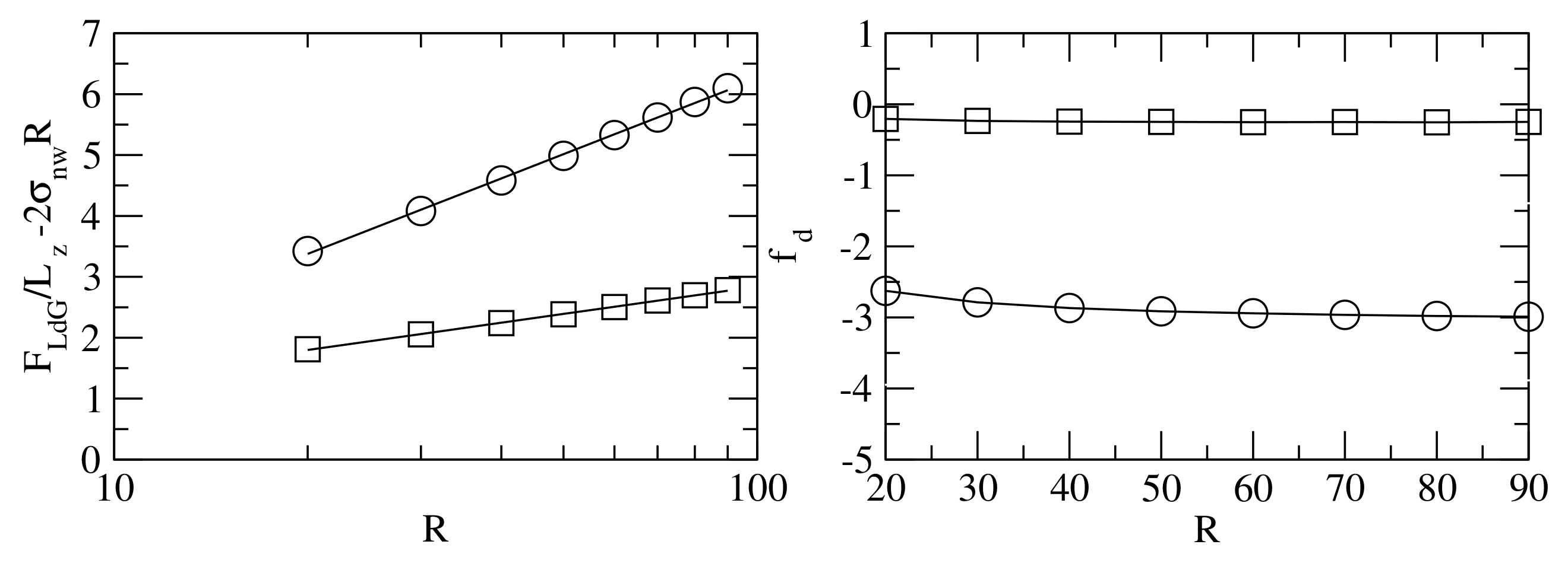
In both filled and wet states, nematic director singularities appear close to the substrate corners, with topological charges for the bottom corners, and for the top corners. We follow the procedure described in Ref. [22] to evaluate the core contributions to the free energy. The domain considered is a circular sector of radius R and opening angle either equal to (bottom corners) or to (top corners). On the straight boundaries, we do not fix the nematic ordering tensor, but we use the surface contribution (Equation (9)). On the circular boundary, Dirichlet boundary conditions on are applied, where the nematic order parameter S takes the value of the planar substrate order-parameter profile, taking as the distance between the boundary and the substrate that to the closest wall. The biaxiality parameter B is assumed to vanish everywhere on the boundary. Finally, the angular field is given by , where is the polar angular coordinate of the point at the boundary and I is the topological charge of the corner singularity. We calculate the equilibrium free energies for different values of R, and fit the results to the expression
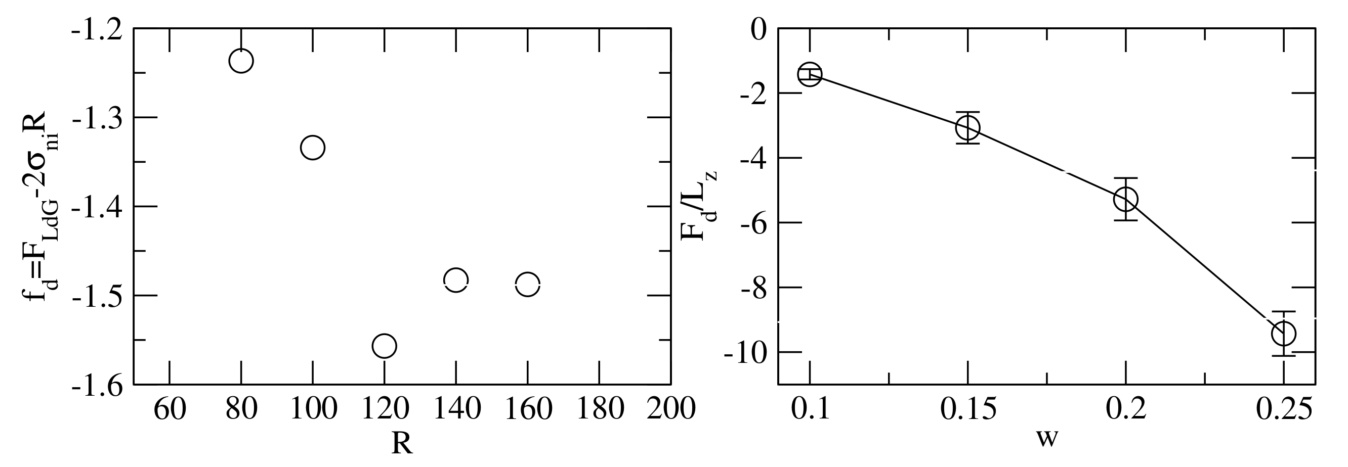
where , is the substrate length along the z axis and is the nematic correlation length. Figure A1 shows that, when the surface contribution is subtracted, the free energy follows a logarithmic dependence on R. If we further subtract the logarithmic term from Equation (A1), we find that still shows a slight dependence on R, but it seems to converge to a well-defined value for , which we identify as . The dependence of on w is reported in Figure 9 of Reference [23].
Figure A1.
(Left) Plot of as a function of R for . Configurations with opening angle and topological charge are depicted by circles and configurations with opening angle and topological charge depicted by squares. (Right) Plot of as a function of R. The meaning of the symbols is the same as in the left panel.

Appendix A.2. Disclination Line on the Nematic–Isotropic Interface
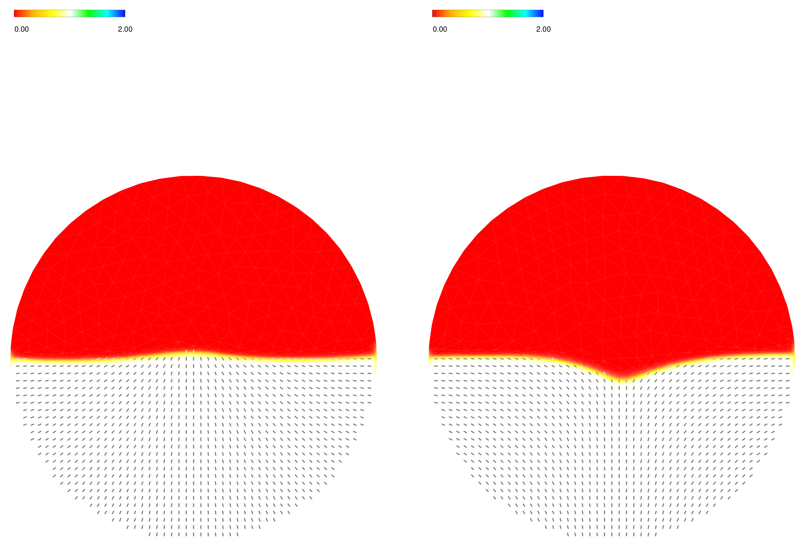
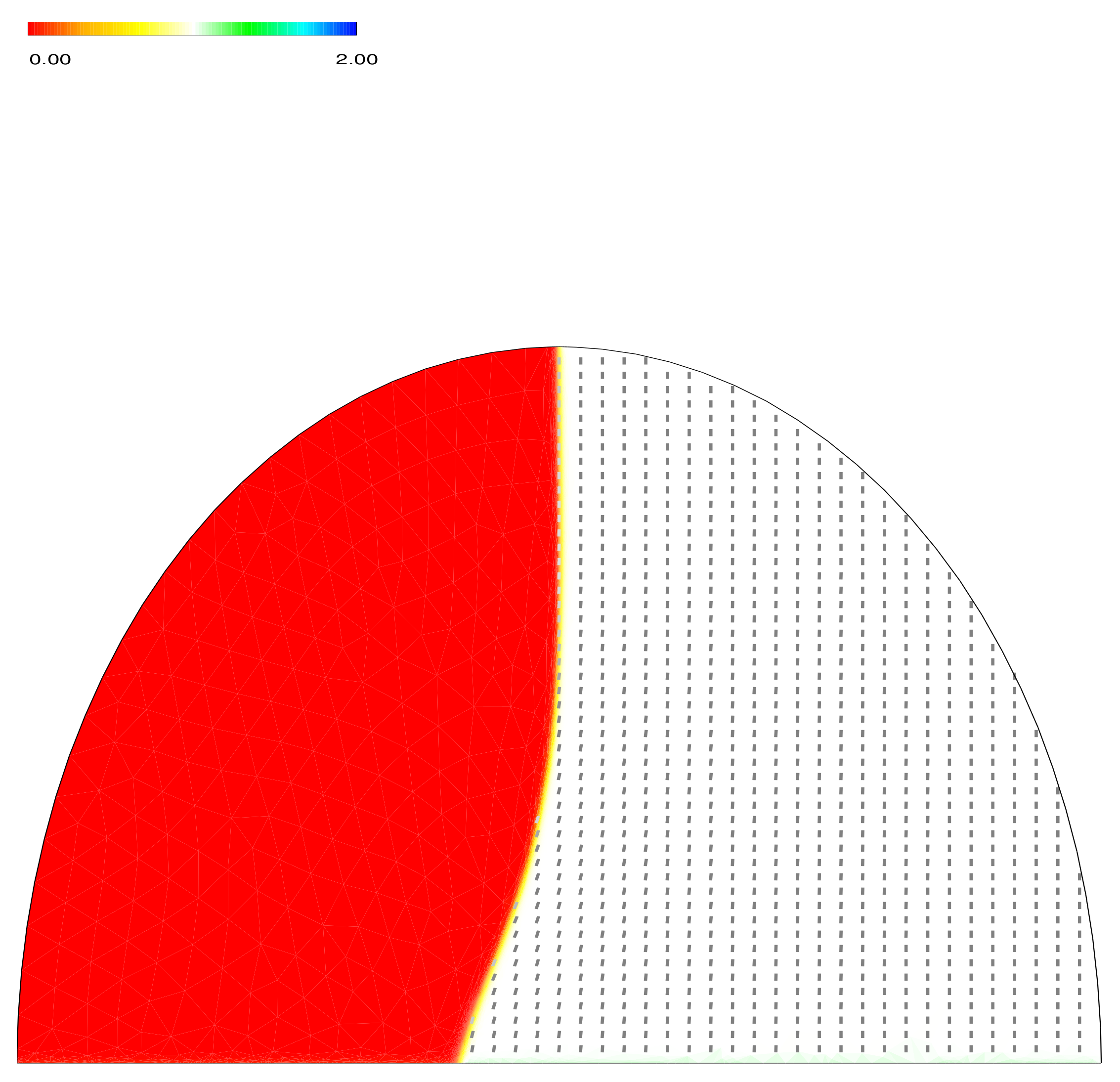
Next, we evaluate the free-energy contribution of a disclination line on the nematic–isotropic interface. This defect appears in the configuration with a topological charge , but in general the topological charge I can be either or . In this case, the geometry considered for the minimization of the Landau–de Gennes theory is a circle of radius R. Dirichlet boundary conditions on are used in a way similar to the substrate corner singularity: the nematic order parameter S and biaxiality parameter B along the boundary are taken from the profiles of a nematic–isotropic free interface located on the x axis, and the angular field obeys . Typical profiles are shown in Figure A2. We find that a disclination singularity is nucleated near the center of the circle. Furthermore, its presence distorts the nematic–isotropic interface. Typically, for large R this deformation has a nearly Gaussian shape, with a root-mean-square width of about and a height of about . These large deviations introduce a new length scale in the problem, so our modified Frank–Oseen model is expected to be valid when the substrate relief length scales are much larger.
Figure A2.
Nematic order parameter (color code) and nematic director (segments) of a nematic–isotropic interfacial configuration with a disclination line of topological charge (left) and (right), for .
Figure A2.
Nematic order parameter (color code) and nematic director (segments) of a nematic–isotropic interfacial configuration with a disclination line of topological charge (left) and (right), for .

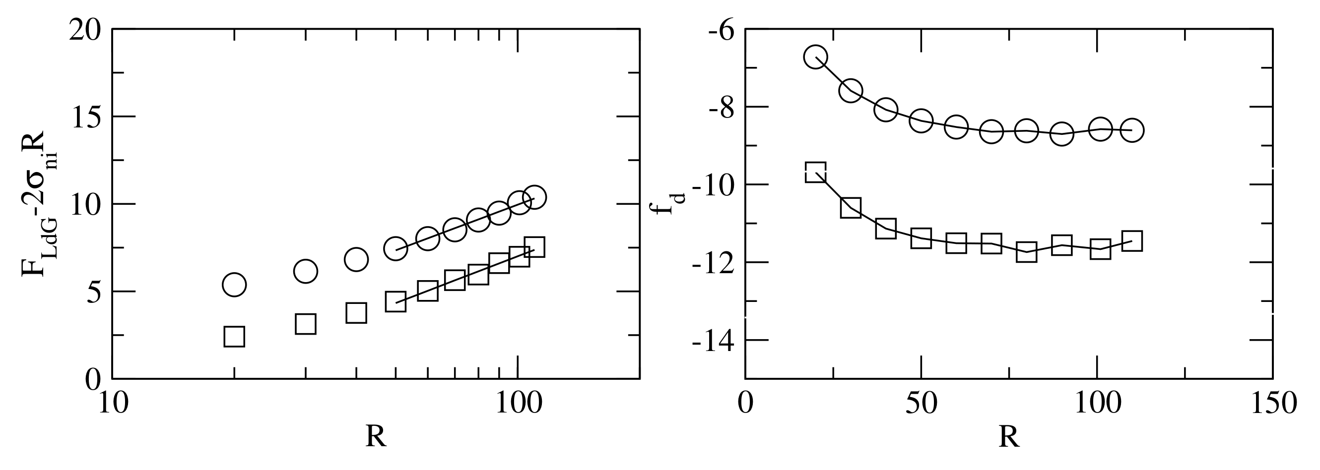
To estimate the free-energy contribution of the disclination, we calculate the equilibrium free energies for different values of R and we fit the results to the expression
in a way similar to the previous case. Figure A3 shows that the convergence of occurs at larger values of R when compared to the substrate corner singularity, in agreement with the emergence of the new microscopic length scale.
Figure A3.
(Left) Plot of as a function of R for interfacial nematic–isotropic configurations with a disclination line of topological charge (circles) and a disclination line of topological charge (squares). (Right) Plot of as a function of R. The meaning of the symbols is the same as in the left panel.

Appendix A.3. Line Tension of the Substrate–Isotropic–Nematic Contact Line
Finally, the F states exhibit a contact line between the substrate and the nematic–isotropic interface. There is no singularity in the nematic director associated to this contact line, but there is a line tension contribution that can be estimated in a similar way. Here, the domain is a half a circle. On the horizontal straight boundary, we do not fix the nematic ordering tensor, but we use the surface contribution Equation (9). On the circular boundary we impose Dirichlet boundary conditions, which depend on the horizontal coordinate x: if , satisfies the order parameter nematic-substrate profile, while if , satisfies the order parameter isotropic-substrate profile. Finally, for , is the order parameter profile associated to a nematic–isotropic interface located on the y axis. A typical configuration is shown in Figure A4. We also observe the deformation of the nematic–isotropic interface close to the substrate, in particular when the wetting transition is approached.
To estimate the free-energy contribution of the disclination, we calculate the equilibrium free energies for different values of R and we fit the results to the expression
It is seen in Figure A5 that the values of fluctuate more than in the previous cases, but we can average them to obtain an estimate of both and the error. Its dependence on w is also shown.
Figure A4.
Plot of the nematic order parameter (color code) and nematic director (segments) of a nematic–isotropic interfacial configuration in contact with a substrate with anchoring strength and .
Figure A4.
Plot of the nematic order parameter (color code) and nematic director (segments) of a nematic–isotropic interfacial configuration in contact with a substrate with anchoring strength and .

Figure A5.
(Left) Plot of as a function of R for interfacial nematic–isotropic configurations in contact with a substrate with anchoring strength . (Right) Plot of as a function of w.
Figure A5.
(Left) Plot of as a function of R for interfacial nematic–isotropic configurations in contact with a substrate with anchoring strength . (Right) Plot of as a function of w.

Appendix B. Exact Evaluation of for States
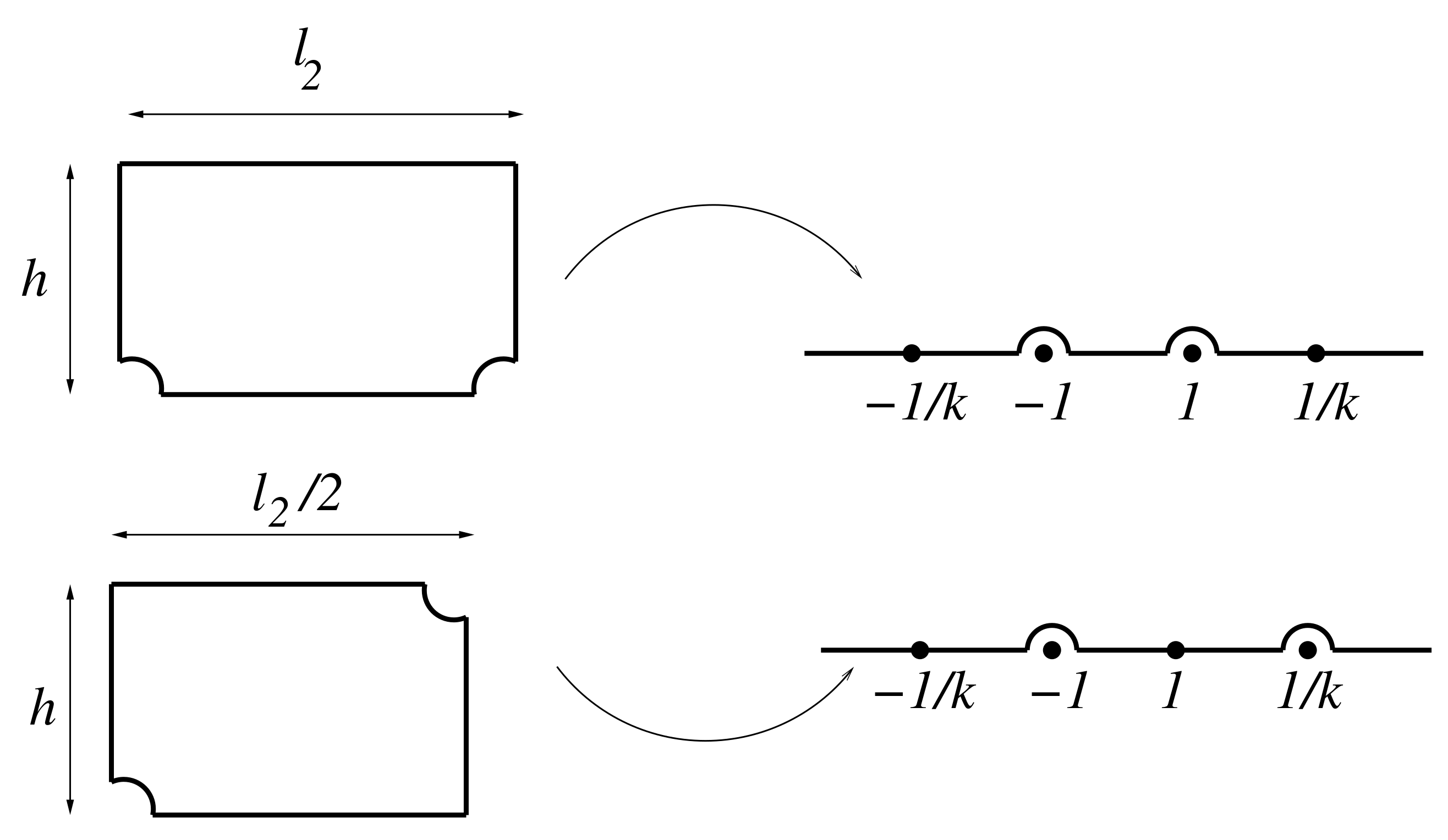
In this appendix, we evaluate the elastic contribution of the and states by using the Schwarz–Christoffel conformal mapping technique. For the asymmetric state , we use the full nematic phase domain, which is a rectangle of width and height h. The domain is rounded around the bottom corners by arcs of circle of radii in order to avoid the director singularity associated to the corners (see Figure A6). For the asymmetric state, the boundary conditions are along the bottom horizontal side, and on the other sides. The Schwarz–Christoffel transformation
maps the interior of the rectangle in the upper half complex plane, with the upper corners mapped onto the positions and the lower corners onto . In this expression, F is the incomplete elliptic integral of the first kind. These conditions fix the values of C and . Furthermore, the parameter k can be related to the aspect ratio of the rectangle. After some algebra, it can be shown that
where and are, respectively, the real and imaginary parts of the complex number z.
Figure A6.
Schematic picture of the Schwarz–Christoffel transformation to obtain the elastic contribution to the free energy of the state (upper rectangle) and the state (lower rectangle).
Figure A6.
Schematic picture of the Schwarz–Christoffel transformation to obtain the elastic contribution to the free energy of the state (upper rectangle) and the state (lower rectangle).

In the plane, the Laplace equation in the upper half complex plane with boundary conditions for and for and has as solution
where and is the radius of the transformed arc which avoids the singularities at given by
Now, we can evaluate as
where is the surface length along the z axis. The first contribution is the singular part associated with the director singularities which appear close to the bottom corners, and the second contribution depends only on the aspect ratio .
For the state, we transform half the nematic domain to the upper half complex plane (see Figure A6). The rectangle is now rounded around the left bottom and right upper corners, and the boundary conditions are for the upper and left sides and for the lower and right sides. The transformation is still given by Equation (A4), but Equation (A5) is valid if is replaced by . Now, the Laplace equation on the upper half complex plane with boundary conditions for and for and has as solution
where and are the radii of the transformed arcs which avoid the singularities at and , respectively, with expressions
Now, we obtain as previously
Again, the first contribution is the singular part associated with the director singularities close to the corners and on the nematic–isotropic interface, and the second contribution depends only on the aspect ratio .
References
- Lee, B.-W.; Clark, N.A. Alignment of Liquid Crystals with Patterned Isotropic Surfaces. Science 2001, 291, 2576–2580. [Google Scholar] [CrossRef] [PubMed]
- Kim, J.-H.; Yoneya, M.; Yokoyama, H. Tristable nematic liquid-crystal device using micropatterned surface alignment. Nature 2002, 420, 159–162. [Google Scholar] [CrossRef] [PubMed]
- Ferjani, S.; Choi, Y.; Pendery, J.; Petschek, R.G.; Rosenblatt, C. Mechanically Generated Surface Chirality at the Nanoscale. Phys. Rev. Lett. 2010, 104, 257801. [Google Scholar] [CrossRef] [PubMed]
- Brown, C.V.; Towler, M.J.; Hui, V.C.; Bryan-Brown, G.P. Numerical analysis of nematic liquid crystal alignment on asymmetric surface grating structures. Liq. Cryst. 2000, 27, 233–242. [Google Scholar] [CrossRef]
- Uche, C.; Elston, S.J.; Parry-Jones, L.A. Microscopic observation of zenithal bistable switching in nematic devices with different surface relief structures. J. Phys. D Appl. Phys. 2005, 38, 2283–2291. [Google Scholar] [CrossRef]
- Uche, C.; Elston, S.J.; Parry-Jones, L.A. Modelling zenithal bistability at an isolated edge in nematic liquid crystal cells. Liq. Cryst. 2006, 33, 697–704. [Google Scholar] [CrossRef]
- Davidson, A.J.; Brown, C.V.; Mottram, N.J.; Ladak, S.; Evans, C.R. Defect trajectories and domain-wall loop dynamics during two-frequency switching in a bistable azimuthal nematic device. Phys. Rev. E 2010, 81, 051712. [Google Scholar] [CrossRef]
- Evans, C.R.; Davidson, A.J.; Brown, C.V.; Mottram, N.J. Static alignment states in a bistable azimuthal nematic device with blazed grating sidewalls. J. Phys. D: Appl. Phys. 2010, 43, 495105. [Google Scholar] [CrossRef]
- Dammone, O.J.; Zacharoudiou, I.; Dullens, R.P.A.; Yeomans, J.M.; Lettinga, M.P.; Aarts, D.G.A.L. Confinement Induced Splay-to-Bend Transition of Colloidal Rods. Phys. Rev. Lett. 2012, 109, 108303. [Google Scholar] [CrossRef] [Green Version]
- Silvestre, N.M.; Patrício, P.; da Gama, M.M.T. Key-lock mechanism in nematic colloidal dispersions. Phys. Rev. E 2004, 69, 061402. [Google Scholar] [CrossRef] [Green Version]
- Ohzono, T.; Fukuda, J.-I. Zigzag line defects and manipulation of colloids in a nematic liquid crystal in microwrinkle grooves. Nat. Commun. 2012, 3, 701. [Google Scholar] [CrossRef] [PubMed]
- Sengupta, A.; Bahr, C.; Herminghaus, S. Topological microfluidics for flexible micro-cargo concepts. Soft Matter. 2013, 9, 7251–7260. [Google Scholar] [CrossRef] [Green Version]
- Lavrentovich, O.D. Transport of particles in liquid crystals. Soft Matter. 2014, 10, 1264–1283. [Google Scholar] [CrossRef] [PubMed]
- Luo, Y.; Serra, F.; Beller, D.A.; Gharbi, M.A.; Li, N.; Yang, S.; Kamien, R.D.; Stebe, K.J. Around the corner: Colloidal assembly and wiring in groovy nematic cells. Phys. Rev. E 2016, 93, 032705. [Google Scholar] [CrossRef]
- Luo, Y.; Serra, F.; Stebe, K.J. Experimental realization of the “lock-and-key” mechanism in liquid crystals. Soft Matter 2016, 12, 6027–6032. [Google Scholar] [CrossRef] [PubMed]
- Luo, Y.; Beller, D.A.; Bionello, G.; Serra, F.; Stebe, K.J. Tunable colloid trajectories in nematic liquid crystals near wavy walls. Nat. Commun. 2018, 9, 3841. [Google Scholar] [CrossRef]
- Barbero, G. Surface geometry and induced orientation of a nematic liquid crystal. Lett. Nuovo Cimento Soc. Ital. Fis. 1980, 29, 553–559. [Google Scholar] [CrossRef]
- Barbero, G. On the critical angle of a NLC cell. Lett. Nuovo Cimento Soc. Ital. Fis. 1981, 32, 60–64. [Google Scholar] [CrossRef]
- Barbero, G.; Scaramuzza, N. On the interface substrate-nematic: Anchoring energy and topography. Lett. Nuovo Cimento Soc. Ital. Fis. 1982, 34, 173–179. [Google Scholar] [CrossRef]
- Poniewierski, A. Nematic liquid crystal in the wedge and edge geometry in the case of homeotropic alignment. Eur. Phys. J. E 2010, 31, 169–178. [Google Scholar] [CrossRef]
- Romero-Enrique, J.M.; Pham, C.-T.; Patrício, P. Scaling of the elastic contribution to the surface free energy of a nematic liquid crystal on a sawtoothed substrate. Phys. Rev. E 2010, 82, 011707. [Google Scholar] [CrossRef] [Green Version]
- Rojas, O.A.; Romero-Enrique, J.M. Generalized Berreman’s model of the elastic surface free energy of a nematic liquid crystal on a sawtoothed substrate. Phys. Rev. E 2012, 86, 041706. [Google Scholar] [CrossRef]
- Rojas, O.A.; Romero-Enrique, J.M.; Silvestre, N.M.; da Gama, M.M.T. Pattern-induced anchoring transitions in nematic liquid crystals. J. Phys. Condens. Matter. 2017, 29, 064002. [Google Scholar]
- Harnau, L.; Penna, F.; Dietrich, S. Colloidal hard-rod fluids near geometrically structured substrates. Phys. Rev. E 2004, 70, 021505. [Google Scholar] [CrossRef] [Green Version]
- Bramble, J.P.; Evans, S.D.; Henderson, J.R.; Anquetil, C.; Cleaver, D.J.; Smith, N.J. Nematic liquid crystal alignment on chemical patterns. Liq. Cryst. 2007, 34, 1059–1069. [Google Scholar] [CrossRef] [Green Version]
- Sheng, P. Boundary-layer phase transition in nematic liquid crystals. Phys. Rev. A 1982, 26, 1610–1617. [Google Scholar] [CrossRef] [Green Version]
- Braun, F.N.; Sluckin, T.J.; Velasco, E. Director distortion in a nematic wetting layer. J. Phys. Condens. Matter 1996, 8, 2741–2754. [Google Scholar] [CrossRef]
- Yokoyama, H.; Kobayashi, S.; Kamei, H. Boundary Dependence of the Formation of New Phase at the Isotropic-Nematic Transition. Mol. Cryst. Liq. Cryst. 1983, 99, 39–52. [Google Scholar] [CrossRef]
- Hsiung, H.; Rasing, T.; Shen, Y.R. Wall-Induced Orientational Order of a Liquid Crystal in the Isotropic Phase–an Evanescent-Wave-Ellipsometry Study. Phys. Rev. Lett. 1986, 57, 3065–3068. [Google Scholar] [CrossRef]
- Hsiung, H.; Rasing, T.; Shen, Y.R. Erratum to “Wall-Induced Orientational Order of a Liquid Crystal in the Isotropic Phase–an Evanescent-Wave-Ellipsometry Study”. Phys. Rev. Lett. 1987, 59, 1983. [Google Scholar] [CrossRef]
- Chen, W.; Martinez-Miranda, L.J.; Hsiung, H.; Shen, Y.R. Orientational wetting behavior of a liquid-crystal homologous series. Phys. Rev. Lett. 1989, 62, 1860–1863. [Google Scholar] [CrossRef]
- Alkhairalla, B.; Allinson, H.; Boden, N.; Evans, S.D.; Henderson, J.R. Anchoring and orientational wetting of nematic liquid crystals on self-assembled monolayer substrates: An evanescent wave ellipsometric study. Phys. Rev. E 1999, 59, 3033–3039. [Google Scholar] [CrossRef]
- Quéré, D. Wetting and Roughness. Ann. Rev. Mater. Res. 2008, 38, 71–99. [Google Scholar] [CrossRef]
- Rascón, C.; Parry, A.O.; Sartori, A. Wetting at nonplanar substrates: Unbending and unbinding. Phys. Rev. E 1999, 59, 5697–5700. [Google Scholar] [CrossRef] [Green Version]
- Rascón, C.; Parry, A.O. Geometry-dominated fluid adsorption on sculpted solid substrates. Nature (London) 2000, 407, 986–989. [Google Scholar] [CrossRef] [Green Version]
- Patrício, P.; Romero-Enrique, J.M.; Silvestre, N.M.; Bernardino, N.R.; da Gama, M.M.T. Complex fluids at complex surfaces: Simply complicated? Mol. Phys. 2011, 109, 1067–1075. [Google Scholar] [CrossRef]
- Patrício, P.; Pham, C.-T.; Romero-Enrique, J.M. Wetting Transition of a Nematic Liquid Crystal on a Periodic Wedge-Structured Substrate. Eur. Phys. J. E 2008, 26, 97–101. [Google Scholar] [CrossRef]
- Patrício, P.; Silvestre, N.M.; Pham, C.-T.; Romero-Enrique, J.M. Filling and wetting transitions of nematic liquid crystals on sinusoidal substrates. Phys. Rev. E 2011, 84, 021701. [Google Scholar] [CrossRef]
- Silvestre, N.M.; Romero-Enrique, J.M.; da Gama, M.M.T. Nematic liquid crystals on sinusoidal channels: The zigzag instability. J. Phys. Condens. Matter 2017, 29, 014004. [Google Scholar] [CrossRef]
- Silvestre, N.M.; Eskandari, Z.; Patrício, P.; Romero-Enrique, J.M.; da Gama, M.M.T. Nematic wetting and filling of crenellated surfaces. Phys. Rev. E 2012, 86, 011703. [Google Scholar] [CrossRef]
- Blow, M.L.; da Gama, M.M.T. Interfacial motion in flexo- and order-electric switching between nematic filled states. J. Phys. Condens. Matter 2013, 25, 245103. [Google Scholar] [CrossRef] [Green Version]
- de Gennes, P.-G.; Prost, J. The Physics of Liquid Crystals, 2nd ed.; Clarendon Press: Oxford, UK, 1995. [Google Scholar]
- Oseen, C.W. The theory of liquid crystals. Trans. Faraday Soc. 1933, 29, 883–898. [Google Scholar] [CrossRef]
- Frank, F.C. On the theory of liquid crystals. Discuss. Faraday Soc. 1958, 25, 19–28. [Google Scholar] [CrossRef]
- Davidson, A.J.; Mottram, N.J. Conformal mapping techniques for the modelling of liquid crystal devices. Eur. J. Appl. Math. 2012, 23, 99–119. [Google Scholar] [CrossRef]
- Ledney, M.F.; Tarnavskyy, O.S.; Lesiuk, A.I.; Reshetnyak, V.Y. Equilibrium configurations of director in a planar nematic cell with one spatially modulated surface. Condens. Matter Phys. 2016, 19, 33604. [Google Scholar] [CrossRef] [Green Version]
- Ledney, M.F.; Tarnavskyy, O.S.; Lesiuk, A.I.; Reshetnyak, V.Y. Modelling of director equilibrium states in a nematic cell with relief surface. Liq. Cryst. 2017, 44, 312–321. [Google Scholar] [CrossRef]
- Tarnavskyy, O.S.; Ledney, M.F.; Lesiuk, A.I. Generalised technique for calculation of plane director profiles in bounded nematic liquid crystals. Liq. Cryst. 2018, 45, 641–648. [Google Scholar] [CrossRef]
- Finotello, D.; Iannacchione, G.S.; Qian, S. Phase transitions in Restricted Geometries. In Liquid Crystals in Complex Geometries.; Crawford, G.P., Žumer, S., Eds.; Taylor&Francis: London, UK, 1996; pp. 325–344. [Google Scholar]
- Patrício, P.; Tasinkevych, M.; da Gama, M.M.T. Coloidal dipolar interactions in 2D smectic C films. Eur. Phys. J. E 2002, 7, 117–122. [Google Scholar] [CrossRef]
Figure 1.
Schematic picture of an interfacial configuration of a nematic layer of thickness d (in green) at coexistence with a bulk isotropic liquid (in white) on a crenellated substrate with depth h and length scales and . The nematic–isotropic interface and the director field in the nematic phase (in red) are also highlighted.

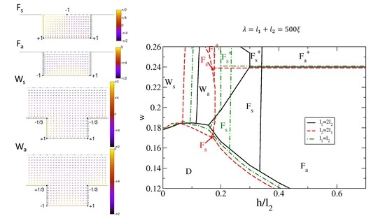
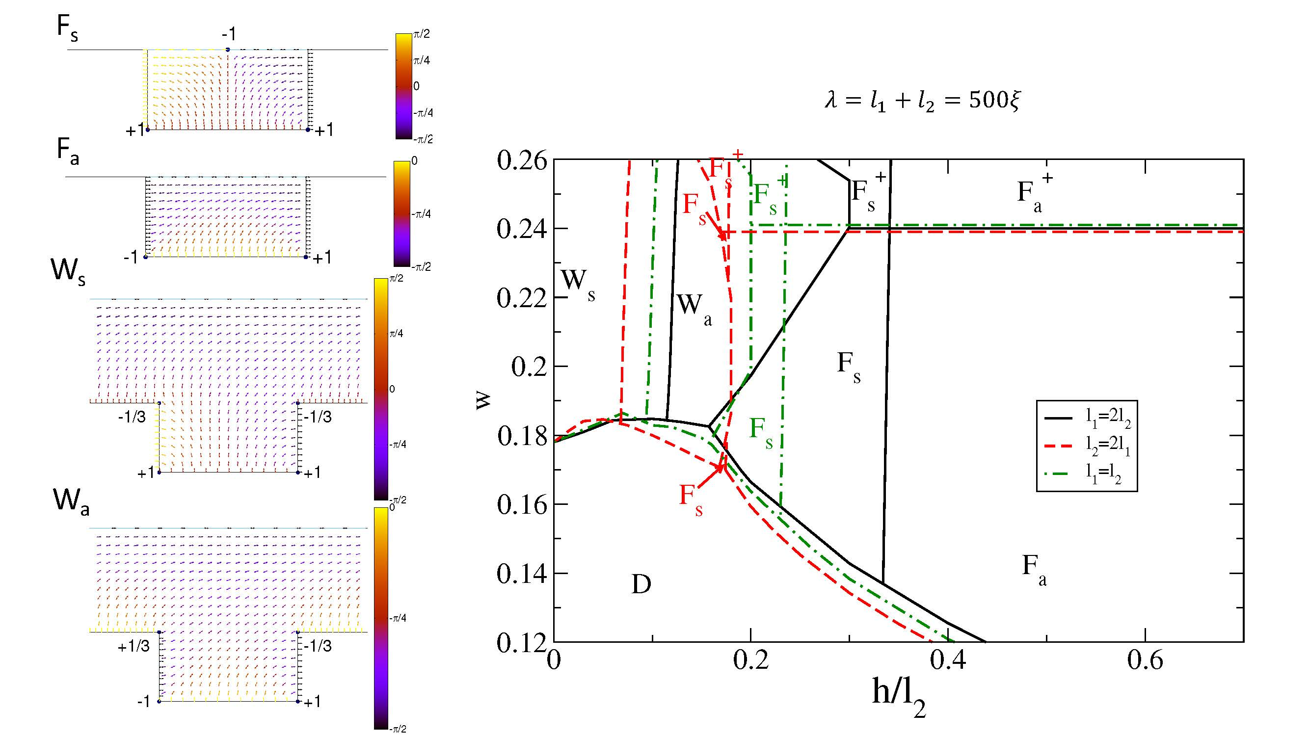
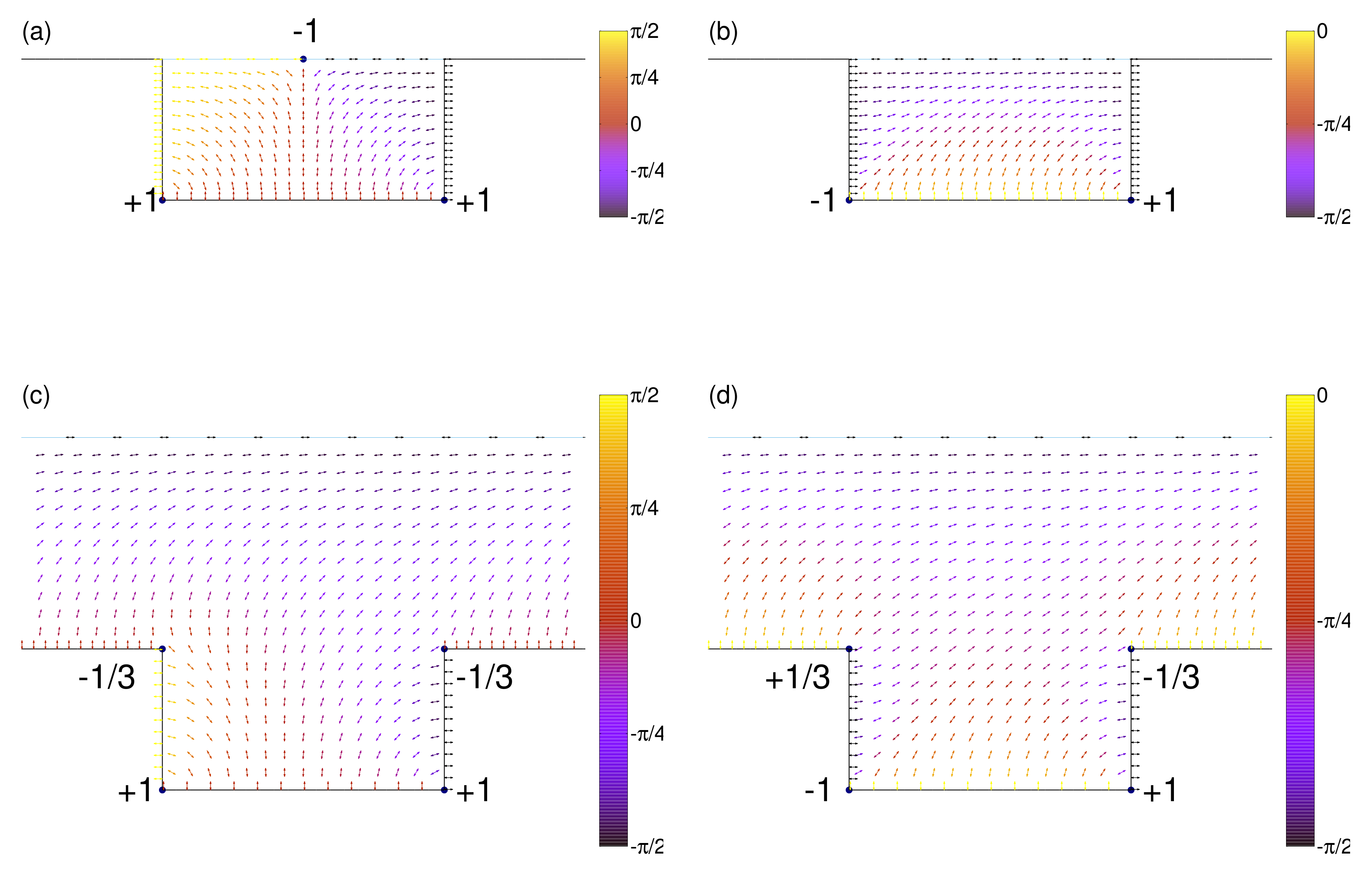
Figure 2.
Typical filled and wet textures at a crenellated substrate (, ): (a) the symmetric filled state texture; (b) the asymmetric filled state texture; (c) the symmetric wet state texture; and (d) the asymmetric wet state texture. The blue line corresponds to the position of the nematic isotropic interface, and the director field is colored by the angle of the local nematic director with respect to the y axis. Circles locate the director field singularities or disclinations and are labeled by their topological charges.

Figure 3.
Elastic contribution to the free energy of one substrate period as a function of d for the states () and the states () and substrate relief and . Three different substrate periods are shown: , 100 and 1000. For the states, the numerical results are compared to the analytical results given by Equation (A8).

Figure 4.
Interfacial phase diagram of a nematogen at the nematic–isotropic coexistence in contact with a crenellated substrate of period and (black continuous lines), (red dashed lines) and (green dot-dashed lines). The black dotted lines correspond to the phase boundaries in the limit .
Figure 4.
Interfacial phase diagram of a nematogen at the nematic–isotropic coexistence in contact with a crenellated substrate of period and (black continuous lines), (red dashed lines) and (green dot-dashed lines). The black dotted lines correspond to the phase boundaries in the limit .

Figure 5.
The same as Figure 4 for .
Figure 5.
The same as Figure 4 for .

Figure 6.
The same as Figure 4 for .
Figure 6.
The same as Figure 4 for .

Figure 7.
The same as Figure 4 for . Colored labels and identify the regions where these phases are stable for each : black for , green for and red for .
Figure 7.
The same as Figure 4 for . Colored labels and identify the regions where these phases are stable for each : black for , green for and red for .

© 2019 by the authors. Licensee MDPI, Basel, Switzerland. This article is an open access article distributed under the terms and conditions of the Creative Commons Attribution (CC BY) license (http://creativecommons.org/licenses/by/4.0/).
Share and Cite
MDPI and ACS Style
Rojas-Gómez, Ó.A.; Telo da Gama, M.M.; Romero-Enrique, J.M. Wetting of Nematic Liquid Crystals on Crenellated Substrates: A Frank–Oseen Approach. Crystals 2019, 9, 430. https://0-doi-org.brum.beds.ac.uk/10.3390/cryst9080430
AMA Style
Rojas-Gómez ÓA, Telo da Gama MM, Romero-Enrique JM. Wetting of Nematic Liquid Crystals on Crenellated Substrates: A Frank–Oseen Approach. Crystals. 2019; 9(8):430. https://0-doi-org.brum.beds.ac.uk/10.3390/cryst9080430
Chicago/Turabian StyleRojas-Gómez, Óscar A., Margarida M. Telo da Gama, and José M. Romero-Enrique. 2019. "Wetting of Nematic Liquid Crystals on Crenellated Substrates: A Frank–Oseen Approach" Crystals 9, no. 8: 430. https://0-doi-org.brum.beds.ac.uk/10.3390/cryst9080430
Note that from the first issue of 2016, this journal uses article numbers instead of page numbers. See further details here.