Feasibility of Predicting Static Dielectric Constants of Polymer Materials: A Density Functional Theory Method

 ,
,
Abstract
:
1. Introduction
2. Computational Methods
3. Results and Discussion
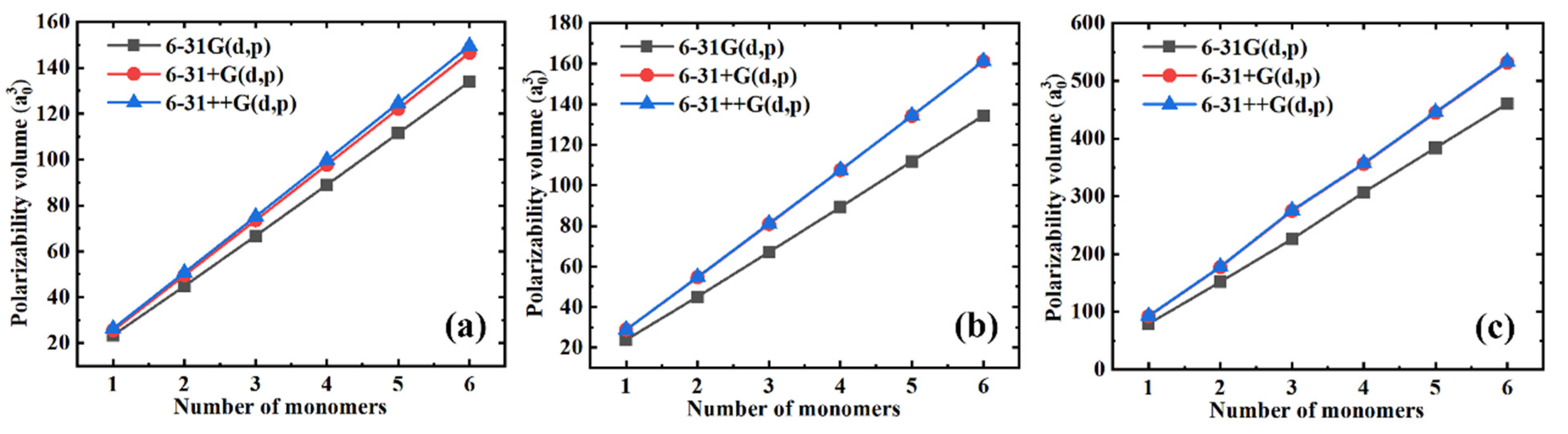
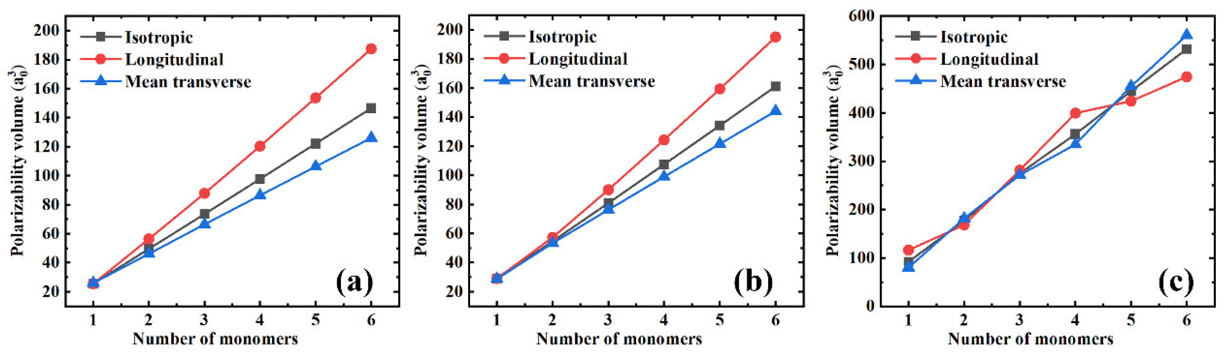
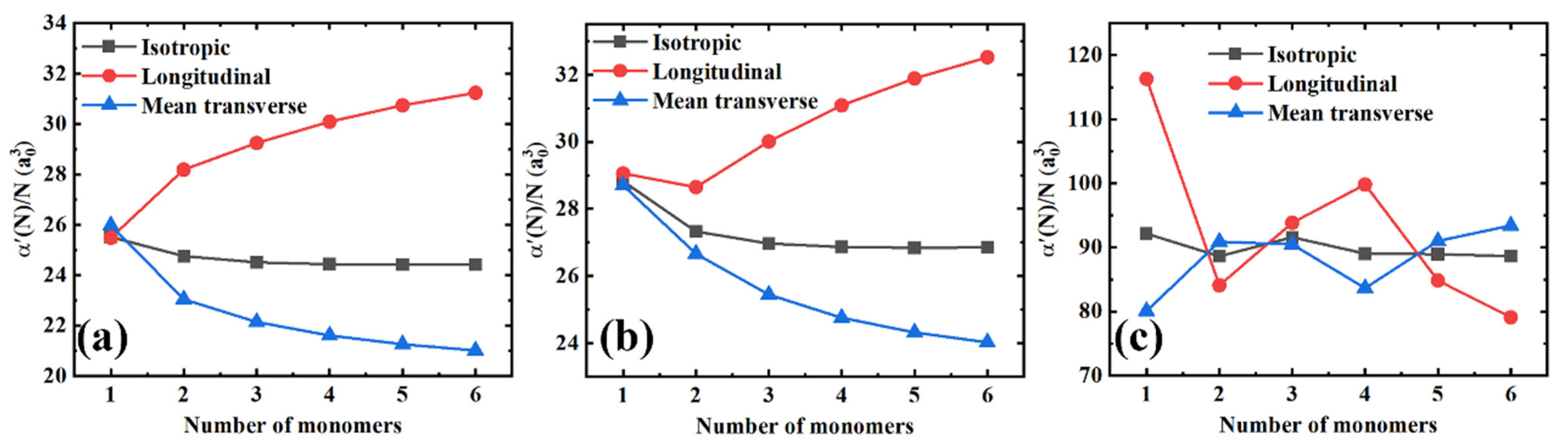
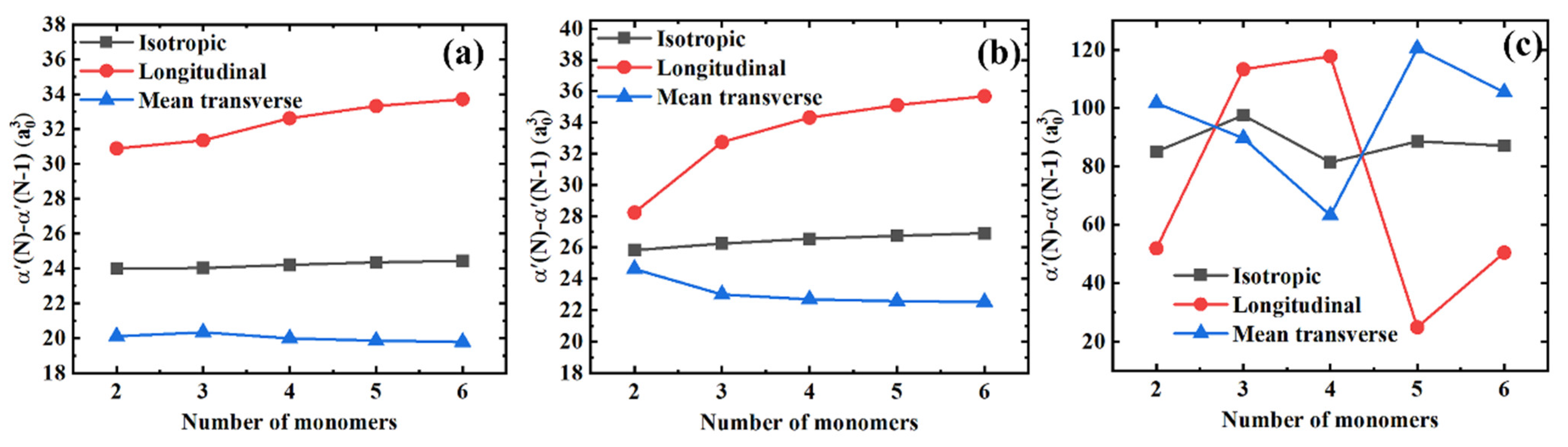
3.1. Polarizability
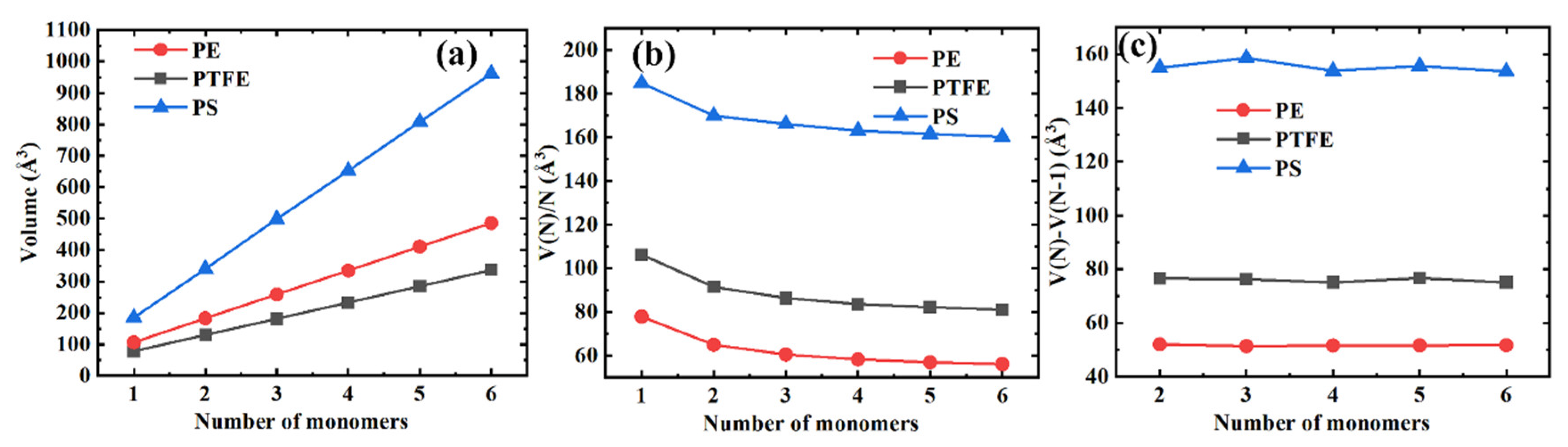
3.2. Volume
3.3. Dielectric Constant
3.4. Double Layers of Polymer Chains
4. Conclusions
Supplementary Materials
Author Contributions
Funding
Institutional Review Board Statement
Informed Consent Statement
Data Availability Statement
Conflicts of Interest
References
- Blythe, A.R.; Blythe, T.; Bloor, D. Electrical Properties of Polymers; Cambridge University Press: New York, NY, USA, 2005. [Google Scholar]
- Ahmad, Z. Polymer Dielectric Materials. In Dielectric Material; Silaghi, M.A., Ed.; IntechOpen: London, UK, 2012. [Google Scholar]
- Prathab, B.; Aminabhavi, T.M. Atomistic Simulations to Compute Surface Properties of Poly(N-vinyl-2-pyrrolidone) (PVP) and Blends of PVP/Chitosan. Langmuir 2007, 23, 5439–5444. [Google Scholar] [CrossRef] [PubMed]
- Kyrychenko, A.; Korsun, O.M.; Gubin, I.I.; Kovalenko, S.M.; Kalugin, O.N. Atomistic Simulations of Coating of Silver Nanoparticles with Poly(vinylpyrrolidone) Oligomers: Effect of Oligomer Chain Length. J. Phys. Chem. C 2015, 119, 7888–7899. [Google Scholar] [CrossRef]
- Ruuska, H.; Arola, E.; Kannus, K.; Rantala, T.T.; Valkealahti, S. Feasibility of density functional methods to predict dielectric properties of polymers. J. Chem. Phys. 2008, 128, 064109. [Google Scholar] [CrossRef] [PubMed]
- Perdew, J.P.; Wang, Y. Accurate and simple analytic representation of the electron-gas correlation energy. Phys. Rev. B 1992, 45, 13244–13249. [Google Scholar] [CrossRef] [PubMed]
- McDowell, S.A.C.; Amos, R.D.; Handy, N.C. Molecular polarisabilities—A comparison of density functional theory with standard ab initio methods. Chem. Phys. Lett. 1995, 235, 1–4. [Google Scholar] [CrossRef]
- Champagne, B.t.; Perpète, E.A.; Gisbergen, S.J.A.v.; Baerends, E.-J.; Snijders, J.G.; Soubra-Ghaoui, C.; Robins, K.A.; Kirtman, B. Assessment of conventional density functional schemes for computing the polarizabilities and hyperpolarizabilities of conjugated oligomers: An ab initio investigation of polyacetylene chains. J. Chem. Phys. 1998, 109, 10489–10498. [Google Scholar] [CrossRef] [Green Version]
- Mori-Sánchez, P.; Wu, Q.; Yang, W. Accurate polymer polarizabilities with exact exchange density-functional theory. J. Chem. Phys. 2003, 119, 11001–11004. [Google Scholar] [CrossRef]
- Lee, C.; Yang, W.; Parr, R.G. Development of the Colle-Salvetti correlation-energy formula into a functional of the electron density. Phys. Rev. B 1988, 37, 785–789. [Google Scholar] [CrossRef] [PubMed] [Green Version]
- Becke, A.D. Density-functional thermochemistry. III. The role of exact exchange. J. Chem. Phys. 1993, 98, 5648–5652. [Google Scholar] [CrossRef] [Green Version]
- Becke, A.D. A new mixing of Hartree–Fock and local density-functional theories. J. Chem. Phys. 1993, 98, 1372–1377. [Google Scholar] [CrossRef]
- Barone, V.; Adamo, C.; Lelj, F. Conformational behavior of gaseous glycine by a density functional approach. J. Chem. Phys. 1995, 102, 364–370. [Google Scholar] [CrossRef]
- Atkins, P.W.; Friedman, R.S. Molecular Quantum Mechanics; Oxford University Press: New York, NY, USA, 1997. [Google Scholar]
- Frisch, M.J.; Trucks, G.W.; Schlegel, H.B.; Scuseria, G.E.; Robb, M.A.; Cheeseman, J.R.; Scalmani, G.; Barone, V.; Petersson, G.A.; Nakatsuji, H.; et al. Gaussian 16 Rev. B.01; Gaussian, Inc.: Wallingford, CT, USA, 2016. [Google Scholar]
- Foresman, J.; Frisch, A. Exploring Chemistry with Electronic Structure Methods, 2nd ed.; Gaussian, Inc.: Pittsburgh, PA, USA, 1996. [Google Scholar]
- Rice, J.E.; Handy, N.C. The calculation of frequency-dependent polarizabilities as pseudo-energy derivatives. J. Chem. Phys. 1991, 94, 4959–4971. [Google Scholar] [CrossRef]
- Tomasi, J.; Mennucci, B.; Cammi, R. Quantum Mechanical Continuum Solvation Models. Chem. Rev. 2005, 105, 2999–3094. [Google Scholar] [CrossRef] [PubMed]
- Lee, B.; Richards, F.M. The interpretation of protein structures: Estimation of static accessibility. J. Mol. Biol. 1971, 55, 379-IN4. [Google Scholar] [CrossRef]
- Shrake, A.; Rupley, J.A. Environment and exposure to solvent of protein atoms. Lysozyme and insulin. J. Mol. Biol. 1973, 79, 351–371. [Google Scholar] [CrossRef]
- Watson, M.A.; Sałek, P.; Macak, P.; Helgaker, T. Linear-scaling formation of Kohn-Sham Hamiltonian: Application to the calculation of excitation energies and polarizabilities of large molecular systems. J. Chem. Phys. 2004, 121, 2915–2931. [Google Scholar] [CrossRef] [PubMed]
- Available online: http://www.matweb.com/search/datasheet.aspx?MatGUID=a882a1c603374e278d062f106dfda95b&ckck=1 (accessed on 1 January 2021).
- Svorčík, V.; Ekrt, O.; Rybka, V.; Lipták, J.; Hnatowicz, V. Permittivity of polyethylene and polyethyleneterephtalate. J. Mater. Sci. Lett. 2000, 19, 1843–1845. [Google Scholar] [CrossRef]
- Koizumi, N.; Yano, S.; Tsuji, F. Dielectric properties of polytetrafluoroethylene and tetrafluoroethylene-hexafluoropropylene copolymer. J. Polym. Sci. Part C Polym. Symp. 1968, 23, 499–508. [Google Scholar] [CrossRef]
- Available online: http://www.matweb.com/search/DataSheet.aspx?MatGUID=4e0b2e88eeba4aaeb18e8820f1444cdb (accessed on 1 January 2021).
- Clarricoats, P.J.B. A new waveguide method for measuring the permittivity of dielectric slabs. Proc. IEE-Part C Monogr. 1962, 109, 401–405. [Google Scholar] [CrossRef]
- Available online: http://www.matweb.com/search/DataSheet.aspx?MatGUID=1c41e50c2e324e00b0c4e419ca780304 (accessed on 1 January 2021).
- Martínez, L.; Andrade, R.; Birgin, E.G.; Martínez, J.M. PACKMOL: A package for building initial configurations for molecular dynamics simulations. J. Comput. Chem. 2009, 30, 2157–2164. [Google Scholar] [CrossRef] [PubMed]


| Name | Number of Monomers | 6-31G(d, p) | 6-31+G(d, p) | 6-31++G(d, p) |
|---|---|---|---|---|
| PE | 1 | 77.769 | 77.815 | 77.815 |
| 2 | 129.719 | 129.833 | 129.833 | |
| 3 | 181.026 | 181.191 | 181.191 | |
| 4 | 232.604 | 232.793 | 232.793 | |
| 5 | 284.233 | 284.463 | 284.463 | |
| 6 | 335.866 | 336.146 | 336.146 | |
| PTFE | 1 | 105.953 | 106.26 | 106.262 |
| 2 | 181.521 | 182.819 | 183.571 | |
| 3 | 257.166 | 259.082 | 258.579 | |
| 4 | 331.783 | 334.154 | 334.155 | |
| 5 | 407.344 | 410.814 | 410.658 | |
| 6 | 482.5 | 485.854 | 485.947 | |
| PS | 1 | 184.79 | 184.79 | 184.965 |
| 2 | 339.582 | 339.582 | 339.973 | |
| 3 | 495.189 | 495.189 | 498.268 | |
| 4 | 650.496 | 650.496 | 652.596 | |
| 5 | 805.949 | 805.949 | 808.011 | |
| 6 | 960.777 | 960.777 | 961.946 |
| Name | Molecule | Polarizability | Volume | Dielectric Constant | Experimental Value |
|---|---|---|---|---|---|
| PE | C2H6 | 25.51 | 77.815 | 1.93 | 2.2–2.3 [22,23] |
| C4H10 | 49.51 | 129.833 | 2.04 | ||
| C6H14 | 73.53 | 181.191 | 2.10 | ||
| C8H18 | 97.73 | 232.793 | 2.13 | ||
| C10H22 | 122.08 | 284.463 | 2.15 | ||
| C12H26 | 146.51 | 336.146 | 2.16 | ||
| PTFE | C2H2F4 | 28.82 | 106.26 | 1.69 | 2.0 [24,25] |
| C4H2F8 | 54.65 | 182.819 | 1.74 | ||
| C6H2F12 | 80.9 | 259.082 | 1.76 | ||
| C8H2F16 | 107.46 | 334.154 | 1.78 | ||
| C10H2F20 | 134.21 | 410.814 | 1.79 | ||
| C12H2F24 | 161.12 | 485.854 | 1.80 | ||
| PS | C8H10 | 92.78 | 184.965 | 2.48 | 2.4–2.6 [26,27] |
| C16H18 | 177.91 | 339.973 | 2.51 | ||
| C24H26 | 275.64 | 498.268 | 2.62 | ||
| C32H34 | 356.99 | 652.596 | 2.58 | ||
| C40H42 | 445.78 | 808.011 | 2.59 | ||
| C48H50 | 533.14 | 961.946 | 2.60 |
| Name | Interlayer Distances | Polarizability | Volume | Dielectric Constant | Experimental Value |
|---|---|---|---|---|---|
| PE | single layer | 146.51 | 336.146 | 2.16 | 2.2–2.3 [22,23] |
| 2.0 | 293.54 | 661.721 | 2.16 | ||
| 2.5 | 293.68 | 672.55 | 2.14 | ||
| PTFE | single layer | 161.12 | 485.854 | 1.80 | 2.0 [24,25] |
| 2.0 | 321.93 | 969.114 | 1.79 | ||
| 2.5 | 321.93 | 969.12 | 1.79 |
Publisher’s Note: MDPI stays neutral with regard to jurisdictional claims in published maps and institutional affiliations. |
© 2021 by the authors. Licensee MDPI, Basel, Switzerland. This article is an open access article distributed under the terms and conditions of the Creative Commons Attribution (CC BY) license (http://creativecommons.org/licenses/by/4.0/).
Share and Cite
Tang, Z.; Chang, C.; Bao, F.; Tian, L.; Liu, H.; Wang, M.; Zhu, C.; Xu, J. Feasibility of Predicting Static Dielectric Constants of Polymer Materials: A Density Functional Theory Method. Polymers 2021, 13, 284. https://0-doi-org.brum.beds.ac.uk/10.3390/polym13020284
Tang Z, Chang C, Bao F, Tian L, Liu H, Wang M, Zhu C, Xu J. Feasibility of Predicting Static Dielectric Constants of Polymer Materials: A Density Functional Theory Method. Polymers. 2021; 13(2):284. https://0-doi-org.brum.beds.ac.uk/10.3390/polym13020284
Chicago/Turabian StyleTang, Zheng, Chaofan Chang, Feng Bao, Lei Tian, Huichao Liu, Mingliang Wang, Caizhen Zhu, and Jian Xu. 2021. "Feasibility of Predicting Static Dielectric Constants of Polymer Materials: A Density Functional Theory Method" Polymers 13, no. 2: 284. https://0-doi-org.brum.beds.ac.uk/10.3390/polym13020284