Cohesive Fracture Study of a Bonded Coarse Silica Sand Aggregate Bond Interface Subjected to Mixed-Mode Bending Conditions

Abstract

One of the primary objectives in the design of composite structures is the prevention of premature bond failure. Therefore, the characterization of cohesive behavior is an important field of study in structural engineering. Using fracture mechanics principles, the cohesive behavior of an epoxy bonded coarse silica sand aggregate bond interface is studied in this paper, with a focus on finding a general analytical form of idealizing its behavior when used in a specimen possessing asymmetric and inhomogeneous qualities. Two series of small-scale specimens were experimentally tested under mixed-mode bending (MMB) conditions, where it was found that there was negligible influence exerted on the fracture energy of the interface due to changes in the mixed-mode ratio or initial crack length. Using finite element analysis (FEA) methods, an appropriate bilinear traction-separation model was developed to both validate as well as obtain a set of consistent parameters applicable to all tested specimens. Comparison of the Global Method and the Local Method, used to obtain partitioned Mode I and Mode II fracture energy values from MMB specimens, were made, with the conclusion that both methods are adequate in the calculation of the total fracture energy though the Local Method should be used to obtain accurate partitioned Mode I and Mode II fracture energy values. Idealization of the bond interface using the cohesive parameters derived can be accurately achieved by the use of both contact interactions and cohesive elements in two-dimensional and three-dimensional FE models, though the results obtained using contact interactions would be expected to exhibit greater global stiffness.

1. Introduction

In the study of composite structures, the behavior of the bond layer between adjacent material interfaces is of particular interest, since an effective bond is critical to achieve optimum performance of the structure rather than the undesirable premature failure at the bond interface. Fracture mechanics theories have been applied to the study of bond interface behavior, initially through the strength-based failure criterion, developed by Inglis [1], which allows for crack propagation to occur once a critical stress is reached at the interface. Subsequently, the more widely adopted Griffith approach [2] was developed, which allows for crack growth to proceed once the energy release rate attains a critical value, determined by material properties as well as the geometry of the specimen for plane stress conditions. The basis of cohesive zone models (CZM) [3] incorporate both the strength-based and energy-based criterions to analytically predict the fracture behavior at interfaces and can be used effectively to directly represent the physical bond at an interface between two adherends [4].

Abundant research has been conducted in previous decades in the effort to characterize bond behavior through a combination of experimental testing and applied analytical techniques, used in conjunction with finite element analysis (FEA) methods. Analysis of pure Mode I action (normal separation at the interface) and pure Mode II action (shear separation along the interface) have primarily been performed on homogenous specimens [5,6,7]. The introduction of factors such as mixed-mode configurations, material inhomogeneity and dimensional asymmetry into the analysis has led to the requirement of more complex analytical techniques and derivations in order to fully portray the bond behavior in a general context that would be applicable to all structural configurations [8]. By validating analytical models with experimental data, the models can then be used with confidence to predict the performance of other similar specimens, through the application of FEA methods.

The aim of this research is to determine, with reasonable accuracy, the cohesive parameters of a bonded coarse silica sand aggregate layer intended for enhanced bonding between pultruded glass fiber reinforce polymer (GFRP) plates and ultra-high performance concrete (UHPC) in full-scale hybrid beams and bridge systems [9]. This specific type of bond interface has been proven, through prior experimentation, to provide improved connection between adherends due to the combined effects of adhesive bonding and mechanical interlock. The ability to idealize the behavior of this bond interface in commercial FE software packages, such as ABAQUS, as cohesive elements through a set of consistent cohesive parameters will aid in the design and optimization of future structural members utilizing this particular bonding technique. It is critical to obtain a closed-form set of values that would be applicable to a wide spectrum of possible configurations relating to the initial crack length and applied mixed-mode ratios. The desired outcome is a general set of consistent cohesive element parameters that can be used in future two-dimensional (2D) and three-dimensional (3D) FE models.

This paper includes three main portions. The first section covers an extensive experimental study of small-scale specimens tested under mixed-mode bending (MMB) loading conditions with attention towards the relationship between the applied mode-mixity as well as the crack length initially introduced in the specimen with respect to the bond performance. In the subsequent section, two distinct numerical methods, the Global [7] and Local Methods [8], will be introduced with the goal of deriving partitioned Mode I and Mode II formulas for the determination of key cohesive parameters from experimental data. The last portion of the paper will bring together all of the previous findings in this study, in which the results from a multi-stage FE parametric study performed in both 2D and 3D environments will be discussed.

2. Research Significance

The research performed in this study broadens the current understanding regarding the state-of-the-art of bond interface behavior through detailed experimental and numerical analysis of an epoxy bonded coarse silica sand aggregate layer, an improved method of bonding between high performance materials. The findings provide a closed-form method for the derivation of consistent partitioned cohesive parameters for MMB specimens. The set of parameters, validated for both 2D and 3D modeling environments in ABAQUS, include considerations for factors such as material inhomogeneity and geometric asymmetry.

3. Experimental Testing of Mixed-Mode Bending Specimens

3.1. Introduction

For the determination of the cohesive bond properties, MMB specimens were chosen. The advantage of testing a single series of MMB specimens compared with parallel tests of double cantilever beams (DCB) and end-notch flexure (ENF) specimens is the intermixed nature of the Mode I and Mode II behaviors, allowing for interactions between the cohesive laws governing each failure mode [10]. It also allows for the simultaneous establishment of Mode I and Mode II parameters, though at the expense of more complex analytical calculations.

3.2. Design and Construction of Specimens

The tested specimens consisted of a 9.6 mm thick pultruded GFRP plate bonded to a 50 mm thick cast-in-place layer of UHPC via the epoxy bonded coarse silica sand aggregate layer, with a constant length and width of 460 and 130 mm, respectively, for the entire specimen. The MMB specimens were designed based on the concepts presented in ASTM Standard D6671-06 [11], with modifications made due to the asymmetric and dissimilar bilayer nature of the test cross-section. The cross-section dimensions were also partly determined from previous experimentation [9] on full-scale beam specimens, where it was necessary to maintain an identical height ratio between the GFRP and the UHPC layers in order to allow for ease of comparison between the small-scale and full-scale tests. The intended bonding surface of the GFRP plate was first coarsened using a belt sander and a coarsening stone to improve bonding. Coarse silica sand aggregates, with diameters ranging from 4.5 to 9.0 mm, were then bonded to the surface using a 1 mm thick layer of Sikadur^® 32 epoxy [12]. The desired initial crack length was obtained by providing bonded coarse silica sand aggregate layer up to a defined boundary on the GFRP plate as well as placing a thin barrier between the GFRP and UHPC during curing in order to prevent contact. Allowing for an epoxy curing timeframe of 7 days, the UHPC was cast directly overtop of the bonded coarse silica sand aggregate layer. At the ends of the specimen, aluminum angles (L76 × 76 × 5) were bonded to the GFRP plate, which will be fully attached to the steel apparatus during testing.

3.3. Material Properties

The GFRP plates used were specified by the manufacturer to have a minimum flexural strength of 400 MPa with a flexural modulus of elasticity equal to or greater than 25 GPa [13]. Similarly, manufacturer specifications for the UHPC provide an ultimate compressive strength within the range of 150–180 MPa at 28 days, with an associated modulus of elasticity between 50 and 60 GPa [14]. The epoxy adhesive used for bonding of the coarse silica sand aggregate layer is a moisture insensitive epoxy adhesive; according to manufacturer specifications, the epoxy has a tensile strength of 30 MPa and a modulus of elasticity equal to 3.8 GPa [12].

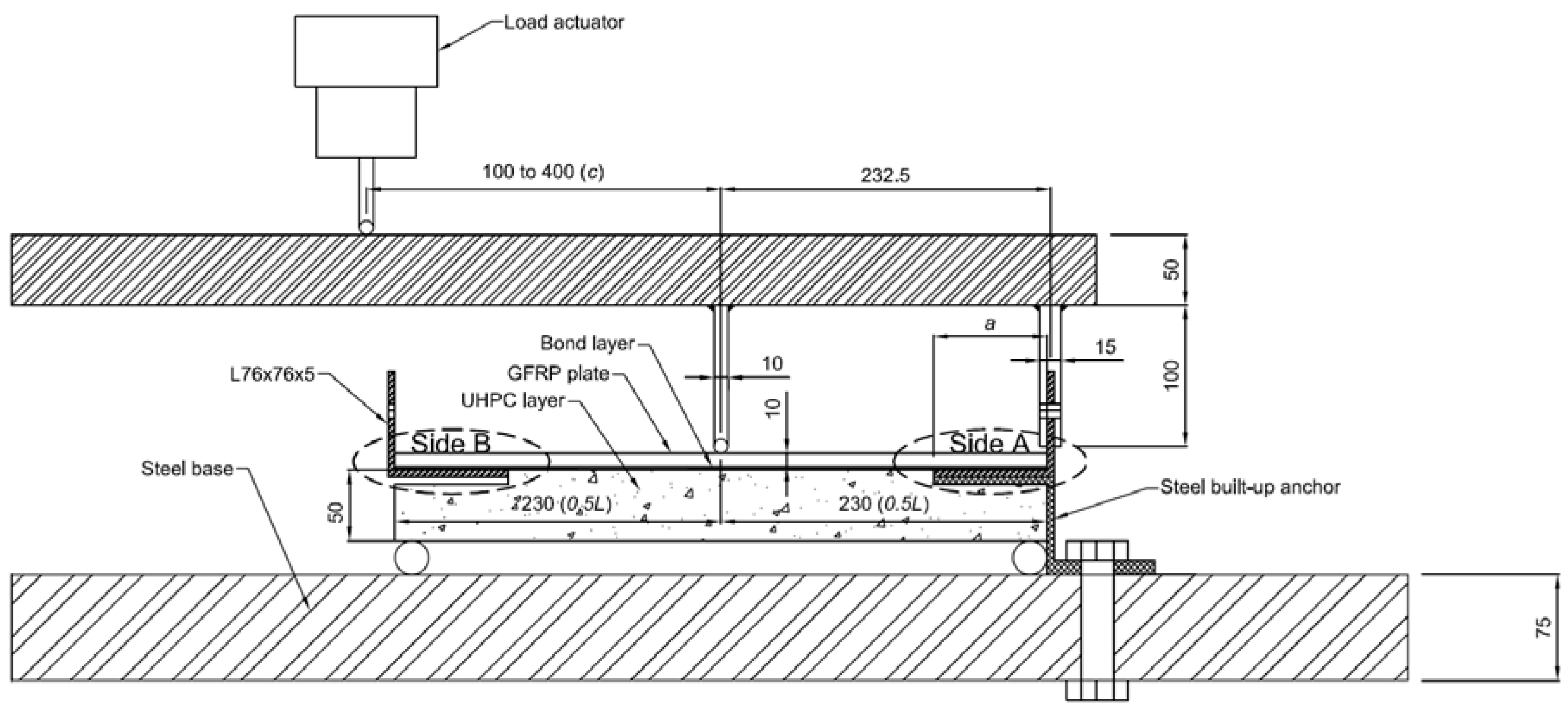
3.4. Testing Set-Up and Instrumentation

Experimental testing of MMB specimens using a test matrix of varying initial crack lengths and mixed-mode ratios was conducted. In order to optimize the number of possible test specimens, the test configuration and dimensions allowed for the cohesive interfaces from both ends of the specimen to be tested. The test matrix, with the specimen IDs, is presented in Table 1.

Table 1. Test matrix and specimen IDs.

Specimen ID	Initial crack length (a) (mm)	Moment arm (c) (mm)
S-a80-c250	80	250
S-a100-c250	100	250
S-a120-c100	120	100
S-a120-c175	120	175
S-a120-c250	120	250
S-a120-c325	120	325
S-a120-c400	120	400
S-a140-c250	140	250
S-a160-c250	160	250

Table 1. Test matrix and specimen IDs.

Specimen ID	Initial crack length (a) (mm)	Moment arm (c) (mm)
S-a80-c250	80	250
S-a100-c250	100	250
S-a120-c100	120	100
S-a120-c175	120	175
S-a120-c250	120	250
S-a120-c325	120	325
S-a120-c400	120	400
S-a140-c250	140	250
S-a160-c250	160	250

The values for the crack lengths and moment arms were chosen to maximize the diversity of configurations tested, with crack lengths ranging incrementally from 0 to 0.5 L and the moment arms varying between 0 and L, where L is the full length of the specimen. The applied mode-mixity to the specimen can be easily adjusted by altering the length of the applied moment arm, which should not be influenced by the initial crack length of the specimen [15]. The full test set-up, with dimensions in mm, is shown in Figure 1.

Testing was conducted under displacement control mode, with a vertical loading rate of 1 mm/min at the load actuator. Three linear variable differential transformers (LVDTs) were positioned at quarter-positions along the top of the GFRP plate. Since both sides of all specimens were to be tested, the first tested side (Side A) was loaded up to and past the peak load, in a manner that would provide an adequate depiction of its behavior. It was then unloaded prior to the onset of unstable crack propagation along the bond interface, once the crack growth approached the mid-span of the specimen. The second tested side (Side B) was, however, allowed to undergo complete failure.

Figure 1. Specimen dimensions and test set-up (all dimensions are in mm).

Figure 1. Specimen dimensions and test set-up (all dimensions are in mm).

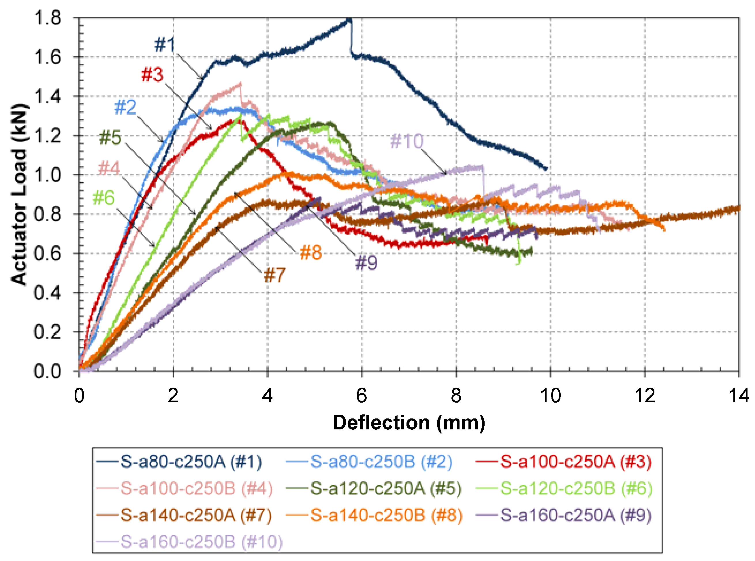
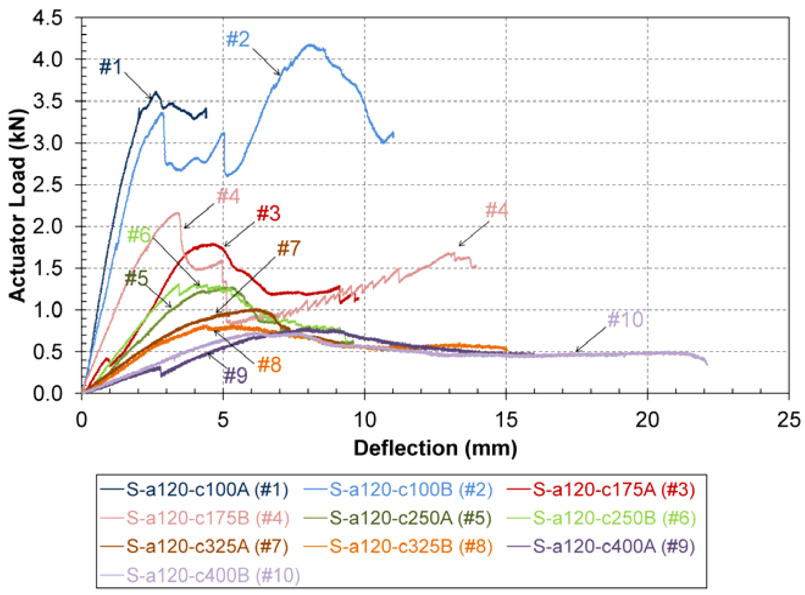
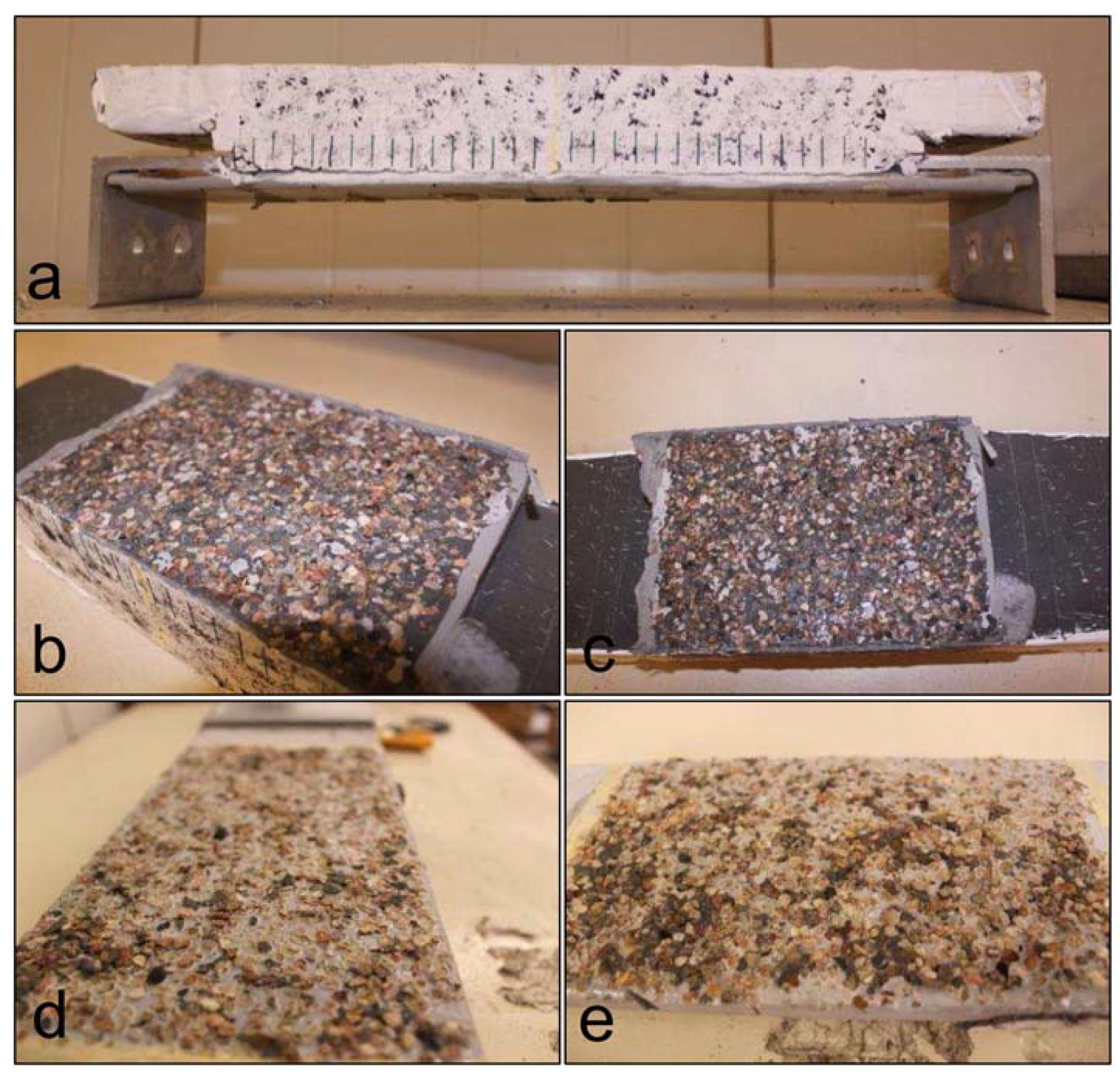
3.5. Experimental Results

The load-deflection curves, describing the relationship between the applied actuator load and the downward displacement at the point of load application, from the nine tested specimens (with two sets of data obtained for each specimen) are presented in Figure 2 and Figure 3. In order to allow for suitable comparisons, the specimens tested using a moment arm (c) equal to 250 mm are provided in Figure 2, where the specimens tested with a crack length (a) equal to 120 mm are compared with one another in Figure 3.

Figure 2. Experimental load-deflection comparison for specimens tested at c = 250 mm.

Figure 2. Experimental load-deflection comparison for specimens tested at c = 250 mm.

Figure 3. Experimental load-deflection comparison for specimens tested at a = 120 mm.

Figure 3. Experimental load-deflection comparison for specimens tested at a = 120 mm.

Complete debonding, characterized by separation of the GFRP plate from the UHPC layer, occurred in all of the tested specimens except for S-a120-c100, S-a120-c250 and S-a80-c250; in these specimens, tensile cracking in the UHPC layer within the flexural region was observed without separation of the GFRP plate from the UHPC layer. Tensile cracking in the UHPC may have been due to higher stress field concentrations caused by a reduction in the UHPC thickness at the ends of the specimens; the additional space was used to accommodate the steel built-up anchor, as shown previously in Figure 1. Representative photographs showing the condition of the specimens after failure are provided in Figure 4.

All of the tested specimens exhibited near linear-elastic behavior during the first phase of loading up to the peak load. Once the load applied approached the peak load, the global stiffness of all the specimens was observed to decrease, where some of the load-deflection curves peaked at the maximum load and others demonstrated a smooth transition through a zero slope plateau. Past the peak load, crack propagation commenced and it was seen that the specimens did continue to provide resistance to the applied load, though typically at a level lower than the peak load. The decrease in strength was particular dramatic for specimens with crack lengths (a) below 140 mm as well as at applied moment arm lengths (c) less than 325 mm, where the final residual strength approached 50% of the peak load. For specimens with crack lengths (a) equal to and greater than 140 mm or with an applied moment arm length (c) equal to or greater than 325 mm, the residual strength provided appeared to reach an asymptotic value representing more than 60% of its peak strength. The one exception to these trends was seen in Specimen S-a120-c100B where the strength of the bond interface was actually seen to increase after reaching the damage initiation point. This result does require further attention but can be assumed as an irregularity in the overall observed behavior of this bond interface. As a whole, it can be generally stated that the bond interface behaves nearly linear-elastically up to a geometrically influenced maximum load, after which a declining level of residual strength is expected along the interface during crack propagation until ultimate failure occurs.

Figure 4. Representative photographs illustrating typical failure mode: (a) Elevation view of specimen after failure; (b) Longitudinal view of bond interface on the Ultra-High Performance Concrete (UHPC) layer; (c) Top view of bond interface on UHPC layer; (d) Longitudinal view of bond interface on Glass Fiber Reinforce Polymer (GFRP) plate and (e) Top view of bond interface on GFRP plate.

Figure 4. Representative photographs illustrating typical failure mode: (a) Elevation view of specimen after failure; (b) Longitudinal view of bond interface on the Ultra-High Performance Concrete (UHPC) layer; (c) Top view of bond interface on UHPC layer; (d) Longitudinal view of bond interface on Glass Fiber Reinforce Polymer (GFRP) plate and (e) Top view of bond interface on GFRP plate.

4. Numerical Analysis for Cohesive Parameters

4.1. Introduction

Typically, in bond behavior studies where at least one of the adherends is a cementitious material such as reinforced concrete, two types of cohesive failure mechanism are considered. The first is failure through the interior of the adhesive layer and the second is interface cracking within the concrete adherend. However, the unique combination of high performance materials used in this study, namely GFRP and UHPC, allows for the elimination of the latter failure mechanism. This is due to the enhanced overall strength of the UHPC confirmed through previous studies [14] so that the tensile cracking strength of the UHPC greatly exceeds that of the cohesive layer.

The typical cohesive parameters used to characterize the behavior of a bond interface in the CZM are: the critical fracture energy, effective nominal stress, the damage initiation ratio and the initial material stiffness per unit area. For simple test configurations in elastic homogeneous specimens, the cohesive parameters can be easily derived from calculations based on the experimental load-deflection curve. Nevertheless, with increasing complexities, such as the introduction of mixed-mode loading, asymmetry in the cross-sectional dimensions as well as an inhomogeneous composition, more detailed derivations will be required to determine the cohesive parameters. Various research studies have been conducted over the years with the objective of obtaining accurate methods to numerically determine values for fracture energy under different configurations. These studies include considerations for loading configurations [16], mixed-mode partitioning [17,18,19], interface rigidity [20] as well as other factors. Two different methods, the Global Method and the Local Method, will be discussed and compared in this section.

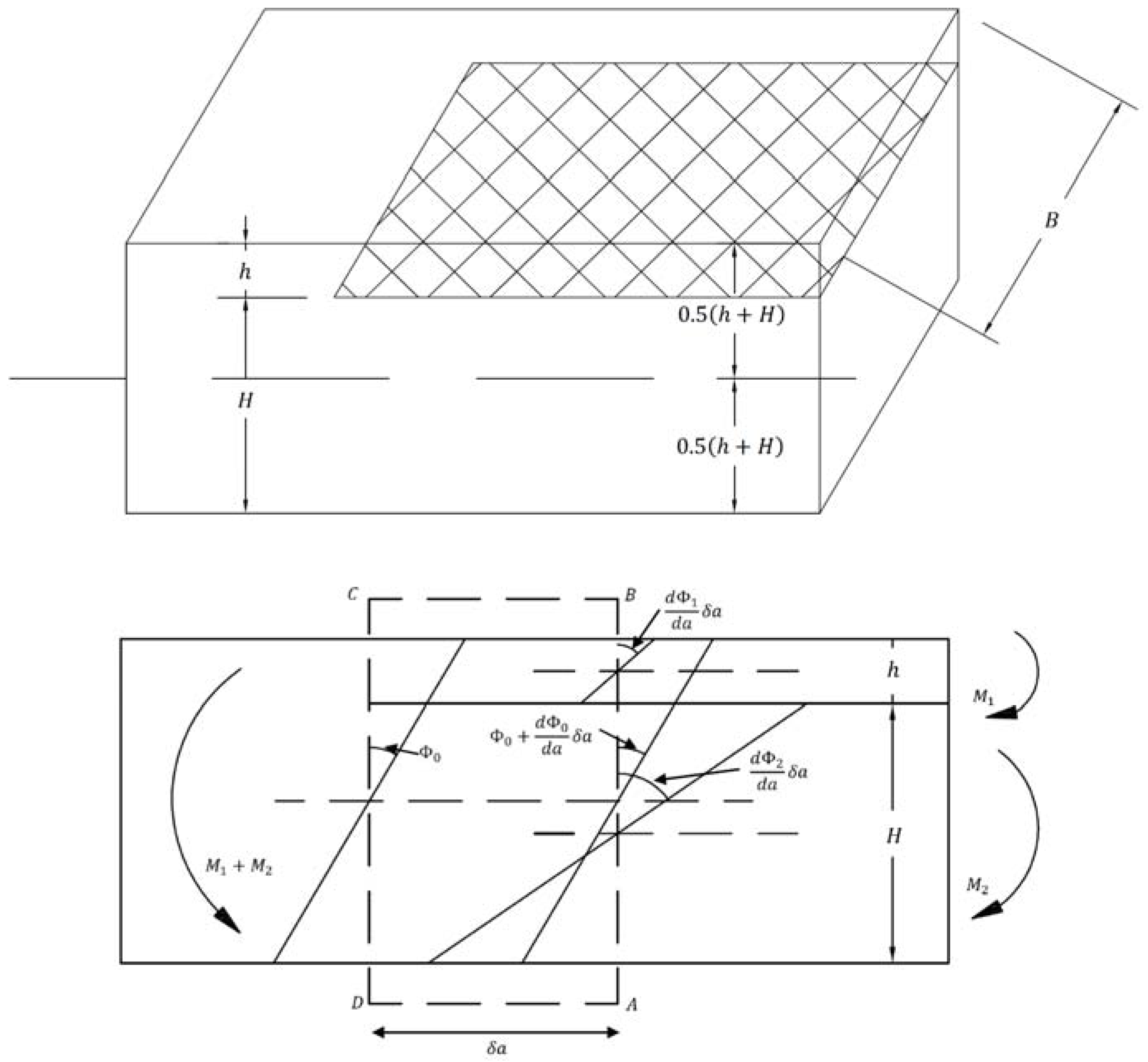
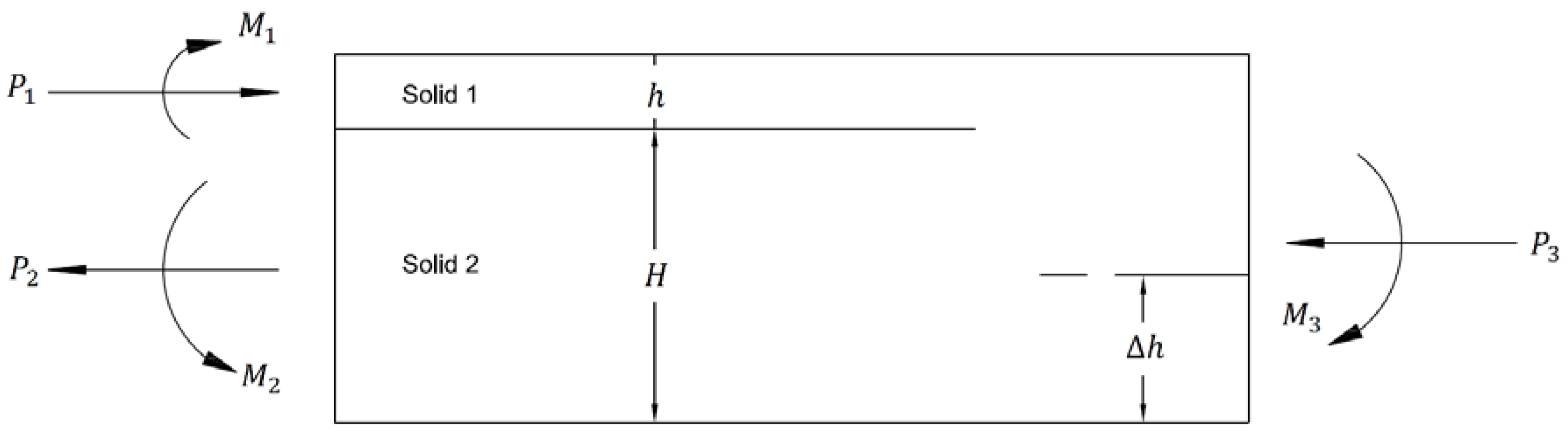
4.2. Derived Relationships for Fracture Energy

4.2.1. Global Method

Williams [7] developed the Global Method, an analytical technique for calculating the total fracture energy of an asymmetric bilayer composed of dissimilar materials based on beam theory and crack tip contour rotations; however, the relationships for how to partition the total fracture energy into its Mode I and Mode II components were derived only for a homogenous cross-section made up of one material. For the purpose of this research, the existing formulation of the Global Method was expanded to include the influence of asymmetry and inhomogeneous specimens in the partitioned fracture energy values.

In this following section, an extension to the work originally completed by Williams, derived by the authors, will be presented, resulting in a set of equations for the partitioned critical fracture energy for a MMB asymmetric bilayer specimen with an inhomogeneous cross-section. A diagram illustrating the components of the crack tip contour rotation is provided in Figure 5.

Figure 5. Diagram illustrating crack tip contour rotations used in the Global Method [7].

Figure 5. Diagram illustrating crack tip contour rotations used in the Global Method [7].

Given a height factor, ξ, equal to:

(1)

It follows that the expression for the moment of inertia are:

(2)

I₁ = 8I₀ξ³

(3)

I₂ = 8I₀(1 − ξ)³

(4)

Expanding on the equations derived by Williams [7],

(5)

(6)

where U_e and U_s are the external work performed and the strain energy, respectively, and EI_eq is the equivalent flexural stiffness of the uncracked portion.

The total fracture energy, G, is given as follows:

(7)

In order to obtain the fracture energy associated specifically with Mode I and II action, the applied moments can be described by the following linear combinations:

M₁ = M_I + M_II

(8)

M₂ = λM_I + ψM_II

(9)

To determine the value of the coefficients λ and ψ, the following two statements are made:

1.

Under pure Mode II loading,

(10a)

(10b)

(10c)

(10d)

2.

Under pure Mode I loading,

M₁ = M₂

(11a)

M_I + M_II = λM _I + ψM_II

(11b)

λ = −1

(11c)

Substituting the expressions for M₁ and M₂ obtained from Equations (8) to (11) into the expression for the total fracture energy [Equation (7)] and partitioning based on the components relating to M_I and M_II, we can obtain the equations for the partitioned fracture energy shown below in Equations (12) and (13).

(12)

(13)

where:

(14)

(15)

The total fracture energy would be equal to the linear sum between Equations (12) and (13), with the following relationship, where:

G_T = G_I + G_II

(16)

The equivalent flexural stiffness, EI_eq, can be calculated by transforming the composite section into an equivalent section composed of solely Material 1 in both the upper and lower arm, with an equivalent neutral axis, y, where:

(17)

(18)

4.2.2. Local Method

Hutchinson and Suo [8] conducted a similar research to Williams [7] to identify the partitioned fracture energy of a MMB asymmetric bilayer (meaning two layers of dissimilar materials in the cross-section) specimen. The theory used for the derivation of the Local Method focused on the crack tip stress field in the area of the crack propagation in order to obtain values for the partitioned stress intensity factors (K_I and K_II), which are then used to calculate the partitioned fracture energy values. A summary of the derivation and the resulting relationship is provided in this section. For reference to the some of the components described in the derivation, a diagram is provided in Figure 6.

Figure 6. Diagram illustrating crack tip stress field parameters used in the Local Method.

Figure 6. Diagram illustrating crack tip stress field parameters used in the Local Method.

Dundurs’ elastic mismatch parameters, where α measures the mismatch in the in-plane tensile modulus across the interface and β measures the mismatch in the in-plane bulk modulus, are given as:

(19)

(20)

where:

(21)

(22)

The complex interface equivalent modulus of elasticity is given as:

(23)

The neutral axis of the composite beam ahead of the crack can be found at a distance of Δh where:

(24)

(25)

(26)

with h equal to the depth of the upper layer and H equal to the depth of the bottom layer.

The dimensionless cross-section, A, and moment of inertia, I, are:

(27)

(28)

with the following geometric factors:

(29a)

(29b)

(29c)

(30)

(31)

(32)

ω = 52.1° − 3° η

(33)

The complex stress intensity factor, K, is as follows:

(34)

(35)

where:

(36)

M = M₁ − C₃M₃

(37)

The complex stress intensity factor can be partitioned into its Mode I (real) and Mode II (imaginary) components, where K_I and K_II, respectively, are as follows:

(38)

(39)

The total energy release rate for crack advance in the interface, G_T, can also be linearly partitioned into its Mode I and Mode II components, using the following relationship:

(40a)

where:

(40b)

(40c)

4.3. Considerations for Correction Factors and Non-Linearity Effects

Firstly, it should be noted that the effect of the apparatus weight was not considered in the derivations presented in Section 4.2. As stated in ASTM Standard D6671-06, lever weight correction factors may need to be included when the weight of the apparatus is greater than 3% of the maximum applied load [11]. Nevertheless, a preliminary investigation was conducted to examine the changes in the derived fracture energy values when the lever weight correction factor is included and results showed that there was minimal (less than 1%) increase in the derived fracture energy values. This phenomenon was also observed in similar experimental studies conducted by other researchers [21].

Possible nonlinearity on the experimental results produced by the configuration of the loading apparatus used, specifically in regards to the horizontal force induced in the system at higher actuator displacements, should also be considered. It was found through previous research that the application of load above the lever arm may induce nonlinearity in the results, sometimes up to 30% [22], which can be detected through increased specimen stiffness at higher displacements. This effect, however, was not exhibited in all of the tested specimens, as shown in Figure 2 and Figure 3. Nevertheless, an in-depth investigation should also be performed to determine the influence of the moment exerted on the specimen due to the horizontal force induced on the lever arm. The angle of rotation for the lever arm was first calculated at peak load condition after which the horizontal force along the length of the lever arm was calculated as a percentage of the vertically applied actuator load. Finally, the moment exerted on the specimen by the horizontal force was determined, using a moment arm equal to 150 mm, which is the height above the specimen where the actuator load is applied. The nonlinearity effect was then calculated as a percentage of the imposed moment from the vertical load. A summary of the steps described above is tabulated in Table 2.

The investigation conducted above shows that the nonlinearity effect due to the horizontal force induced in the lever arm is within a range between 1% and 4%. The difference is thereby demonstrated to be marginal and in line with the expected error for MMB testing [22]. Therefore, the application of the derived fracture energy relationships in Section 4.2 to the experimental data can provide sound results and will be used for further analysis shown in subsequent sections in this paper.

Table 2. Nonlinearity imposed due to induced horizontal force on lever arm.

Specimen ID	Angle of rotation (degrees)	Horizontal Force (kN)	Moment (kNm)		Nonlinearity due to horizontal force (%)
			Horizontal Force	Vertical Force
S-a80-c250A	0.66	0.018	0.003	0.394	1
S-a80-c250B	0.64	0.015	0.002	0.336	1
S-a100-c250A	0.77	0.017	0.003	0.317	1
S-a100-c250B	0.65	0.016	0.002	0.351	1
S-a120-c100A	1.56	0.097	0.015	0.362	4
S-a120-c100B	1.69	0.10	0.015	0.336	4
S-a120-c175A	1.50	0.047	0.007	0.314	2
S-a120-c175B	1.10	0.042	0.006	0.379	2
S-a120-c250A	0.93	0.020	0.003	0.301	1
S-a120-c250B	0.78	0.018	0.003	0.325	1
S-a120-c325A	1.0	0.017	0.003	0.315	1
S-a120-c325B	0.76	0.011	0.002	0.261	1
S-a120-c400A	1.03	0.014	0.002	0.300	1
S-a120-c400B	1.09	0.014	0.002	0.291	1
S-a140-c250A	0.93	0.014	0.002	0.218	1
S-a140-c250B	0.97	0.017	0.003	0.250	1
S-a160-c250A	1.17	0.018	0.003	0.222	1
S-a160-c250B	1.54	0.026	0.004	0.240	2

Table 2. Nonlinearity imposed due to induced horizontal force on lever arm.

Specimen ID	Angle of rotation (degrees)	Horizontal Force (kN)	Moment (kNm)		Nonlinearity due to horizontal force (%)
			Horizontal Force	Vertical Force
S-a80-c250A	0.66	0.018	0.003	0.394	1
S-a80-c250B	0.64	0.015	0.002	0.336	1
S-a100-c250A	0.77	0.017	0.003	0.317	1
S-a100-c250B	0.65	0.016	0.002	0.351	1
S-a120-c100A	1.56	0.097	0.015	0.362	4
S-a120-c100B	1.69	0.10	0.015	0.336	4
S-a120-c175A	1.50	0.047	0.007	0.314	2
S-a120-c175B	1.10	0.042	0.006	0.379	2
S-a120-c250A	0.93	0.020	0.003	0.301	1
S-a120-c250B	0.78	0.018	0.003	0.325	1
S-a120-c325A	1.0	0.017	0.003	0.315	1
S-a120-c325B	0.76	0.011	0.002	0.261	1
S-a120-c400A	1.03	0.014	0.002	0.300	1
S-a120-c400B	1.09	0.014	0.002	0.291	1
S-a140-c250A	0.93	0.014	0.002	0.218	1
S-a140-c250B	0.97	0.017	0.003	0.250	1
S-a160-c250A	1.17	0.018	0.003	0.222	1
S-a160-c250B	1.54	0.026	0.004	0.240	2

4.4. Application of Derived Relationships to Experimental Data

The two analytical techniques, in the form presented in the Section 4.2 [with Equations (12), (13) and (16) along with Equation (40a–c) used for the Global and Local Method, respectively], were applied to the experimental data obtained from the nine MMB specimens (Section 3), where the value for the fracture energy was obtained at the maximum load condition. For comparison, the total fracture energy (G_T) as well as the partitioned Mode I and Mode II fracture energy values (G_I and G_II) obtained from the two techniques were examined. In the case of the Local Method, the two sets of results obtained using either plane stress or plane strain assumptions were calculated. A summary of the comparison is shown in Table 3.

Firstly, a comparison between the values of total fracture energy obtained through the two different techniques showed that identical results (or near identical results in the case of the plane strain formulation using the Local Method) were obtained, which agrees with similar previous studies [18]. This authenticates the overarching concepts used in the development of both methodologies prior to partitioning. Taking a more in-depth investigation into the partitioned fracture energy values, it is evident that the Global Method dedicates the bulk of the total fracture energy to Mode I contributions, while the Local Method allows for a more even distribution of Mode I and Mode II contributions. From the literature, it has been extensively discussed for homogeneous specimens that the participation of Mode I is severely exaggerated using the Global Method due to overly rigid fixity assumptions in the cross-section at the location of the crack front [5,6,23,24], leading to further refinement of the original method in order to more correctly depict the support fixity. It can be confirmed from this extended investigation into asymmetric inhomogeneous specimens that the same phenomenon is present [4,8,25]. Judging from previous works [26], the expected range for the mixed-mode ratio is approximately 0 to 5, though this relationship does not take into account the influence of asymmetry or inhomogeneity in the cross-section. This range corresponds with the results obtained from both the plane strain and plane stress condition assessments using the Local Method. From the initial confirmation of the total fracture energy results with the Global Method as well as good correlation with established research results for the mixed-mode ratio, the calculated values for the partitioned fracture energy using the Local Method are considered applicable for use in this investigation and will be used as the basis of further analysis in this paper.

Table 3. Comparison of derived fracture energy.

Specimen ID	Global Method [7]				Local Method (plane stress) [8]				Local Method (plane strain) [8]
	GT	GI	GII	GI/GII	GT	GI	GII	GI/GII	GT	GI	GII	GI/GII
S-a80-c250	0.443	0.443	0.0002	2138	0.443	0.196	0.247	0.792	0.421	0.186	0.235	0.792
S-a100-c250	0.335	0.335	0.0002	2138	0.335	0.148	0.187	0.792	0.319	0.141	0.178	0.792
S-a120-c100	0.966	0.965	0.0013	721	0.966	0.412	0.554	0.743	0.919	0.392	0.527	0.743
S-a120-c175	0.769	0.769	0.0005	1470	0.769	0.336	0.433	0.777	0.732	0.320	0.412	0.777
S-a120-c250	0.662	0.662	0.0003	2138	0.662	0.292	0.370	0.792	0.370	0.278	0.352	0.792
S-a120-c325	0.572	0.572	0.0002	2704	0.572	0.254	0.318	0.799	0.544	0.242	0.302	0.799
S-a120-c400	0.597	0.596	0.0002	3179	0.597	0.266	0.331	0.804	0.568	0.252	0.315	0.804
S-a140-c250	0.491	0.491	0.0002	2138	0.491	0.217	0.274	0.792	0.467	0.206	0.261	0.792
S-a160-c250	0.668	0.668	0.0003	2138	0.668	0.295	0.373	0.792	0.636	0.281	0.355	0.792

Note: fracture energy values provided in kJ/m².

Table 3. Comparison of derived fracture energy.

Specimen ID	Global Method [7]				Local Method (plane stress) [8]				Local Method (plane strain) [8]
	GT	GI	GII	GI/GII	GT	GI	GII	GI/GII	GT	GI	GII	GI/GII
S-a80-c250	0.443	0.443	0.0002	2138	0.443	0.196	0.247	0.792	0.421	0.186	0.235	0.792
S-a100-c250	0.335	0.335	0.0002	2138	0.335	0.148	0.187	0.792	0.319	0.141	0.178	0.792
S-a120-c100	0.966	0.965	0.0013	721	0.966	0.412	0.554	0.743	0.919	0.392	0.527	0.743
S-a120-c175	0.769	0.769	0.0005	1470	0.769	0.336	0.433	0.777	0.732	0.320	0.412	0.777
S-a120-c250	0.662	0.662	0.0003	2138	0.662	0.292	0.370	0.792	0.370	0.278	0.352	0.792
S-a120-c325	0.572	0.572	0.0002	2704	0.572	0.254	0.318	0.799	0.544	0.242	0.302	0.799
S-a120-c400	0.597	0.596	0.0002	3179	0.597	0.266	0.331	0.804	0.568	0.252	0.315	0.804
S-a140-c250	0.491	0.491	0.0002	2138	0.491	0.217	0.274	0.792	0.467	0.206	0.261	0.792
S-a160-c250	0.668	0.668	0.0003	2138	0.668	0.295	0.373	0.792	0.636	0.281	0.355	0.792

Note: fracture energy values provided in kJ/m².

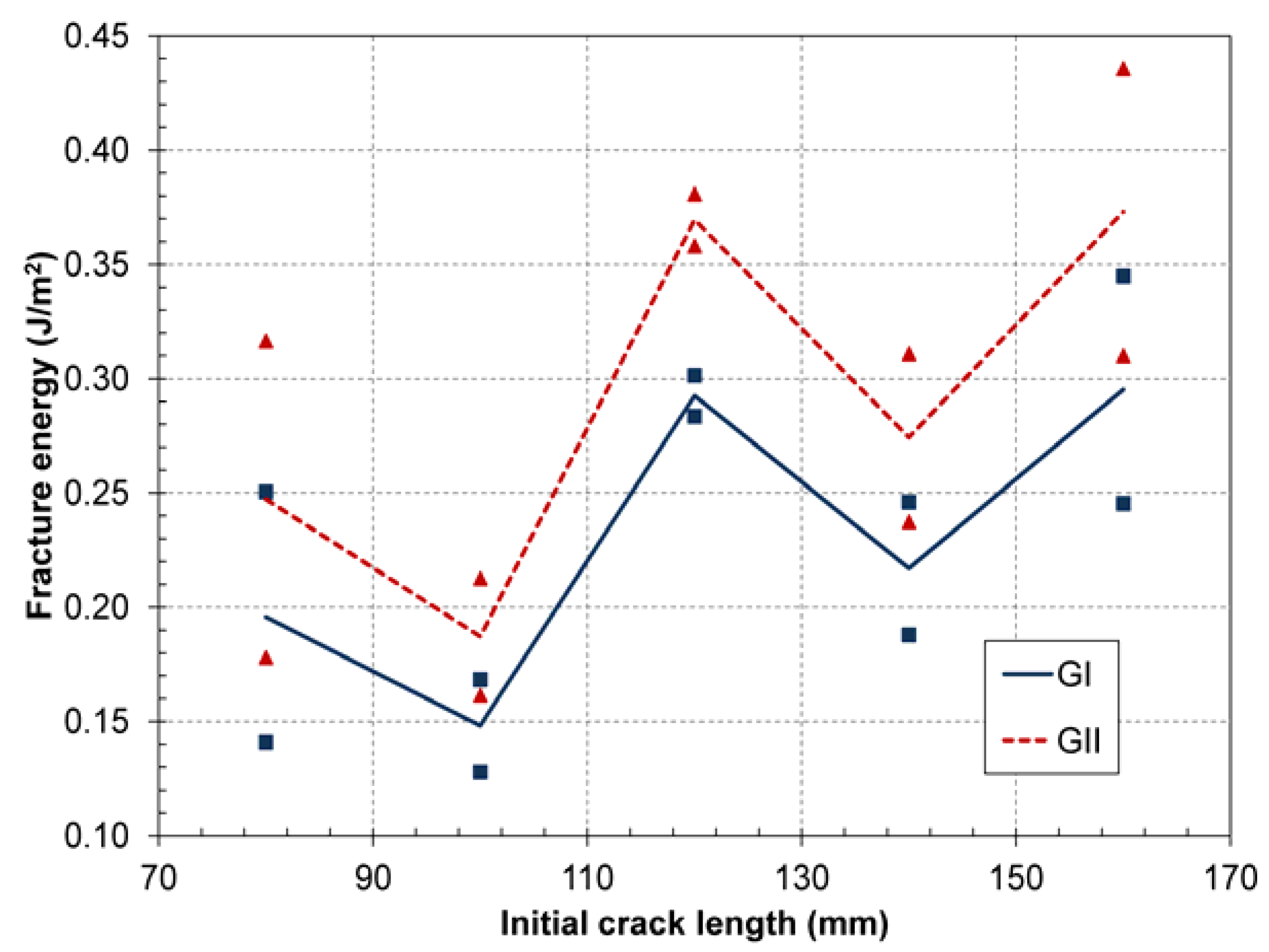
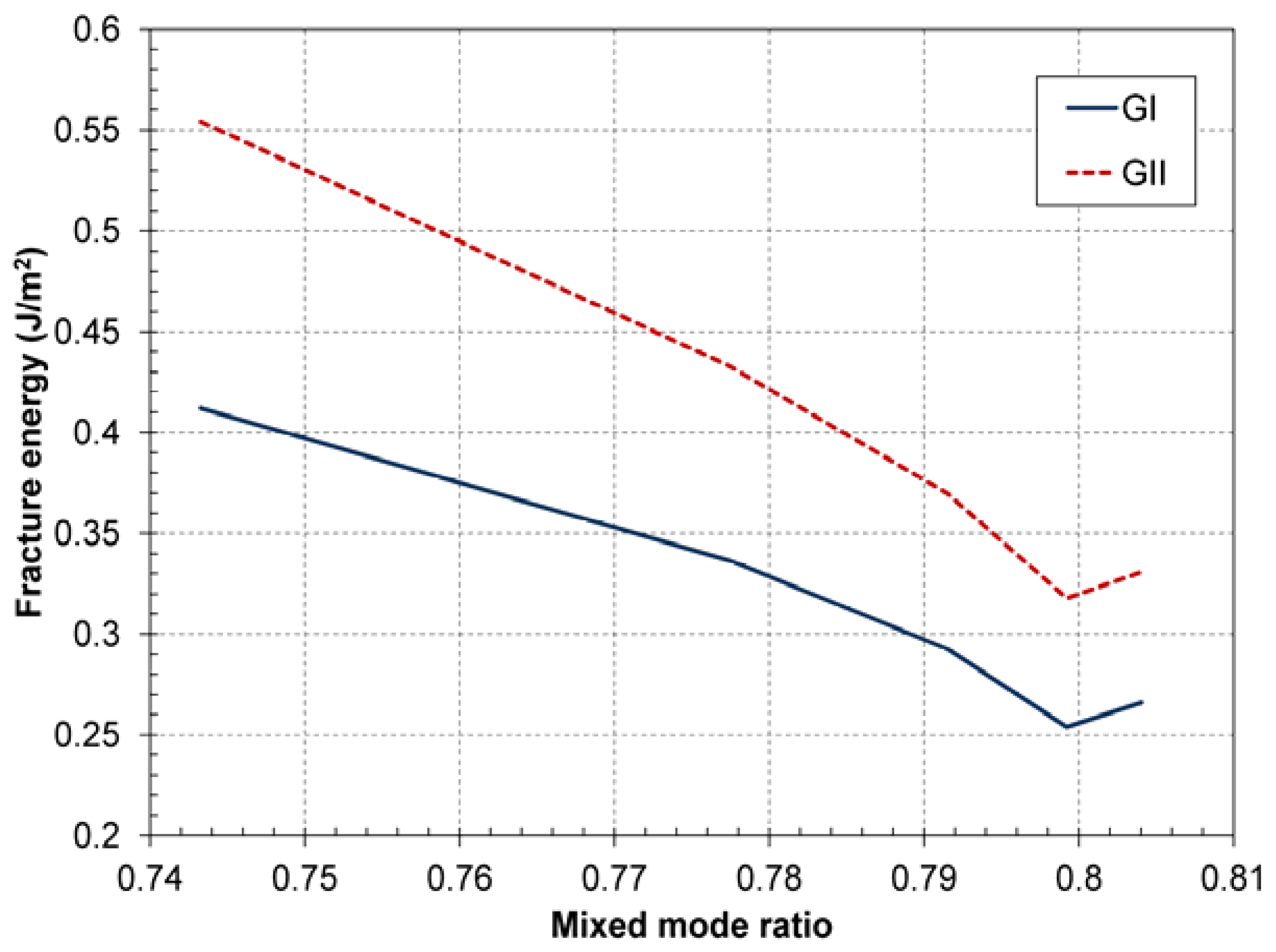
4.5. Trends of Partitioned Fracture Energy to Crack Length and Mode-Mixity

A brief discussion pertaining to the relationship between changes in test configurations and the resulting fracture parameters will be presented here. For ease of analysis, the plane stress partitioned fracture energy values calculated using the Local Method (as given in Table 3) are presented graphically in relation to the initial crack length and applied mixed-mode ratio in Figure 7 and Figure 8, respectively. For consistent comparisons, the data from all of the specimens tested using an initial crack length (a) equal to 120 mm is provided in Figure 7 and the results from the specimens tested with a moment arm (c) of 250 mm is provided in Figure 8.

In regards to the effects of changing the initial crack length of the specimen, it is difficult to determine a reliable relationship due to the large scattered nature of the data points; the small number of duplicate tests for each test configuration is also a contributing factor. The R²—value associated with an assumed linear relationship of 0.442 indicates an extremely weak correlation that can be stated as statistically irrelevant. By conducting an analysis of variance (ANOVA) single factor test based on a 95% confidence level, it was indeed found that there was no statistically significant difference between the groups tested, representing the influence of changing initial crack length on the fracture energy, where F-ratio was equal to 2.97, and less than the F_crit value of 5.19. This result indicates that the energy release rate associated with a unit area surface crack is independent of the initial length of the crack. Investigation into existing literature performed to evaluate the R-curve behavior has indicated a possible relationship between the crack length and the fracture energy required for crack propagation depending on the properties of the material tested [24,27,28,29]. Thus, deeper examination into the particular type of bond used in this research is required. To determine representative cohesive parameters applicable for use in the subsequent FE analysis, the average value of all the data collected was taken as an estimate of the Mode I and Mode II fracture energies at failure.

Figure 7. Relationship between partitioned fracture energy and initial crack length.

Figure 7. Relationship between partitioned fracture energy and initial crack length.

Figure 8. Relationship between partitioned fracture energy and applied mode-mixity ratio.

Figure 8. Relationship between partitioned fracture energy and applied mode-mixity ratio.

Similarly, when examining the correlation between the fracture energy and the applied mixed-mode ratio, it was found that as the mixed-mode ratio increased (by the application of the force through a longer moment arm and thereby increasing the relative magnitude of the Mode I mechanism with respect to the Mode II mechanism), the total fracture energy would decrease in a near linear fashion. Since it has been shown that faster loading rates during experimentation would increase the perceived fracture energy of the interface [10], this phenomenon can be attributed to the constant rate of displacement controlled loading applied at the location of the actuator, which resulted in a change of effective applied rate of displacement applied at the crack tip at various moment arms.

4.6. Applicability of Derived Partitioned Critical Fracture Energy

From the theorem of minimum energy, the equilibrium of a conservative system deformed by surface forces must be achieved in such a way that the total potential energy of the system would reach a minimum state [2]. In fracture mechanics applications, the fracture energy or energy release rate is defined as the potential energy released during the surface propagation of an increment of crack length. Thus, during crack propagation, the driving force applied must be equal to or greater than the critical fracture energy in order for stable and unstable crack propagation, respectively, to take place [30].

In order for the derived fracture energy values to be applicable for use through the traction-separation model (which will be discussed in further detail in Section 5), the critical fracture energy must be determined for each individual mode in order for the linear power law failure criterion to be properly assessed. The linear power law failure criterion describes the critical fracture energy failure envelop, discussed in detail by other researchers in related studies [16], which can be defined by the following failure criterion:

(41)

It is important to realize that the calculated values for the partitioned fracture energy (Table 3) are the maximum values reached during experimentation under a controlled mode-mixity ratio and may not reflect the pure Mode I and II critical fracture energy values associated with the cohesive layer. In all of the specimens tested, it was observed that the failure mechanism occurred primarily as a result of vertical separation at the interface due to Mode I action. Thus, it is evident that the Mode II fracture energy obtained from the experimental testing does not truly reflect the pure Mode II critical fracture energy of the interface since shear failure was not observed. Another point of view would be to recognize that the mixed-mode ratio was in fact a controlled parameter of the experimental tests, which would limit the exhibited ratio between the Mode I and Mode II fracture energy regardless of their critical values, as defined by material properties.

It can, therefore, be concluded that the critical fracture energy under pure Mode I loading can be taken as the value obtained from the experimental testing of the specimens whereas the critical fracture energy under pure Mode II loading would be a value greater than the calculated value of each individual specimens. It is for this reason that the derived expressions for fracture energy and stress intensity factors provided in Section 4.2 do not contain the subscript “c” since, depending on the loading conditions, they may not necessarily describe the critical parameters. This phenomenon will be discussed in further detail in later sections of this paper.

5. Finite Element Analysis: Validation and Consistent Parameters

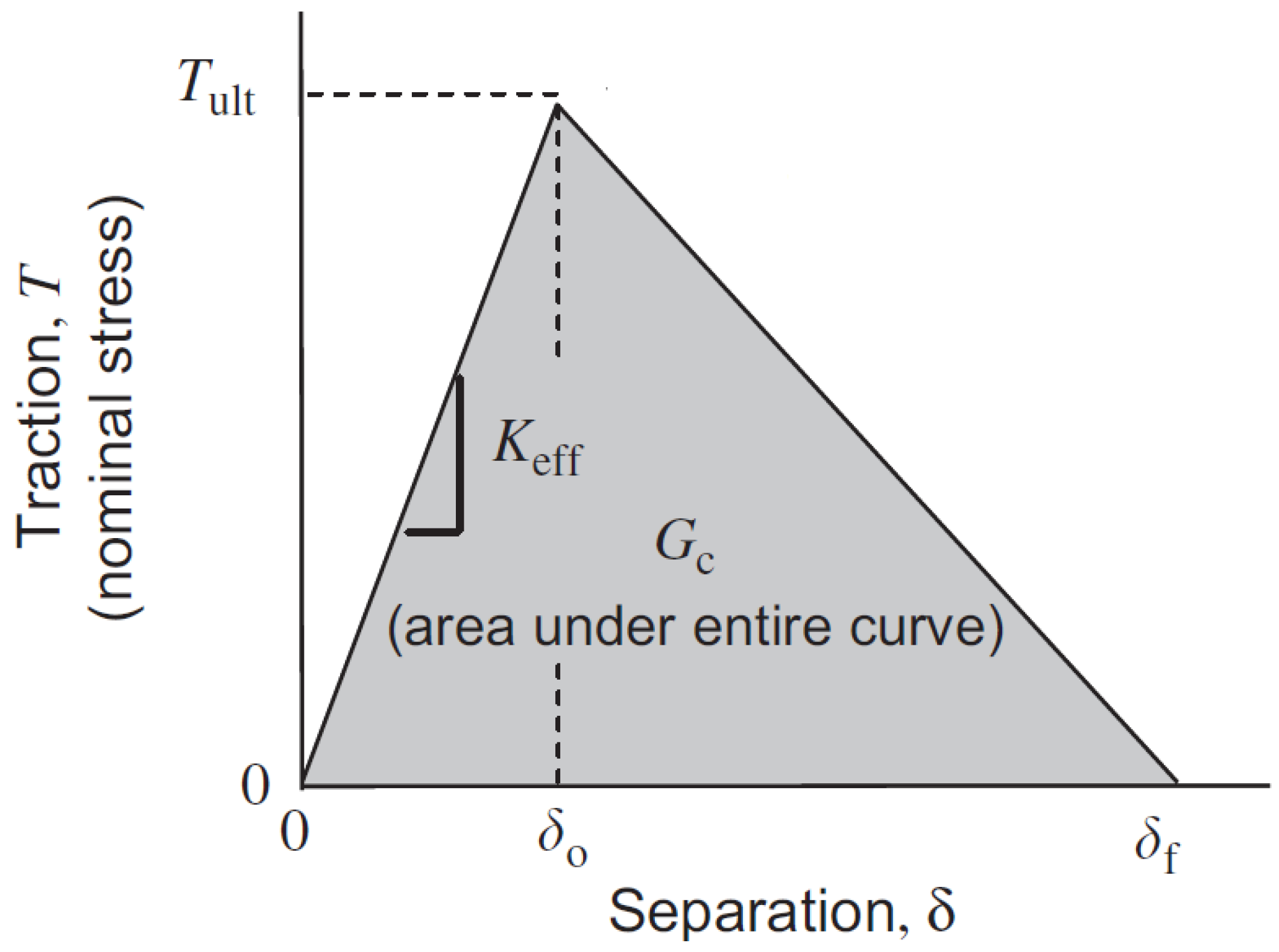
5.1. Composition of Traction-Separation Model

From the analytical derivations performed in Section 4.2, the obtained values for the partitioned Mode I and Mode II fracture energy can be used in the development of a traction-separation model for the idealization of the bond interface using cohesive elements in finite element analysis (FEA). There is an ongoing research on the degree of influence that the shape of the traction-separation model, whether triangular, trapezoidal or sinusoidal, exerts on the overall behavior of the bond interface in comparison with the influence of the critical fracture energy input and other cohesive parameters [4,31,32,33,34]. More recent research indicates the low degree of influence of the traction-separation law shape towards the modeled bond behavior, and thus, for model simplicity and compatibility with the formulation of cohesive elements in ABAQUS, a bilinear model was chosen. As mentioned previously, a typical traction-separation model is characterized by four inter-related parameters: the critical fracture energy (G_c), the effective nominal stress (T_ult), the damage initiation ratio (δ_ratio) and the initial material stiffness per unit area (K_eff). Of the four parameters, the most important parameter that would influence the behavior of the cohesive element is the critical fracture energy [35], which is equal to the total area under the bilinear traction-separation model. The bilinear model and the four parameters are shown in Figure 9.

Figure 9. Cohesive parameters of a typical bilinear traction-separation model [35].

Figure 9. Cohesive parameters of a typical bilinear traction-separation model [35].

The relationships between each of the parameters is given as:

(42)

(43)

(44)

The above four parameters are specific to the corresponding Mode I and Mode II critical fracture energy values and do not necessarily need to be the same for both failure modes.

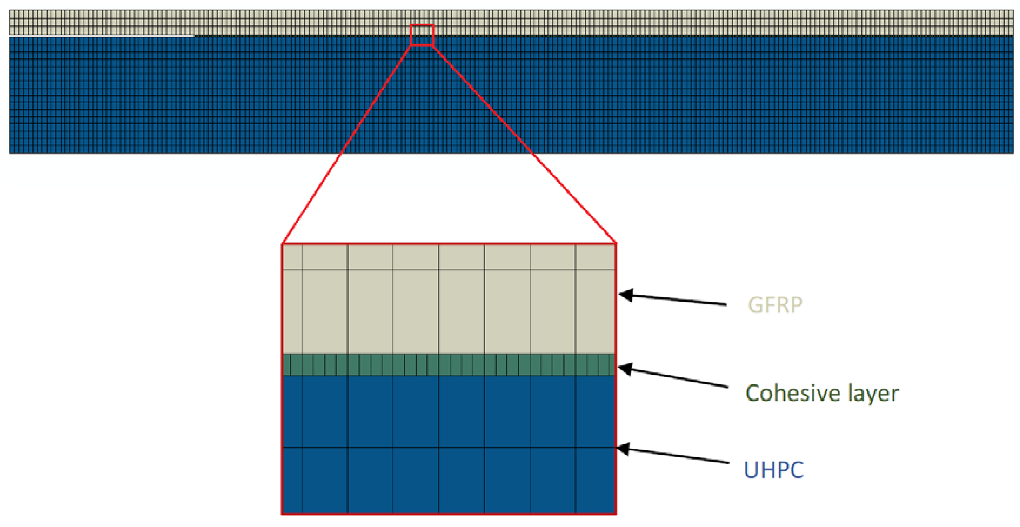
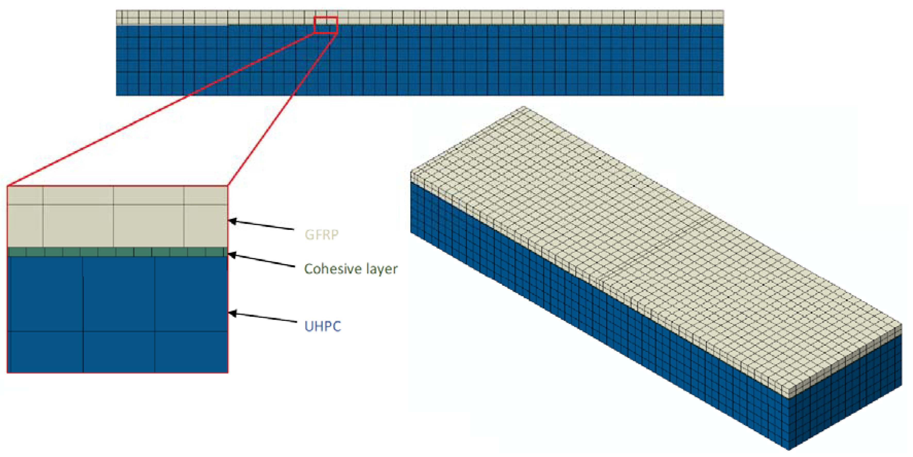
5.2. FE Model Development

The FE model was developed using ABAQUS 6.9. In the case of the 2D FE model, plane stress quadratic quadrilateral elements were used for both the GFRP and UHPC materials. Three layers of elements were used to represent the GFRP layer with a mesh size in the longitudinal direction equal to 2 mm. The same longitudinal mesh size was used for the UHPC block, with a total of 17 layers through its depth. The layer of cohesive elements, when used in the model, was tied at the top and bottom to the adjacent GFRP and UHPC material parts and had a thickness equal to 1 mm, with a longitudinal mesh size of 0.5 mm; this allowed for a 4:1 mesh ratio between the cohesive elements and the adjacent materials. Similarly, for the three-dimensional FE model, linear 3D stress brick elements used. For the GFRP material part, two layers of elements were used with an average mesh size equal to 8 mm in the longitudinal and transverse directions. The UHPC material part had a mesh size equal to approximately 8 mm in all three dimensions. Lastly, the 1 mm thick cohesive layer had a mesh size of approximately 2 mm in order to provide the same 4:1 mesh ratio that was used in the 2D FE model. Representative diagrams showing the fully developed 2D and 3D models are shown in Figure 10 and Figure 11.

The cohesive properties were modeled using the power law form of the energy criterion, with a power exponent equal to unity. The failure criterion of the cohesive interface can be expressed by the following equation [36]

(45)

where the last component of Equation (44) comprising of the Mode III fracture energy ratio is not applicable for the 2D model. This expression is the same as the mixed-mode failure criterion described in Section 4.5 [Equation (41)], with the inclusion of Mode III effects.

Figure 10. Diagram of developed 2D FE model.

Figure 10. Diagram of developed 2D FE model.

Figure 11. Diagram of developed 3D FE model.

Figure 11. Diagram of developed 3D FE model.

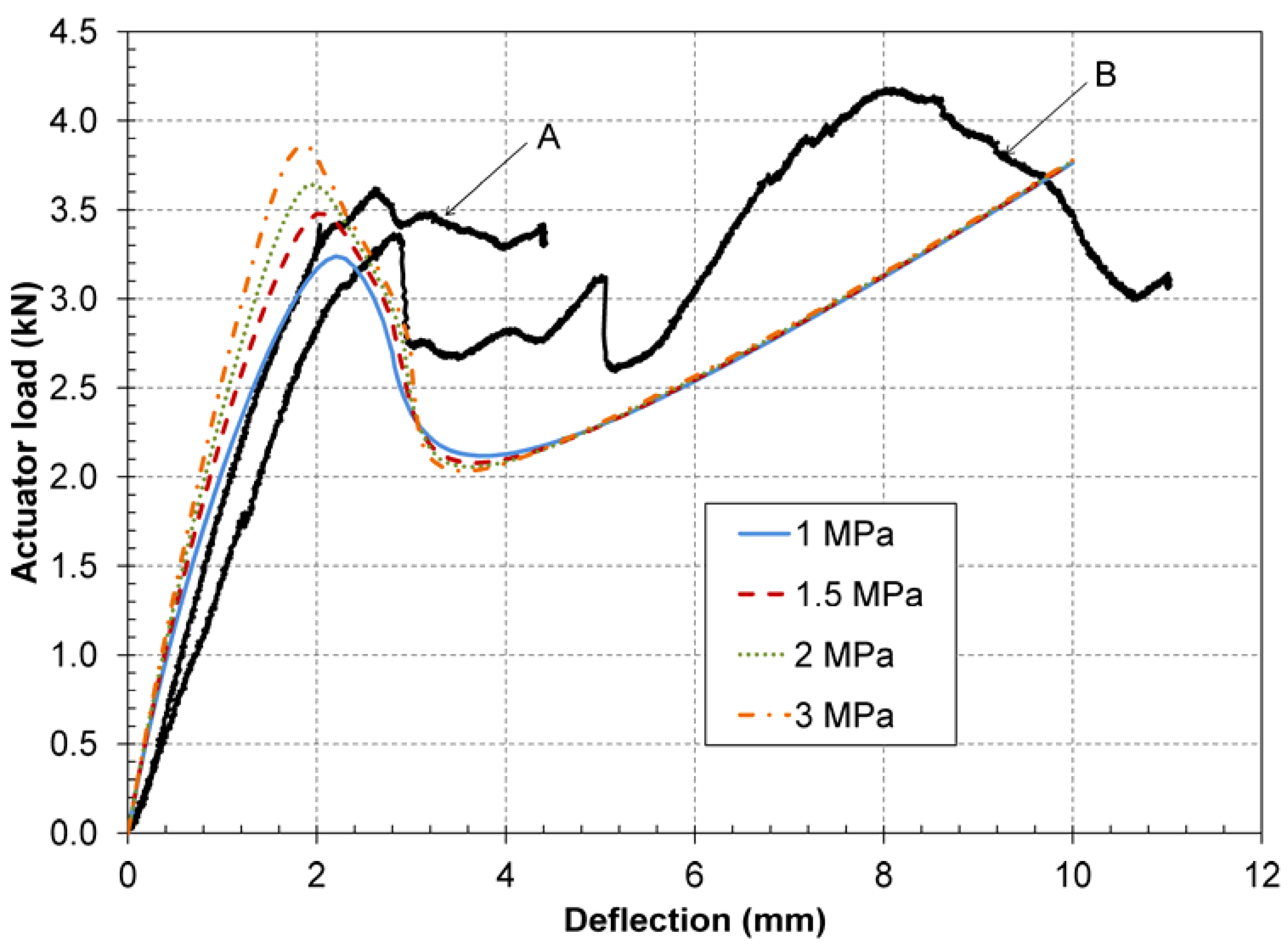
5.3. Two-Dimensional FE Model: Parametric Study and Model Validation

For the initial 2D parametric study, the bond interface was idealized using a contact interaction, with the input parameters for the traction-separation model equal to those obtained from experimental tests. The advantage of using contact interactions rather than a layer of cohesive element for modeling the bond interface is that it allows for an additional simplification of the traction-separation model as a two-parameter model for each mode by assuming a default contact penalty constraint to the interaction. This imposes cohesive constraints in the normal and shear direction without the need to provide the values for the initial material stiffness. The assumption effectively removes all influences from the shape of the traction-separation model, which eliminates the dependence on the initial material stiffness as well as the damage initiation ratio.

Using this initial simplification, a parametric study was then performed by using effective nominal stress values for Mode I equal to 1, 1.5, 2, and 3 MPa in order to determine the cohesive strength of the bond system; this method for determining the cohesive strength is in line with techniques used by other researchers [37]. The full parametric test matrix for Specimen S-a120-c100 is shown in Table 4 with the load-deflection comparison between the FEA results and experimental data, where curves A and B represent the experimental results from Sides A and B, respectively, provided in Figure 12.

Table 4. Parametric study matrix for Specimen S-a120-c100.

Model ID	Fracture energy (G) (kJ/m2)				Effective nominal stress (Tult) (MPa)
	Per unit width (mm)		Per 130 mm width		Per unit width (mm)		Per 130 mm width
	GI	GII	GI	GII	(Tult)I	(Tult)II	(Tult)I	(Tult)II
S-a120-c100-1MPa-v 2D	0.412	0.554	53.55	72.05	1.0	1.35	130	174.90
S-a120-c100-1.5MPa-v 2D	0.412	0.554	53.55	72.05	1.5	2.02	195	262.36
S-a120-c100-2MPa-v 2D	0.412	0.554	53.55	72.05	2.0	2.69	260	349.81
S-a120-c100-3MPa-v 2D	0.412	0.554	53.55	72.05	3.0	4.04	390	524.71

Table 4. Parametric study matrix for Specimen S-a120-c100.

Model ID	Fracture energy (G) (kJ/m2)				Effective nominal stress (Tult) (MPa)
	Per unit width (mm)		Per 130 mm width		Per unit width (mm)		Per 130 mm width
	GI	GII	GI	GII	(Tult)I	(Tult)II	(Tult)I	(Tult)II
S-a120-c100-1MPa-v 2D	0.412	0.554	53.55	72.05	1.0	1.35	130	174.90
S-a120-c100-1.5MPa-v 2D	0.412	0.554	53.55	72.05	1.5	2.02	195	262.36
S-a120-c100-2MPa-v 2D	0.412	0.554	53.55	72.05	2.0	2.69	260	349.81
S-a120-c100-3MPa-v 2D	0.412	0.554	53.55	72.05	3.0	4.04	390	524.71

Figure 12. Load deflection comparison for finite element analysis (FEA) of S-a120-c100 with parametric study of Mode I effective nominal stress.

Figure 12. Load deflection comparison for finite element analysis (FEA) of S-a120-c100 with parametric study of Mode I effective nominal stress.

By visual comparison, it was observed that the Model S-a120-c100-2MPa-v most closely coincided with experimental results. In order to confirm this hypothesis, the defining properties from Model S-a120-c100-2MPa-v were applied to the other eight MMB configurations tested, using the parameters given in Table 5. A comprehensive comparison between the FEA results and the experimental data show very good correlation, allowing for the model to be validated with a Mode I nominal effective stress of 2 MPa.

Table 5. Model validation parameters for mixed-mode bending (MMB) specimens.

Model ID	Fracture energy (G) (kJ/m2)				Effective nominal stress (Tult) (MPa)
	Per unit width (mm)		Per 130 mm width		Per unit width (mm)		Per 130 mm width
	GI	GII	GI	GII	(Tult)I	(Tult)II	(Tult)I	(Tult)II
S-a80-c250-2MPa-v 2D	0.196	0.247	25.44	32	2	2.53	260	328
S-a100-c250-2MPa-v 2D	0.148	0.187	19.25	24	2	2.53	260	328
S-a120-c100-2MPa-v 2D	0.412	0.554	53.55	72	2	2.69	260	350
S-a120-c175-2MPa-v 2D	0.336	0.433	43.73	56	2	2.57	260	334
S-a120-c250-2MPa-v 2D	0.292	0.370	38.02	48	2	2.53	260	328
S-a120-c325-2MPa-v 2D	0.254	0.318	33.01	41	2	2.50	260	325
S-a120-c400-2MPa-v 2D	0.266	0.331	34.56	43	2	2.49	260	323
S-a140-c250-2MPa-v 2D	0.217	0.274	28.21	36	2	2.53	260	328
S-a160-c250-2MPa-v 2D	0.295	0.373	38.38	48	2	2.53	260	328

Table 5. Model validation parameters for mixed-mode bending (MMB) specimens.

Model ID	Fracture energy (G) (kJ/m2)				Effective nominal stress (Tult) (MPa)
	Per unit width (mm)		Per 130 mm width		Per unit width (mm)		Per 130 mm width
	GI	GII	GI	GII	(Tult)I	(Tult)II	(Tult)I	(Tult)II
S-a80-c250-2MPa-v 2D	0.196	0.247	25.44	32	2	2.53	260	328
S-a100-c250-2MPa-v 2D	0.148	0.187	19.25	24	2	2.53	260	328
S-a120-c100-2MPa-v 2D	0.412	0.554	53.55	72	2	2.69	260	350
S-a120-c175-2MPa-v 2D	0.336	0.433	43.73	56	2	2.57	260	334
S-a120-c250-2MPa-v 2D	0.292	0.370	38.02	48	2	2.53	260	328
S-a120-c325-2MPa-v 2D	0.254	0.318	33.01	41	2	2.50	260	325
S-a120-c400-2MPa-v 2D	0.266	0.331	34.56	43	2	2.49	260	323
S-a140-c250-2MPa-v 2D	0.217	0.274	28.21	36	2	2.53	260	328
S-a160-c250-2MPa-v 2D	0.295	0.373	38.38	48	2	2.53	260	328

5.4. Determination of Consistent Parameters of Traction-Separation Model

For more in-depth and precise examination, the initial simplification used in the validation step (Section 5.3) to impose a default contact penalty constraint was removed. In order to minimize the number of independent variables in the traction-separation model, through examination of the relative proportion of the displacements at the onset of damage initiation and that at/near failure, it was assumed that the Mode I and Mode II damage initiation ratio was identical and equal to 5; the effect of this assumption was determined to be insignificant in relation to the influence of the fracture energy and effective nominal stress values [4,35]. Therefore, with reference to Equations (42) and (43), a change in the partitioned fracture energy would correspond to a proportional change in the value of the effective nominal stress of the affected failure mode. Based on previous experimental tests performed on the bonded coarse silica sand aggregate layer using small-scale specimens tested in a pure Mode II loading condition [38,39], a critical partitioned fracture energy ratio of 0.33 was chosen, where the critical fracture energy in Mode II is three times greater than in Mode I. This ratio is consistent with the results from other research conducted [16,30,40] as well as the analysis performed in Section 4.6 where it was concluded that the derived values for the fracture energy in Mode II were underestimations of the critical values. From the results obtained from the parametric study and previous experimental testing, the set of consistent parameters, intended to represent the critical fracture energy of the bond interface, is shown in Table 6.

Table 6. Consistent parameters for MMB specimens.

Parameter	Mode I	Mode II
Damage initiation ratio (δratio)	5
Critical partitioned fracture energy ratio (GIC/GIIC)	0.33
Fracture energy (Gi) (kJ/m2)	0.3	0.9
Effective nominal stress (Tult) (MPa)	2	6
Initial material stiffness (K) (MPa/mm)	33.33	100

Table 6. Consistent parameters for MMB specimens.

Parameter	Mode I	Mode II
Damage initiation ratio (δratio)	5
Critical partitioned fracture energy ratio (GIC/GIIC)	0.33
Fracture energy (Gi) (kJ/m2)	0.3	0.9
Effective nominal stress (Tult) (MPa)	2	6
Initial material stiffness (K) (MPa/mm)	33.33	100

These parameters were tested in the second series of validation tests in FEA. The results, presented in detail in the subsequent subsection, showed good correlation with the experimental data for all specimens tested.

The last step was the validation of consistent parameters in a 3D model. Cohesive elements, tied at the top and bottom to the GFRP layer and UHPC layer, respectively, were used in this final stage in order to allow for proper mapping and visualization of the crack propagation. It was assumed for the 3D model that the Mode III parameters were identical to those of Mode II [41]. From a practical viewpoint, the cohesive layer properties in shear (whether in longitudinal or transverse shearing) would be comparable if not identical and it is for this reason that this assumption was made.

5.5. Validation and Discussion of Consistent Cohesive Parameters

A detailed comparison of the FEA results obtained from the three series of tests is graphically shown for all of the nine MMB specimens in Figure 13, where models with the designations “v 2D”, “c 2D” and “c 3D” represent the results from the initial parametric validation study, consistent parameters applied in the 2D model and consistent parameters applied in the 3D model, respectively. Experimental results are presented in the solid black lines, labeled as “A” and “B” for the first tested side (Side A) and the second tested side (Side B), as mentioned in Section 3.4 and Figure 1.

Figure 13. Validation of FEA with experimental results using Mode I effective nominal stress = 2 MPa for specimens: (a) S-a120-c100; (b) S-a120-c175; (c) S-a120-c250; (d) S-a120-c325; (e) S-a120-c400; (f) S-a80-c250; (g) S-a100-c250; (h) S-a140-c250; and (i) S-a160-c250.

Figure 13. Validation of FEA with experimental results using Mode I effective nominal stress = 2 MPa for specimens: (a) S-a120-c100; (b) S-a120-c175; (c) S-a120-c250; (d) S-a120-c325; (e) S-a120-c400; (f) S-a80-c250; (g) S-a100-c250; (h) S-a140-c250; and (i) S-a160-c250.

Firstly, the use of a layer of cohesive elements rather than contact interactions to model the bond layer was found to result in decreased stiffness of the interface. This finding is consistent with previous studies performed under pure Mode II loading [38], where the near identical global peak load of the system was reached by both methods, though at a higher displacement in the case where cohesive elements were used. In general, the set of cohesive parameters can be readily applied to both methods of modeling the bond interface, providing a good representation of the system behavior in terms of ultimate capacity. If the physical element-to-element tracking of the crack progression is not a requirement of the investigation being performed, it would be recommended to perform the FEA using contact interactions. On the whole, the FE results demonstrate the flexibility and versatility of the obtained consistent parameters, regardless of the loading and geometric configurations used. The cohesive parameters allowed for good representation of the bond behavior prior to damage with regards to the peak load reached and the expected deflection at the peak point. The idealization of the global post-damage behavior did not exhibit the same degree of accuracy but was adequate at providing the same behavioral trends that were seen in experimentation. Of particular interest are the results obtained from the FE analysis for Specimen S-a120-c100, where the model results also demonstrated an increase in global stiffness and ultimate load reached after crack propagation had initialized. This disproves the initial assumption made in Section 3.4 that the experimental behavior of this one particular test specimen was an abnormality and more investigation should be made to examine the possible influences of the particular test configuration used on the data results.

6. Conclusions

The results presented in this paper on the behavior and characterization through cohesive parameters of the epoxy bonded coarse silica sand aggregate layer provide a practical set of consistent cohesive parameters that can be applied to FE modeling techniques in both 2D and 3D environments to reasonably approximate the behavior of the bond interface. Comparisons made between the Global and Local Methods for deriving the critical fracture energy of asymmetric, inhomogeneous specimens tested under mixed-mode configurations demonstrate the suitability of both methods in the determination of the total critical fracture energy. Nevertheless, partitioned critical fracture energy values calculated through the Global Method heavily overestimates the contribution of Mode I action and should only be recommended for use in simpler configurations consisting of pure mode, symmetric and homogeneous specimens. The derived set of consistent parameters can be applied when modeling with both contact interactions and contact elements, though lower stiffness behavior is to be expected in the latter case. It is recommended for future studies to examine more closely the results obtained from one specific test specimen, which demonstrated an increase in stiffness and strength after crack propagation had initialized, a phenomenon that was later replicated through FEA.

References

1. Inglis, G.R. Analysis of stresses and strains near the end of a crack traversing a plate. J. Appl. Mech. 1957, 24, 361–364. [Google Scholar]
2. Griffith, A.A. The phenomenon of rupture and flow in solids. Philos. Trans. R. Soc. Lond. 1920, A221, 163–198. [Google Scholar]
3. Dugdale, D.S. Yielding of sheets containing slits. J. Mech. Phys. Solids 1960, 8, 100–104. [Google Scholar] [CrossRef]
4. Parmigiani, J.P.; Thouless, M.D. The effects of cohesive strength and toughness on mixed-mode delamination of beam-like geometries. Eng. Fract. Mech. 2007, 74, 2675–2699. [Google Scholar] [CrossRef]
5. Hashemi, S.; Kinloch, A.J.; Williams, J.G. Corrections needed in double-cantilever beam tests for assessing the interlaminar failure of fibre-composites. J. Mater. Sci. Lett. 1989, 8, 125–129. [Google Scholar] [CrossRef]
6. Williams, J.G. End corrections for orthotropic DCB specimens. Compos. Sci. Technol. 1989, 35, 367–376. [Google Scholar] [CrossRef]
7. Williams, J.G. On the calculation of energy release rates for cracked laminates. Int. J. Fract. 1988, 36, 101–119. [Google Scholar] [CrossRef]
8. Hutchinson, J.W.; Suo, Z. Mixed mode cracking in layered materials. Adv. Appl. Mech. 1992, 29, 63–191. [Google Scholar] [CrossRef]
9. El-Hacha, R.; Chen, D. Behaviour of hybrid FRP-UHPC beams subjected to static flexural loading. Compos. Part B 2011, 43, 582–593. [Google Scholar] [CrossRef]
10. Sørensen, B.F.; Jacobsen, T.K. Determination of cohesive laws by the J integral approach. Eng. Fract. Mech. 2003, 70, 1841–1858. [Google Scholar] [CrossRef]
11. ASTM Standard D6671. Standard Test Method for Mixed Mode I-Mode II Interlaminar Fracture Toughness of Unidirectional Fiber Reinforced Polymer Matrix Composites. In ASTM International; American Society for Testing and Materials: Philadelphia, PA, USA, 2006.
12. Sika Canada. Sikadur® 330 Product Data Sheet; Sika Canada Inc.: Pointe-Claire, Canada, 2007. [Google Scholar]
13. St-Cyr, D. Director of Research and Development. In Personal Communication; Pultrall Inc.: Thetford Mines, QC, Canada, 2013. [Google Scholar]
14. Graybeal, B.A. Material Property Characterization of Ultra-High Performance Concrete; Report No. FHWA-HRT-06–103; Federal Highway Administration: Washington, DC, USA, August; 2006. [Google Scholar]
15. Quispitupa, A.; Berggreen, C.; Carlsson, L.A. On the analysis of a mixed-mode bending sandwich specimen for debond fracture characteristics. Eng. Fract. Mech. 2009, 76, 597–613. [Google Scholar]
16. Da Silva, L.F.M.; Esteves, V.H.C.; Chaves, F.J.P. Fracture toughness of a structural adhesive under mixed mode loadings. Mater. Werkst. 2011, 42, 460–470. [Google Scholar] [CrossRef]
17. Bui, Q.V. A modified Benzeggagh-Kenane fracture criterion for mixed-mode delamination. J. Compos. Mater. 2011, 45, 389–413. [Google Scholar] [CrossRef]
18. Harvey, C.M.; Wang, S. Experimental assessment of mixed-mode partition theories. Compos. Struct. 2012, 94, 2057–2067. [Google Scholar] [CrossRef]
19. Bennati, S.; Fisicaro, P.; Valvo, P.S. An enhanced beam-theory model of the mixed-mode bending (MMB) test—Part I: Literature review and mechanical model. Meccanica 2013, 48, 443–462. [Google Scholar] [CrossRef]
20. Wang, S.; Harvey, C.M.; Guan, L. Partition of mixed modes in layered isotropic double cantilever beams with non-rigid cohesive interfaces. Eng. Fract. Mech. 2013, 111, 1–25. [Google Scholar] [CrossRef] [Green Version]
21. Dharamawan, F.; Simpson, G.; Herszberg, I.; John, S. Mixed mode fracture toughness of GFRP composites. Compos. Struct. 2006, 75, 328–338. [Google Scholar] [CrossRef]
22. Reeder, J.R.; Crews, J.R., Jr. Nonlinear analysis and redesign of the mixed-mode bending delamination test. NASA Tech. Memo. 1991, 14. [Google Scholar] [CrossRef]
23. Ducept, F.; Gamby, D.; Davies, P. A mixed-mode failure criterion derived from tests on symmetric and asymmetric specimens. Compos. Sci. Technol. 1999, 59, 609–619. [Google Scholar] [CrossRef]
24. Kinloch, A.J.; Wang, Y.; William, J.G.; Yayla, P. The mixed-mode delamination of fibre composite materials. Compos. Sci. Technol. 1993, 47, 225–237. [Google Scholar] [CrossRef]
25. Schapery, R.A.; Davidson, B.D. Prediction of energy release rate for mixed-mode delamination using classical plate theory. Appl. Mech. Rev. 1990, 43, S281–S287. [Google Scholar] [CrossRef]
26. Reeder, J.R.; Crew, J.R., Jr. Mixed-mode bending methods for delamination testing. Am. Inst. Aeronaut. Astronaut. 1990, 28, 1270–1276. [Google Scholar] [CrossRef]
27. De Moura, M.F.S.F.; Campilho, R.D.S.G.; Gonçalves, J.P.M. Pure mode II fracture characterization of composite bonded joints. Int. J. Adhes. Adhes. 2009, 46, 1589–1595. [Google Scholar]
28. Hashemi, S.; Kinloch, A.J.; Williams, J.G. The analysis of interlaminar fracture in uniaxial fibre-polymer composites. Proc. R. Soc. Lond. Ser. A 1990, 427, 173–199. [Google Scholar] [CrossRef]
29. Benzeggagh, M.L.; Kenane, M. Measurement of mixed-mode delamination fracture toughness of uni-directional glass/epoxy composites with mixed-mode bending apparatus. Compos. Sci. Technol. 1996, 56, 439–449. [Google Scholar] [CrossRef]
30. Kanninen, M.F.; Popelar, C.H. Advanced Fracture Mechanics; Oxford University Press: New York, NY, USA, 1985. [Google Scholar]
31. Sills, R.B.; Thouless, M.D. The effect of cohesive-law parameters on mixed-mode fracture. Eng. Fract. Mech. 2012, 109, 353–368. [Google Scholar] [CrossRef]
32. Tvergaard, V.; Hutchinson, J.W. The influence of plasticity of mixed mode interface toughness. J. Mech. Phys. Solid 1993, 41, 110–135. [Google Scholar]
33. Tvergaard, V.; Hutchinson, J.W. On the toughness of ductile adhesive joints. J. Mech. Phys. Solid 1996, 44, 789–800. [Google Scholar] [CrossRef]
34. Campilho, R.D.S.G.; Banea, M.D.; Neto, J.A.B.P.; da Silva, L.F.M. Modelling adhesive joints with cohesive zone models: Effect of the cohesive law shape of the adhesive layer. Int. J. Adhes. Adhes. 2013, 44, 48–56. [Google Scholar]
35. Diehl, T. On using a penalty-based cohesive-zone finite element approach. Part I: Elastic solution benchmarks. Int. J. Adhes. Adhes. 2008, 28, 237–255. [Google Scholar] [CrossRef]
36. Dassault Systèmes Simulia Corp. Abaqus Analysis User’s Manual; Version 6.9; Dassault Systemes Simulia Corporation: Providence, RI, USA, 2009. [Google Scholar]
37. Blackman, B.R.K.; Hadavinia, H.; Kinloch, A.J.; Williams, J.G. The use of a cohesive zone model to study the fracture of fibre composites and adhesively-bonded joints. Int. J. Fract. 2003, 119, 25–46. [Google Scholar] [CrossRef]
38. Chen, D.; El-Hacha, R. Bond strength between cast-in-place ultra-high-performance-concrete and glass fibre reinforced polymer plates using epoxy bonded coarse silica sand. J. ASTM Int. 2012, 9. [Google Scholar] [CrossRef]
39. Chen, D.; El-Hacha, R. Characterization of Cohesive Bond Interfaces under Mode II Loading Using Finite Element Methods. In Proceedings of 4th Asia-Pacific Conference on FRP in Structures (APFIS 2013), Melbourne, Australia, 11–13 December 2013; p. 6.
40. Högberg, J.L. Mixed mode cohesive law. Int. J. Fract. 2006, 141, 549–559. [Google Scholar] [CrossRef]
41. Camanho, P.P.; Dávila, C.G. Mixed-Mode Decohesion Finite Elements for the Simulation of Delamination in Composite Materials; NASA/TM-2002-211737; National Aeronautics and Space Administration: Hampton, Virginia, USA.