Technical Note

Calibration of the Surface Renewal Method (SR) under Different Meteorological Conditions in an Avocado Orchard

by
Andrés Morán
1,
Raúl Ferreyra
2,
Gabriel Sellés
2,
Eduardo Salgado
1,
Alejandro Cáceres-Mella
1 and
Carlos Poblete-Echeverría
3,*
1
Escuela de Agronomía, Facultad de Ciencias Agronómicas y de los Alimentos, Pontificia Universidad Católica de Valparaíso, Calle San Francisco s/n, Quillota 2260000, Chile
2
Instituto de Investigaciones Agropecuarias, INIA La Platina, Santa Rosa 11610, Santiago 8150215, Chile
3
Department of Viticulture and Oenology, Faculty of AgriSciences, Stellenbosch University, Matieland 7602, South Africa
*
Author to whom correspondence should be addressed.
Submission received: 8 April 2020 / Revised: 10 May 2020 / Accepted: 13 May 2020 / Published: 19 May 2020
(This article belongs to the Section Water Use and Irrigation)

Abstract

:
The surface renewal method (SR) allows estimating the sensible heat flux (H) using high-frequency thermocouples. Traditionally, SR has been compared and calibrated using standard instruments such as the Eddy covariance system (EC). Calibration involves correcting H measured with SR (H’SR) by means of the calibration factor (α). However, several studies show that α is not constant and could depend on canopy architecture, measurement height, atmospheric stability, and weather conditions. In avocado orchards, there is not enough information about energy fluxes and the application of the SR method. Therefore, the objective of this study is to calibrate the SR method in a mature avocado orchard considering the effect of meteorological conditions on the determination of α. The components of the surface energy balance were measured using an EC system in a commercial avocado orchard (cv. Hass) located in the Aconcagua Valley, Valparaíso Region, Chile. To evaluate the effect of the meteorological conditions on the determination of α, the dataset was classified into nine categories based on solar radiation and wind intensity. The results show that α varies according to meteorological conditions, with significant differences for cloudy days. The use of the variable α reduced the error in estimating H, so, this methodology can be used to have a more precise approximation of the energy balance and therefore to the water requirements.

Graphical Abstract

1. Introduction

Avocado trees are very sensitive to variations in soil water content, therefore, delivering adequate water supply is essential to increase production, improve sanitary conditions, and increase the useful life of the crop [1]. The water supply in spring is essential since important phenological events occur (i.e., sprouting, flowering, root growth and fruit set). Water deficit determines the excessive fall of flowers and small fruits [2,3], and even more, causes stomatal closure before any other change occurs in the plant [4]. Thus, while the excess of water reduces the availability of oxygen and increases the development of root fungi, the lack of water negatively impacts the fruiting phase and the productive potential [5].
Nowadays, crop water requirements are based on ETa (actual evapotranspiration), which depends on ETo (Reference evapotranspiration—representing the effect of climate) and Kc (crop coefficient—representing crop characteristics) [6,7]. However, this methodology is highly susceptible to estimation errors when standard values are used in the determination of ETa. Different methods and instruments have several assumptions and limitations for estimating ETa, for example: (i) Lysimeters are expensive and non-portable, limiting their use to research stations, (ii) the Bowen Ratio (BR) method requires extensive fetch and responsiveness to the biases of the instrument used for estimating the air temperature and water vapor pressure at two levels; (iii) the Scintillometer is a high-cost method, and its estimations are disrupted by optical interception of rainfall, insects, frost, and vertical air temperature, and (iv) Eddy Covariance (EC) system, is the most used micrometeorological method to obtain accurate measurements of turbulent energy fluxes [8], however EC is very expensive and its measurements can be compromised by low wind speeds and by mounting or sensor head distortions [9,10]. In this context, SR has become an excellent alternative to the aforementioned methods, since SR allows to estimate the sensible heat flux (H), which is the most complex component of the energy balance. The SR standard method is simple in design and uses only a high-frequency thermocouple signal as a scalar temperature variable to measure H, compared to the more advanced techniques that require a thermocouple and a sonic anemometer to measure wind speed [11,12]. Using SR, ETa can be calculated from latent heat flux (LE) as a residual of the surface energy balance equation (LE = RnGH; where Rn is the net radiation and G is the soil heat flux). SR has been tested extensively in different environments and crops. For example, in avocado, vineyard, maize, walnut, mixed deciduous forests canopies [12], in arid environments (central California, Italy) on grass, wheat, sorghum [13], and in lagoons [8]. SR has proved to be, in most cases, the method that gave the best results in unstable conditions and with the sensor installed at canopy height for crops and forests [5,12,13,14]. In all these cases, SR measurements have been compared and calibrated against EC (sonic anemometer) by determining and using α calibration factor to obtain H.
The parameter α can be defined as weighting factor of the volume of air per unit of exchanged area on average for each temperature ramp [9]. In the standard SR method, α is obtained as the slope of the regression line forced through the origin between the sensible heat flux measurements with EC (HEC) and SR (H’SR). An α factor of 0.5 was determined under the assumption that there is a linear decrease in heating from the top of the canopy to the ground, where no heating occurs [12]. Three α values in avocado for one month of measurements were determined [15]. According to [16], α is independent of the sensor height but is associated with the type of surface that is being considered. On the other hand, for low crops such as grass, wheat, and sorghum α values around 1.0 have been reported [17]. Thus, a wide range of α values has been reported in the literature related to the method of surface renewal, on a variety of surfaces, instrumentation, experimental designs, and processing schemes [12,14,15,16,18]. In this way, different studies have described that α depends on factors such as the sensor height, canopy height and architecture, turbulence characteristics, sensor technical characteristics, atmospheric stability, and weather conditions [12,19,20]. The objective of this study is to calibrate the SR method in an avocado orchard (Persea americana Mill.) and to evaluate the effect of different meteorological conditions in the determination of α.

2. Materials and Methods
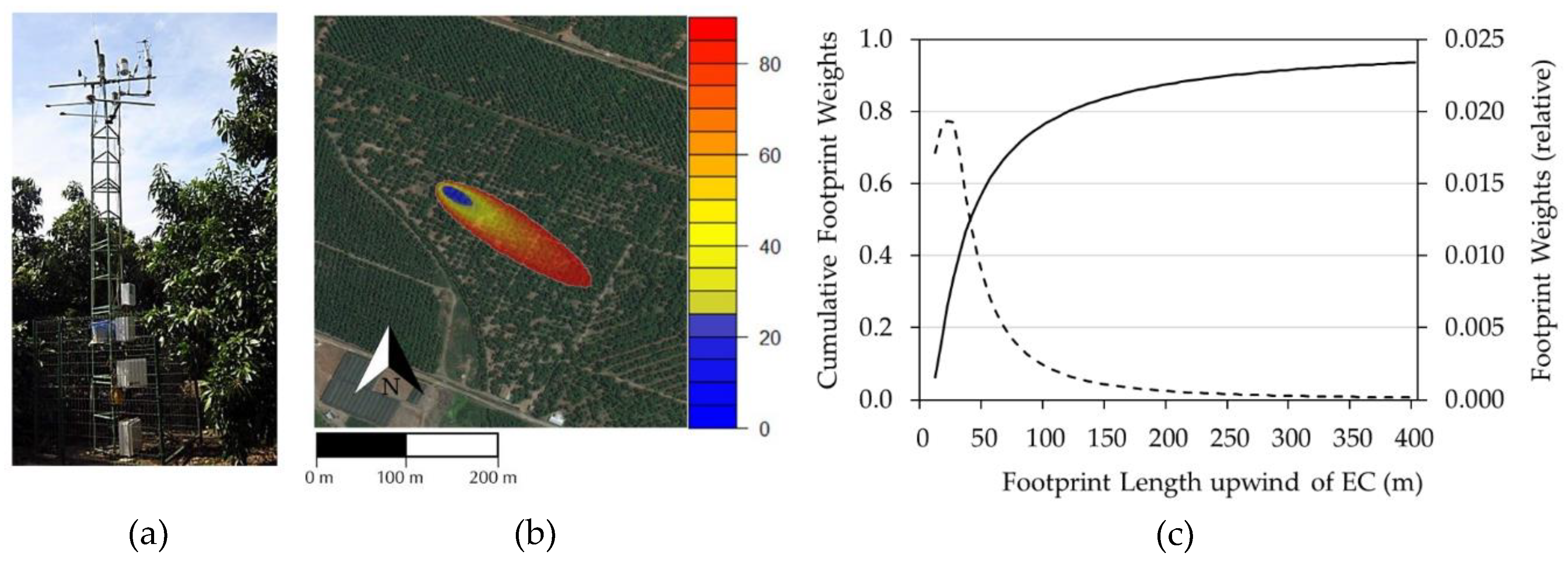
2.1. Study Site

The trial was implemented in a commercial avocado orchard between spring and summer of the 2013–2014 season. The orchard is located in the Aconcagua Valley, Valparaíso Region, Chile (32°48′33.40″ LS, 71°14′16.86″ LW, 182 m.a.s.l.). The orchard (35 years-old) was planted in rows facing northwest at 10 × 10 m (100 plants ha−1). The average canopy height was around of 4.9 m. Using the MODIS/Terra Leaf Area Index product version 6 provided by the United States Geological Survey (USGS) (https://lpdaac.usgs.gov/), the leaf area index (LAI) was estimated during the study period (10 satellite images), the resulting average value was 1.85 m2 m−2 with and standard deviation of ±0.31 m2 m−2.
The climate in the study site is warm temperate with dry and warm summers (Köppen climatic classification: Csb) with 14.4 °C of daily average temperatures and 457 mm of average annual rainfall [21]. The dry period extends approximately for 8 months. Summer is usually hot and dry, registering only 4.6% of annual rainfall. 13.1% of the rainfall of the year occurs in spring, 56% is concentrated in winter, and 26.3% in autumn. The soil of the field is classified as Quillota clay loam series (QLT), “Fine, mixed, thermal Typic Xerumbrepts (Inceptisol)” [22]. The experimental plot of 3.2 ha is surrounded by other avocado crops (total 20 ha) under the same conditions and agronomic management (Figure 1b). The flat surface (slope less than 2%) is homogeneously covered by the crop. The soil remained free of weeds and other crops during the study period. The orchard was daily irrigated during spring–summer (October to March), and every 4 days in the autumn–winter period (April to September) by micro-sprinkler system, according to the water requirements estimations suggested by the National Agricultural Research Institute of Chile (INIA—Instituto de Investigaciones Agropecuarias) (https://www.inia.cl/) [23]. Total seasonal irrigation in the study area was 1400 mm year−1 (14,000 m3 ha−1 year−1).

2.2. Measurement of Energy Balance Components

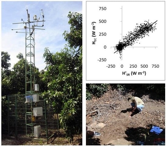
2.2.1. Turbulent Fluxes Measurements (H and LE)

H and LE were measured with an EC system mounted on a 6 m high metal tower (1 m over the canopy), oriented in the dominant wind direction (West) (Figure 1a). EC measures the vertical wind transport from the surface using an averaged sonic temperature over a period of time [26,27] and assumes that the vertical heat flux corresponds to the total heat flux. Then, it obtains H and LE based on the determination of the covariance between scalar fluctuations in vertical wind speed (w), air temperature (T), and water vapor [28]. Following this principle H and LE are estimated using the Equations (1) and (2):
H E C = ρ × C p × w T ¯
L E E C = λ × w q ¯
where HEC is the sensible heat flux (W m−2), LEEC is the latent heat flux (W m−2), ρ is the water vapor density (kg m−3), λ is the latent heat of vaporization (J kg−1), Cp is the specific heat capacity of air at constant pressure (J kg−1 °C−1), w is the fluctuation on the vertical wind speed (m s−1), T is the fluctuation in the air temperature (°C), and q’ is the fluctuation in the water vapor density (kg m−3) [29,30,31,32,33]. The EC system used in this study consisted on a 3D sonic anemometer (Windmaster Pro, Gill Instruments, Hampshire, UK) and an open path gas analyzer of CO2/H2O (OP-2, ADC Bioscientific Ltd., Hoddesdon, UK). The footprint analysis was implemented by a one-dimensional model [25] and a two-dimensional model [24], using a MATLAB code (version 2019a) and the R-Package “FREddyPro” [34], respectively. The peak footprint location (xmax) was about 18 m for a typical day under unstable conditions (Figure 1c). The cumulative normalized flux (CNF) measurements of 90% were around 200 m (Figure 1b).
The frequency of measurements was 10 Hz averaged over 30 min. Data were recorded on a datalogger (CR1000, Campbell Scientific Inc., Logan, Utah, USA). The processing of data and corrections were done with the software Eddysoft (Meteotools, Max Planck Institut für Biochemie, Martinsried, Germany).

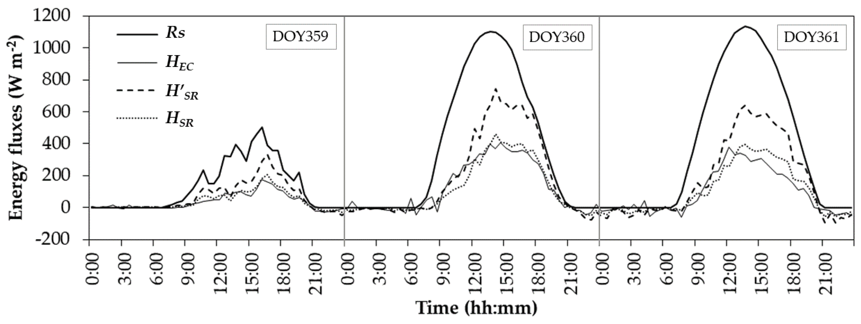
2.2.2. Measurements of Net Radiation (Rn) and Soil Heat Flux (G)

Net radiation (Rn) was measured with a net radiometer (NR2, Delta-T Devices, Cambridge, UK) installed on the EC tower. Two soil heat flux plates (HFP01, Hukseflux Thermal Sensors, Delft, The Netherlands) at 7 cm depth, one over the row at 3.5 m from the tower and the other in the next row, were used to determine G. The absorption or liberation of heat in the soil above the plates was measured using four copper-constantan thermocouples; two above the row and two in the next row, at 2 and 6 cm depth, which measured the variation in soil temperature.

2.3. Evaluation of the Energy Balance Closure (EBC)

The surface energy balance relates Rn, LE, H, and G, as follows in Equation (3):
R n = L E + H + G
EC allows to accurately measure H and LE, however is important to evaluate the quality of these measures. In this context, the closure of the energy balance equation is used to evaluate the EC measurements [35] and should be evaluated before using HEC to calibrate H’SR. Thus, to evaluate the quality of the data, a linear regression between the sum of the turbulent flows (LEEC + HEC) and the available energy (Rn − G) [36,37] was constructed on a half-hourly basis. Then, it is possible to calculate EBR (energy balance ratio, dimensionless), which corresponds to the proportion of turbulent flows over the available energy [9], Equation (4):
E B R = H E C + L E E C R n G
The use of a tolerance range for EBR values between 0.8 and 1.2 (±20% tolerance) [38], allows to ensure a set of reliable data measured with EC to be able to calibrate SR.
The final dataset includes spring and summer measurements between October 18, 2013 (DOY-day of year 291) and December 31, 2013 (DOY 365). From the point of view of the water requirements, during this spring–summer (October–March) period, the most critical events occur simultaneously in the development of the avocado, sprouting, flowering, root growth and fruit set [23]. Additionally, from a climatic point of view, in the region of the study site this particular period presents a higher variability in the climatic conditions, which was desirable for the proposed analysis. According to [21], average wind speed is between 2.0 y 2.7 m s−1 usually southwest and average temperatures vary between 9.9 and 25.5 °C.

2.4. Surface Renewal Method (SR)

SR method is based on the theory of coherent structures [30], which allows describing the variation of the temperature measured at high frequency on a canopy when a parcel of air moves toward the surface [31,32]. The energy transfer between air and canopy heats or cools the air on the surface, then the air parcel is displaced from the surface and replaced by another from ground to top [9,32,33].
To evaluate the potential of SR utility, high frequency (10 Hz) temperature values were recorded with a fast E-type thermocouple (0.076 mm diameter) (FW03, Campbell Scientific Inc., Logan, UT, USA) installed at 6 m of height in the same tower with EC equipment. The dataset was recorded and processed with a datalogger (CR1000, Campbell Scientific Inc., Logan, UT, USA), and stored in a compact 2.0 Gb flash memory card, and then manually transferred to a personal computer.
The structure-function of the air temperature data was used to determine the parameters describing the ramp: the amplitude (A) and the frequency (τ), for stable and unstable atmospheric conditions [9,12,14]. The estimated H values with the uncalibrated SR method (H’SR) was calculated according to Equation (5), with an algorithm implemented directly in the datalogger [14,32]:
H S R = ρ × C p × ( A τ ) × z
where ρ and Cp are the density and the specific heat of the air at constant pressure, respectively. The value A corresponds to the amplitude or increase of temperature in the air parcel; A is positive when the atmosphere is unstable, therefore H is positive when the flux rises. The parameters of the ramp, A and τ were determined using the structure-function analysis method [30].

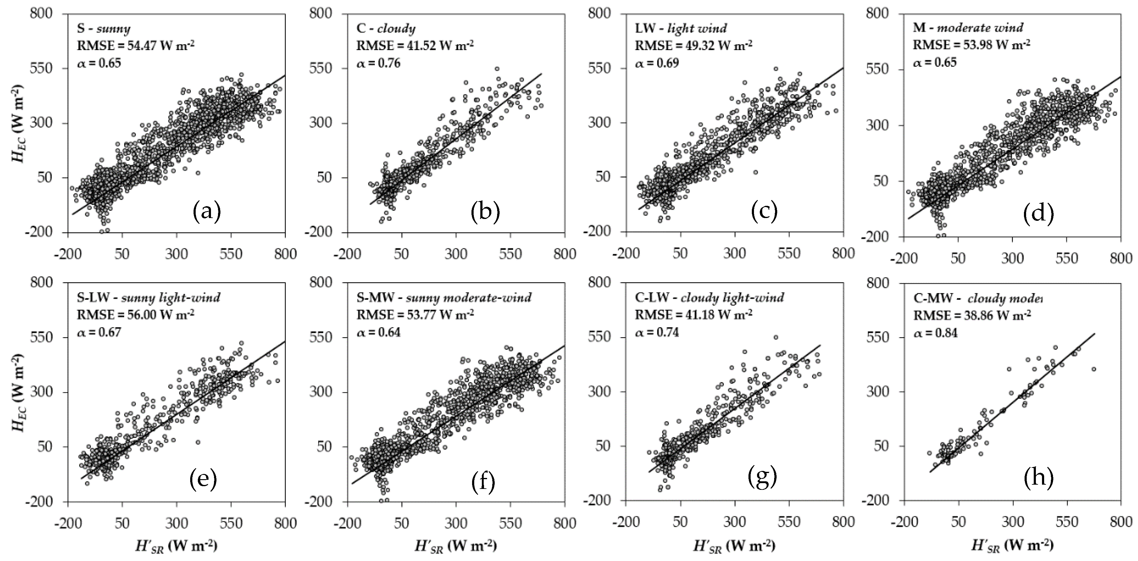
2.5. Meteorological Categories

2.5.1. Categorization by Wind Condition

The atmospheric boundary layer is a space adjacent to the earth’s surface, in which surface friction has a considerable effect on the flow of air parcels, which generates important changes in temperature, wind, and depth of this layer during the course of the day [39]. When the air on evaporating surfaces is not constantly removed by drier air, the surrounding water vapor is maintained, and the evapotranspiration rate is reduced. Under wind conditions, the air is removed, and the new parcel of dry air must again be saturated, favoring the evapotranspiration rate [6].
The Beaufort wind scale has been widely used to empirically measure wind intensity based on the description of its effects, initially on the sea. It has now been adapted to terrestrial use and, in particular, to describe the effect of wind on vegetation [40]. On this scale, the wind force is categorized descriptively from calm wind to hurricane, which is numerically represented in levels from 0 to 12 [41,42,43]. Level 2 or light breeze (1.7–3.0 m s−1) is the first category of this scale that refers to the effect on vegetation, which is described as “light leaf movement.”
Wind speed data were obtained from the meteorological station of La Cruz city [44] located 1600 m at the south-east direction of the study site. Wind speed records from La Cruz station were available in average measurements (m s−1) every hour, these values were compared with the wind speed measurements obtained at the study site. During the study period, both stations presented very similar trends and amounts. Since the average of the time records could mask certain wind speed data (for example, sudden gusts of wind on a calm day), the procedure used to perform this classification was based on counting the number of hours per day in which the wind did not exceed level 1 of the Beaufort scale. In this way, the percentage of hours per day when the wind reaches Beaufort level 1 can be obtained, and the percentage of hours in which the wind is equal to or above Beaufort level 2. Then, if one day presents more than 50% of its hours with winds greater than or equal to level 2, is categorized as Moderate Wind (MW, 37 days), otherwise, it is categorized as Light Wind (LW, 28 days).

2.5.2. Categorization by Solar Radiation (Sunny and Cloudy Days)

The whole data set (3120 half-hours equivalent to 65 days) was classified on sunny and cloudy days. To do this, an adaptation of the methodology proposed by [45] was used, which defines a KT index—Equation (6)—that relates the incoming solar radiation (Rs) and the extra-terrestrial radiation (Ra):
K T = R s R a
Rs values were obtained from a pyranometer installed in the EC and SR sensor tower, connected to the same datalogger. The Ra values were obtained from [6] considering the latitude of the experimental site.

2.6. Calibration Factor Alpha (α)

The SR method allows estimating H according to the variation of the temperature of the localized and immediately exchanged air parcels inside the crop canopy. Thus, the morphological characteristics of the species and consequent heterogeneous distribution of heat sources within the canopy cause that these air parcels describe uneven heating [12,14,26]. In this way, there are methodological and procedural differences between EC and SR to obtain their results, after which [13] emphasizes that the estimates of the surface renewal method must be calibrated against EC data to explain the lack of uniformity or bias that presents the heating of the air parcels, and thus correct the existence of overestimation or underestimation of H by the calibration factor α.
For all meteorological categories (9 conditions; 8 categories plus the whole dataset) α was estimated by simple linear regressions forced through the origin between H’SR and HEC, Equation (7). This analysis was performed for the data recorded every half-hour and for the daily accumulated data. The slopes of the regression lines correspond to the α values for each condition:
H S R = α × H S R
where HSR is the calibrated value of sensible heat flux and H’SR is the raw value of sensible heat flux obtained by SR.

2.7. Statistical Analysis

All calibration factors α for the conditions analyzed in this study were obtained by means of a linear regression analysis between H’SR and HEC. The regressions were forced through the origin (intercept equal to zero) to obtain only the value of the slope, which represents the calibration factor α (7). The linear regression analyses were implemented in R software version 3.2.5 [46] using the linear function “lm-linear model”. The graphical representation of the regressions was done using the package “ggplot2” [47] including 95% confidence intervals for slope values. Once α values were calculated, the statistical analysis to compare the observed and estimated values of H consisted in determining the root mean square error (RMSE) and the mean absolute error (MAE) [48,49]. This analysis was applied to each of the nine categories, both for the case in which fixed α-value was used with hourly and daily data and for when variable α-value was used for hourly and daily data. Finally, to compare the slopes (α values) of the different meteorological conditions, a t-test was implemented with a level of significance of 5%.

3. Results and Discussion

3.1. Meteorological Categories

During the study period, daily mean Ra values were 37.1, 42.0, and 44.1 (MJ m−2 day−1) in October, November, and December, respectively. Regarding data recorded every half-hour, it should be noted that the daily average values of Rs and Rn for sunny days were 352.9 W m−2 and 214.2 W m−2, respectively. For cloudy days, these values were 207.3 W m−2 and 132.7 W m−2. Maximum values of solar and net radiation were recorded around noon with 1292.0 W m−2 and 827.0 W m−2 for sunny days and 1366.2 W m−2 and 867.0 W m−2 for cloudy days, respectively. These data show a slight rise in the maximum radiation of the cloudy days over sunny days, which could be explained by the capture of sensor data when the sun’s rays pass through weak or zero cloudiness. After the solar radiation categorization, the classification of the 65 days of the study resulted in the division presented in Table 1.
The final classification of the dataset was made according to solar radiation and wind conditions together. Eight meteorological categories plus the whole dataset were established to perform analyses and comparisons: (1) Whole dataset (WD), (2) sunny (S), (3) cloudy (C), (4) light wind (LW), (5) moderate wind (MW), (6) sunny light-wind (S-LW), (7) sunny moderate-wind (S-MW), (8) cloudy light-wind (C-LW), and (9) cloudy moderate-wind (C-MW).

3.2. The Effect of the Alpha Value in the Estimation of the Sensible Heat Flux

The traditional method to obtain α implies the use of the EC system to measure H, and thus generate the regression line forced through the origin against the uncalibrated H values estimated with SR. It is then possible to obtain H calibrated with α to finally estimate LE using the equation of surface energy balance (3) [9,12,14]. Figure 2 shows an example of the effect of α in the determination of H, (daily pattern) for three consecutive days: a cloudy day (DOY 359) and two sunny days (DOY 360 and 361) (Solar radiation was included in the figure). In general, the uncalibrated values of H (H’SR) are higher than the measured, therefore, α factor must be applied to adjust the fluxes. From the figure, it is very evident that the use of the α factor allows correcting the sensible heat flux showing a good adjustment in the amounts and hourly variations.
According to Hu et al. [10], in most cases, researchers have classified the data set according to atmospheric stability conditions. In this way, on the one hand, the negative H values registered mainly during the night hours are grouped, when there is atmospheric stability, and on the other, the positive values registered during the day are grouped, when conditions of atmospheric instability appear. Then, a single value α—under atmospheric instability—is obtained, which is used in the final calculations of ETa. Several studies have described that α depends on several factors. Differences in α were presented when data were separated under stable (s) and unstable (us) in maize, walnut, and forest [12]. A similar effect was reported in a peach orchard [35]. The dependence of α on the height of the sensor was stated on avocado canopy [15] and in vineyards [18]. The configuration of the thermocouple can also play a role in the determination of α, Snyder and O’Connell [50] obtained different α values for the same crop in two growing seasons using different thermocouple configurations. Castellví et al. [51] determined α for 3 periods of 15 days in a year for stable and unstable conditions with the sensor installed at two heights. From this study differences in the calibration factor suggest that α should be obtained continuously throughout the year. The SR analysis proposed by Poblete-Echeverría et al. [52] was done considering different phenological periods through the growing cycle of a vineyard, to obtain the calibration factor with the sensor located at different heights, which determined a range of α values for this variation and the phenological stages.
The α factor is proportional to the energy presented in the system. In the SR method, the determination of HSR depends on A and τ that characterizes temperature ramps (5). When sunny and cloudy days were compared according to these parameters no differences were registered in τ, both conditions presented similar values with average around 15 s during daily hours (8:00 to 18:00). However, substantial differences were registered in A. In sunny days, A reached maximum values around 3 °C, while on cloudy days the maximum values were around 0.5 °C. Lower A values on cloudy days indicates less energy and therefore the correction factor needs to be higher to compensate for this effect. α values for cloudy days were consistently higher for all analyzed dates. In the 30-min approach, the α value calculated from the cloudy days was 17% higher than that estimated from sunny days. A similar tendency was registered in the daily approach.

3.3. Estimation of HSR With a Fixed Alpha Value

In order to quantify the effect (error) of applying a fixed alpha value for each meteorological condition, RMSE and MAE were calculated. Table 2 shows three situations: (a) Where the traditional methodology was used to determine α from the data recorded every half-hour (α = 0.66); (b) using the same value obtained in (a) (α = 0.66) to calculate daily accumulated HSR; and (c) using α obtained from the daily accumulated values (α = 0.73) to calculate daily HSR. According to Table 2(a), the RMSE value obtained in this study for the whole data set (RMSE = 52.25 W m−2) is similar to the values indicated by other authors using a fixed α value. When this fix value is used in the deferent categories the RMSE fluctuated between 43.49 W m−2 (C-LW condition) and 54.66 W m−2 (S condition). Literature shows that the best estimate of H in avocado was α = 0.59, which considered half-hour periods (n = 40) for its determination (RMSE = 36 W m−2) [15]. On the other hand, three α calibration factors were determined according to three periods within one year under unstable atmospheric conditions: 0.66 (n = 304), 0.58 (n = 271) and 0.76 (n = 183) [51]. In this case the RMSE values reported were 61, 75, and 51 W m−2, respectively.
In a practical way, the accumulated data are those that are usually used for the estimation of evapotranspiration in a daily basis (mm day−1). Therefore, we also proceeded to determine and compare the accumulated daily HSR and HEC values, first using the same calibration factor α obtained with the complete data set every half-hour, that is, before obtaining daily data (Table 2(b)), and using the accumulated data set to obtain a new calibration factor α, that is, α after obtaining daily data (Table 2(c)). The results indicate that, for all datasets, better estimates were obtained when determining calibration factor α after performing the accumulation data (Table 2(c)), that is with α = 0.73, with α from each half-hour data (Table 2(b)). This could be because the procedure of accumulating daily data subtracts the negative values of H measured during the night and presents a real value of the energy that accumulates in the form of sensible heat during a whole day and not that of instants each half-hour. For example, with α = 0.66 RMSE of WD is 1.50 MJ m−2 day−1, while with α = 0.73, RMSE of WD is 1.22 MJ m−2 day−1.

3.4. Estimation of HSR with Variable Alpha Values

Alternatively, to the use of a fixed α value to calculate HSR, it is possible to determine a single calibration factor for each meteorological condition and thus establish if there are significant differences between them. Table 3 shows the α values and their respective coefficients of determination obtained when the categorization was previously carried out according to weather conditions. As was presented in Table 2, Table 3 shows three situations, but in this case for each meteorological condition: (a) Alphas calculated with the traditional method (data set by condition every half-hour); (b) the same alphas calculated in (a) but applied to the daily accumulated data; and (c) alphas calculated from the daily accumulated data. In Table 3(a) there are three categories that stand out for presenting calibration factors greater than the other categories: cloudy, cloudy light-wind, and cloudy moderate-wind, with α = 0.76, α = 0.74, and α = 0.84, respectively, situation that is repeated with the same categories in (c) where α = 0.79 for C, α = 0.77 for C-LW and α = 0.90 for C-MW. In Table 3 there are no changes since the same α values were used as in (a). As when comparing Table 3(b) with Table 3(c), RMSE in Table 3(c) represent better estimates of HSR than Table 3(b), since all RMSE for each of the meteorological categories are less or equal. Thus, categorization by meteorological conditions and usage of accumulated energy allows estimating HSR with better precision. Likewise, it is possible to conclude that cloudiness alone and combined with any wind category, strongly affects α, increasing its value, which implies that HSR subtracts more energy from the system under these conditions.
Figure 3 shows the results of the method (linear regression) used to obtain the α value for each condition. When the conditions are compared, some changes in the slopes (α value) and dispersion are evident, especially for cloudy conditions (Figure 3g,h).
In Poblete-Echeverría et al. [52] H’SR and HEC were recorded every 15 minutes during one season in a vineyard, so they were able to estimate HSR with RMSE 52.2 W m−2 and MAE 35.2 W m−2. When they analyzed the daily dataset, they were able to estimate HSR with a RMSE of 0.80 MJ m−2 day−1 and MAE of 0.67 MJ m−2 day−1. Also, in vineyard, Poblete-Echeverria and Ortega-Farias [20], estimated HSR with a RMSE of 38.0 and MAE 26.0 W m−2. These two studies provide estimates of HSR with similar adjustments to those found in avocado. In addition, both studies were performed under similar phenological stages on spring–summer period in semi-arid climatic conditions, which allows the comparison between deciduous (vine) and persistent (avocado) species results, at the moment when both have foliar coverage. It should be noted that, in this study, there was no separation of data regarding the phenological stages of the avocado trees since avocado maintains a rather uniform foliar coverage during its whole cycle. Thus, plant architecture and rugosity surface that measurements faced, would not be determining factors during the study period.
Comparing RMSE in Table 2(a) and Table 3(a), the latter is lower or equal, indicating that the HSR estimates are better when the meteorological categorization was performed, compared to the fixed α method from the whole dataset. When comparing (b) and (c) in Table 2 with (b) and (c) in Table 3, the estimation of HSR is better when accumulated energy data H’SR and HEC is used before calculating α. In this way, α is determined directly from the daily accumulated data (MJ m−2 day−1). It should be noted that S, MW, and S-MW categories are the only ones that reflect slightly unfavorable values when comparing RMSE between fixed and variable α (Table 2(b) and Table 3(b)). This situation could be explained by the considerable increase in α value for each of these meteorological conditions with respect to α = 0.66 fixed.
Table 3 showed the calculated alpha values for each meteorological condition and its consequent effect on the estimation of HSR, which can be tested by different RMSE and MAE values obtained. However, to establish the significance of these differences, pairs of α values were analyzed. Table 4 shows a comparison between all variable α values. When WD is analyzed (α = 0.66) and compared with the other categories, α shows significant differences compared to 7 of the 8 conditions. For S-LW it is not possible to ensure the existence of differences compared to WD (p-value > 0.05). However, it is relevant to identify and separate data set under sunny (S) and cloudy (C) days conditions, using solar radiation as the main factor, as well as on days with light wind (LW) and moderate (MW), with the objective of establishing an accurate α value. From the point of view of cloudiness, the category S (α = 0.65) shows significant differences when compared with C (α = 0.76), LW (α = 0.69), C-LW (α = 0.74), and C-MW (α = 0.84), which implies that α is different between S and any cloudiness condition, even with light or moderate wind. For condition C (α = 0.76), α is different from all other categories except C-LW (α = 0.74), which would indicate that a cloudy day with light wind is not sufficiently different from a day classified as cloudy for determining alpha. Regarding wind condition, LW (α = 0.69) is different to all the other categories, which indicates that the presence of light wind does affect α and it is relevant to perform this classification to obtain this factor. However, the MW category (α = 0.65) turned out to be significantly different only for days C (α = 0.76), LW (α = 0.69), C-LW (α = 0.74) and C-MW (α = 0.84). It should be noted that under the combined meteorological conditions S-LW (α = 0.67), S-MW (α = 0.64), C-LW (α = 0.74), and C-MW (α = 0.84), there were clear differences of S -LW and S-MW against any cloud condition, even with light or moderate wind. C-LW showed no differences with C. While C-MW showed differences in all meteorological conditions.

4. Conclusions

The calibration of the SR method under different meteorological conditions was done by a meteorological classification based on solar radiation and wind intensity. From the comparison between half-hour values versus daily values the best results were obtained using an α obtained from daily H’SR. The α-values obtained each meteorological condition (α variable) were compared and evaluated to determine the effect of the use of a variable and fixed value of α in the estimation of H. The results show that α varies according to meteorological conditions. Significant differences were found between meteorological classes especially under cloudy conditions accompanied by light or moderate wind. The effect of the wind is evident when comparing α in light wind days against any other meteorological categorization. However, the effect of moderate wind is mainly relevant for days with cloudiness.
Further studies are needed for identifying differences between the calibration factors for different categories with prevailing cloudiness, as well as between the different ranges of winds described by the Beaufort scale, and thereby establishing under what meteorological conditions it is really pertinent to determine and modify alpha, for the estimation of H using the SR method.

Author Contributions

Conceptualization, C.P.-E. and R.F.; methodology, A.M. and C.P.-E.; formal analysis, A.M. and C.P.-E.; writing—original draft preparation, A.M.; writing—review and editing, C.P.-E.; data curation, A.M.; supervision, R.F., G.S., E.S., A.C.-M., and C.P.-E.; project administration, R.F., G.S., and C.P.-E. All authors have read and agreed to the published version of the manuscript.

Funding

This research was funded by the National Commission for Scientific and Technological Research CONICYT (FONDECYT de Iniciación N° 11130601).

Conflicts of Interest

The authors declare no conflict of interest.

References

  1. Holzapfel, E.; De Souza, J.A.; Jara, J.; Carvallo, H. Responses of avocado production to variation in irrigation levels. Irrig. Sci. 2017, 35, 205–215. [Google Scholar] [CrossRef]
  2. Lahav, E.; Kalmar, D. Determination of the Irrigation Regimen for an Avocado Plantation in Spring and Autumn. Aust. J. Agric. Res. 1983, 34, 717–724. [Google Scholar] [CrossRef] [Green Version]
  3. Lahav, E.; Whiley, A.W.; Turner, D.W. Irrigation and Mineral Nutrition. In The Avocado Botany, Production and Uses, 2nd ed.; Schaffer, B., Wolstenholme, B.N., Whiley, A.W., Eds.; CAB International: Croydon, UK, 2013; pp. 301–341. ISBN 978 1 84593 701 0. [Google Scholar]
  4. Neuhaus, A.; Turner, D.W.; Colmer, T.D.; Kuo, J.; Eastham, J. Drying half the root-zone of potted avocado (Persea americana Mill., cv. Hass) trees avoids the symptoms of water deficit that occur under complete root-zone drying. J. Hortic. Sci. Biotechnol. 2007, 82, 679–689. [Google Scholar] [CrossRef]
  5. Ferreyra, R.; Sellés, G.; Burgos, L.; Villagra, P.; Sepúlveda, P.; Lemus, G. Manejo Riego en Frutales en Condiciones de Restricción Hídrica, Boletín INIA nº 214; Instituto Nacional de Investigaciones Agropecuarias: Santiago, Chile, 2010; pp. 65–72. ISSN 0717-4829. [Google Scholar]
  6. FAO. Evapotranspiración del Cultivo. Guías para la Determinación de Los Requerimientos de Agua de Los Cultivos; Food and Agriculture Organization: Roma, Italy, 2006; pp. 1–79. ISBN 92-5-304219-2. [Google Scholar]
  7. Katerji, N.; Rana, G. FAO-56 methodology for determining water requirement of irrigated crops: Critical examination of the concepts, alternative proposals and validation in Mediterranean region. Theor. Appl. Climatol. 2013, 116, 515–536. [Google Scholar] [CrossRef]
  8. Zapata, N.; Martínez-Cob, A. Estimation of sensible and latent heat flux from natural sparse vegetation surfaces using surface renewal. J. Hydrol. 2001, 254, 215–228. [Google Scholar] [CrossRef] [Green Version]
  9. Zapata, N.; Martínez-Cob, A. Evaluation of the surface renewal method to estimate wheat evapotranspiration. Agric. Water Manag. 2002, 55, 141–157. [Google Scholar] [CrossRef] [Green Version]
  10. Hu, Y.; Buttar, N.A.; Tanny, J.; Snyder, R.L.; Savage, M.J.; Lakhiar, I.A. Surface Renewal Application for Estimating Evapotranspiration: A Review. Adv. Meteorol. 2018, 2018, 1–11. [Google Scholar] [CrossRef] [Green Version]
  11. López-Olivari, R.; Ortega-Farías, S.; Poblete-Echeverría, C. Energy balance components and evapotranspiration measurements over a superintensive olive orchard. Int. Symp. Irrig. Hortic. Crops 2007, 1150. [Google Scholar] [CrossRef]
  12. Qiu, J.; Su, H.B.; Watanabe, T.; Brunet, Y. Surface renewal analysis: A new method to obtain scalar fluxes. Agric. For. Meteorol. 1995, 74, 119–137. [Google Scholar] [CrossRef]
  13. Spano, D.; Snyder, R.L.; Duce, P. Surface renewal analysis for sensible heat flux density using structure functions. Agric. For. Meteorol. 1997, 86, 259–271. [Google Scholar] [CrossRef]
  14. Snyder, R.L.; Spano, D.; Pawu, K.T. Surface renewal analysis for sensible heat and latent heat flux density. Bound. -Layer Meteorol. 1996, 77, 249–266. [Google Scholar] [CrossRef]
  15. Spano, D.; Duce, P.; Snyder, R.L.; Paw, U.K.T. Surface renewal estimates of evapotranspiration. Tall canopies. Int. Symp. Irrig. Hortic. Crops 1997, 449, 63–68. [Google Scholar] [CrossRef]
  16. Chen, W.; Novak, M.D.; Black, T.A.; Lee, X. Coherent eddies and temperature structure functions for three contrasting surfaces. Part II: Renewal model for sensible heat flux. Bound. -Layer Meteorol. 1997, 84, 125–147. [Google Scholar] [CrossRef]
  17. Duce, P.; Spano, D.; Snyder, R.L.; Paw, U.K.T. Surface renewal estimates of evapotranspiration. Short canopies. Int. Symp. Irrig. Hortic. Crops 1997, 449, 57–62. [Google Scholar] [CrossRef]
  18. Spano, D.; Snyder, R.L.; Duce, P. Estimating sensible and latent heat flux densities from grapevine canopies using surface renewal. Agric. For. Meteorol. 2000, 104, 171–183. [Google Scholar] [CrossRef]
  19. Castellví, F. Combining surface renewal analysis and similarity theory: A new approach for estimating sensible heat flux. Water Resour. Res. 2004, 40, 1–20. [Google Scholar] [CrossRef] [Green Version]
  20. Poblete-Echeverria, C.; Ortega-Farias, S. Estimation of vineyard evapotranspiration using the surface renewal and residual energy balance methods. Int. Symp. Irrig. Hortic. Crops 2014, 1038, 633–638. [Google Scholar] [CrossRef]
  21. Santibáñez, F.; Uribe, J. Atlas Agroclimático de Chile, Regiones V y Metropolitana; Universidad de Chile: Santiago, Chile, 1990; pp. 3–65. [Google Scholar]
  22. CIREN. Descripciones de Suelo, Materiales y Símbolos. Estudio Agrológico V Región, Tomo 2; Publicación 116; Centro de Información de Recursos Naturales: Santiago, Chile, 1997. [Google Scholar]
  23. Lemus, G.; Ferreyra, R.; Gil, P.; Maldonado, P.; Toledo, C.; Barrera, C.; de Celedón, A.J.M. El Cultivo del Palto, Boletín INIA nº 129; Instituto de Investigaciones Agropecuarias: La Cruz, Chile, 2005; pp. 53–64. ISSN 0717-4829. [Google Scholar]
  24. Kormann, R.; Meixner, F. An analytical footprint model for non-neutral stratification. Bound. -Layer Meteorol. 2001, 99, 207–224. [Google Scholar] [CrossRef]
  25. Hsieh, C.; Katul, G.; Chi, T. An approximate analytical model for footprint estimation of scaler fluxes in thermally stratified atmospheric flows. Adv. Water Resour. 2000, 23, 765–772. [Google Scholar] [CrossRef]
  26. Shapland, T.M.; Snyder, R.L.; Smart, D.R.; Williams, L.E. Estimation of actual evapotranspiration in winegrape vineyards located on hillside terrain using surface renewal analysis. Irrig. Sci. 2012, 30, 471–484. [Google Scholar] [CrossRef]
  27. Burba, G. Eddy Covariance Method for Scientific, Industrial, Agricultural, and Regulatory Applications; LI-COR® Biosciences: Lincoln, NE, USA, 2013; pp. 7–30. ISBN 978-0-615-76827-4. [Google Scholar]
  28. Balbontín–Nesvara, C.; Calera-Belmonte, A.; González-Piqueras, J.; Campos–Rodríguez, I.; Llanos López-González, M.; Torres-Prieto, E. Comparación de los sistemas covarianza y relación de Bowen en la evapotranspiración de un viñedo bajo clima semi–árido. Agrociencia 2011, 45, 87–103. [Google Scholar]
  29. Abraha, M.G. Sensible Heat Flux and Evaporation for Sparse Vegetation Using Temperature-Variance and a Dual-Source Model. Ph.D. Thesis, University of KwaZulu-Natal, Pietermaritzburg, South Africa, 2010. [Google Scholar]
  30. Van Atta, C.W. Effect of coherent structures on structure functions of temperature in the atmospheric boundary layer. Arch. Mech. Stosow. 1977, 29, 161–171. [Google Scholar]
  31. Gao, W.; Shaw, R.H. Observation of organized structure in turbulent flow within and above a forest canopy. Bound. -Layer Meteorol. 1989, 47, 349–377. [Google Scholar] [CrossRef]
  32. Snyder, R.L.; Paw, U.K.T.; Spano, D.; Duce, P. Surface renewal estimates of evapotranspiration. Theory. Int. Symp. Irrig. Hortic. Crops 1997, 449, 49–55. [Google Scholar] [CrossRef]
  33. McElrone, A.J.; Shapland, T.M.; Calderon, A.; Fitzmaurice, L.; Snyder, R.L. Surface Renewal: An Advanced Micrometeorological Method for Measuring and Processing Field-Scale Energy Flux Density Data. JoVE (J. Vis. Exp.) 2013, 82, e50666. [Google Scholar] [CrossRef] [PubMed] [Green Version]
  34. Xenakis, G. FREddyPro: Post-Processing EddyPro Full Output File. r package version 1.0. 2016. Available online: https://CRAN.Rproject.org/package=FREddyPro (accessed on 1 April 2020).
  35. Castellví, F.; Snyder, R.L. Sensible heat flux estimates using surface renewal analysis. A study case over a peach orchard. Agric. For. Meteorol. 2009, 149, 1397–1402. [Google Scholar] [CrossRef]
  36. Twine, T.E.; Kustas, W.P.; Norman, J.M.; Cook, D.R.; Houser, P.R.; Meyers, T.P.; Prueger, J.H.; Starks, P.J.; Wesely, M.L. Correcting eddy-covariance flux underestimates over a grassland. Agric. For. Meteorol. 2000, 103, 279–300. [Google Scholar] [CrossRef] [Green Version]
  37. Wilson, K.; Goldstein, A.; Falge, E.; Aubinet, M.; Baldocchi, D.; Berbigier, P.; Bernhofer, C.; Ceulemans, R.; Dolman, H.; Field, C.; et al. Energy balance closure at FLUXNET sites. Agric. For. Meteorol. 2002, 113, 223–243. [Google Scholar] [CrossRef] [Green Version]
  38. Poblete-Echeverria, C.; Ortega-Farias, S. Estimation of actual evapotranspiration for a drip-irrigated Merlot vineyard using a three-source model. Irrig. Sci. 2009, 28, 65–78. [Google Scholar] [CrossRef]
  39. Essa, K.S.M.; Embaby, M.M.; Kozae, A.M.; Mubarak, F.; Kamel, I. Estimation of Seasonal Atmospheric Stability and Mixing Height by Using Different Schemes. In Proceedings of the VIII Radiation Physics & Protection Conference, Fayoum, Egypt, 13–15 November 2006. [Google Scholar]
  40. Cullen, S. Trees and wind: Wind scales and speeds. J. Arboric. 2005, 28, 237–242. [Google Scholar]
  41. RMETS. Available online: https://www.rmets.org/weather-and-climate/observing/beaufort-scale (accessed on 28 February 2018).
  42. NOAA. Available online: http://www.spc.noaa.gov/faq/tornado/beaufort.html (accessed on 28 February 2018).
  43. NWS. Available online: http://w1.weather.gov/glossary/index.php?letter=b (accessed on 28 February 2018).
  44. AGROMET. Available online: http://agromet.inia.cl/ (accessed on 21 December 2017).
  45. Rivero, M.; Orozco, S.; Sellschopp, F.S.; Loera-Palomo, R. A new methodology to extend the validity of the Hargreaves-Samani model to estimate global solar radiation in different climates: Case study Mexico. Renew. Energy 2017, 114, 1340–1352. [Google Scholar] [CrossRef]
  46. R Core Team. R: A Language and Environment for Statistical Computing; R Foundation for Statistical Computing: Vienna, Austria, 2016. [Google Scholar]
  47. Wickham, H. ggplot2: Elegant Graphics for Data Analysis; Springer-Verlag: New York, NY, USA, 2009; p. 213. ISBN 978-0-387-98141-3. [Google Scholar]
  48. Willmott, C.J. On the validation models. Phys. Geogr. 1981, 2, 184–194. [Google Scholar] [CrossRef]
  49. Mayer, D.G.; Butler, D.G. Statistical validation. Ecol. Model. 1993, 68, 21–32. [Google Scholar] [CrossRef]
  50. Snyder, R.L.; O’Connell, N.V. Crop coefficients for microsprinkler-irrigated clean-cultivated, mature citrus in an arid climate. J. Irrig. Drain. Eng. 2007, 133, 1. [Google Scholar] [CrossRef]
  51. Castellví, F.; Consoli, S.; Papa, R. Sensible heat flux estimates using two different methods based on surface renewal analysis. A study case over an orange orchard in Sicily. Agric. For. Meteorol. 2012, 152, 58–64. [Google Scholar] [CrossRef]
  52. Poblete-Echeverría, C.; Sepúlveda-Reyes, D.; Ortega-Farías, S. Effect of height and time lag on the estimation of sensible heat flux over a drip-irrigated vineyard using the surface renewal (SR) method across distinct phenological stages. Agric. Water Manag. 2014, 141, 74–83. [Google Scholar] [CrossRef]
Figure 1. (a) EC and SR sensors tower in the avocado orchard, (b) two-dimensional footprint plot [24], and (c) one-dimensional footprint plot [25].
Agronomy 10 00730 g001
Figure 2. Example of sensible heat fluxes measured and estimated (uncalibrated and calibrated) for three consecutive days (DOYs 359, 360, 361). Solar radiation (Rs) is included as reference.
Agronomy 10 00730 g002
Figure 3. Linear regressions forced through the origin between H’SR and HEC. (a) Sunny, (b) cloudy, (c) light wind, (d) moderate wind, (e) sunny light-wind, (f) sunny moderate-wind, (g) cloudy light-wind, and (h) cloudy moderate-wind. Axis Y correspond to the sensible heat flux measured by Eddy covariance (HEC) and axis X correspond to the sensible heat flux estimated by the Surface renewal method (H’SR) All units were expressed in W m−2.
Agronomy 10 00730 g003
Table 1. Days categories according to solar radiation conditions.
KT RangesCategoryn (Days)
0.6 < KT ≤ 1.0Sunny47
0.0 < KT ≤ 0.6Cloudy18
KT is an index that relates the incoming solar radiation and the extra-terrestrial—Equation (6)—, n is the number of days under each category.
Table 2. Estimation adjustments between the sensible heat flux measured by Eddy covariance (HEC) and sensible heat flux estimated by the Surface renewal method (HSR = αH’SR), with fixed α for all categories. (a) fixed α = 0.66, (b) daily values using α = 0.66 and (c) daily values using α = 0.73.
(a) 30-min
α = 0.66, r2 = 0.92
(b) Daily
α = 0.66, r2 = 0.92
(c) Daily
α = 0.73, r2 = 0.98
Datasetn
(h.h)
RMSE
(A.C)
MAE
(A.C)
n
(Days)
RMSE
(A.C)
MAE
(A.C)
n
(Days)
RMSE
(A.C)
MAE
(A.C)
WD312052.2536.33651.501.29651.220.95
S225654.6639.53471.491.28471.250.95
C86445.3627.96181.541.34181.140.97
LW134449.6932.31281.631.41281.291.02
MW177654.1139.37371.401.20371.170.91
S-LW62456.0039.12131.961.75131.591.26
S-MW163254.1439.69341.261.09341.090.83
C-LW72043.4926.40151.271.12150.960.80
C-MW14453.7535.7232.472.4631.791.78
A.C represents values after calibration, h.h represents half-hour data, n is the total data analyzed (30-min or days), RMSE is the root mean square error (expressed in W m−2 and MJ m−2 day−1, for 30-min and daily data, respectively), MAE is the mean absolute error (expressed in W m−2 and MJ m−2 day−1, for 30-min and daily data, respectively), r2 is the determination coefficient, and α is the calibration factor for the SR method. WD, S, C, LW, MW, S-LW, S-MW, C-LW and C-MW correspond to whole dataset, sunny, cloudy, light wind, moderate wind, sunny light-wind, sunny moderate-wind, cloudy light-wind and cloudy moderate-wind, respectively.
Table 3. Estimation adjustments of HEC and HSR (HSR = αH’SR), with variable α for each category. (a) α calculated from 30-min values (b) daily values using α calculated from 30-min values, and (c) daily values using α calculated from daily values.
(a) 30-min(b) Daily(c) Daily
Datasetn
(h.h)
αr2RMSE
(A.C)
MAE
(A.C)
n
(Days)
αRMSE
(A.C)
MAE
(A.C)
n
(Days)
αr2RMSE
(A.C)
MAE
(A.C)
WD31200.660.9252.2536.33650.661.501.29650.730.981.220.95
S22560.650.9254.4739.31470.651.621.42470.720.991.250.97
C8640.760.9241.5226.71180.761.030.84180.790.980.990.79
LW13440.690.9249.3232.12280.691.461.23280.750.981.260.94
MW17760.650.9253.9839.19370.651.511.32370.720.991.160.92
S-LW6240.670.9256.0039.12130.671.951.74130.750.981.571.20
S-MW16320.640.9353.7739.29340.641.451.29340.710.991.060.85
C-LW7200.740.9241.1826.03150.740.930.77150.770.980.910.70
C-MW1440.840.9538.8624.9630.840.800.6830.900.990.560.48
A.C represents values after calibration, h.h. represents half-hour data, n is the total data analyzed (30-min or days), RMSE is root mean square error (expressed in W m−2 and MJ m−2 day−1, for 30-min and daily data, respectively), MAE is the mean absolute error (expressed in W m−2 and MJ m−2 day−1, for 30-min and daily data, respectively), r2 is the determination coefficient, and α is the calibration factor for the SR method. WD, S, C, LW, MW, S-LW, S-MW, C-LW and C-MW correspond to whole dataset, sunny, cloudy, light wind, moderate wind, sunny light-wind, sunny moderate-wind, cloudy light-wind and cloudy moderate-wind, respectively.
Table 4. p-values of statistical comparison between α -values for different meteorological conditions.
DatasetWDSCLWMWS-LWS-MWC-LWC-MW
WD-FalseFalseFalseFalseTrueFalseFalseFalse
S0.003-FalseFalseTrueTrueTrueFalseFalse
C<0.001<0.001-FalseFalseFalseFalseTrueFalse
LW<0.001<0.001<0.001-FalseFalseFalseFalseFalse
MW0.0210.680<0.001<0.001-TrueTrueFalseFalse
S-LW0.8680.055<0.0010.0130.110-FalseFalseFalse
S-MW<0.0010.311<0.001<0.0010.1790.011-FalseFalse
C-LW<0.001<0.0010.064<0.001<0.001<0.001<0.001-False
C-MW<0.001<0.001<0.001<0.001<0.001<0.001<0.001<0.001-
Numeric data correspond to p-values obtained when comparing slopes (α -values) between different meteorological conditions. t-test. Null hypothesis was represented by H0: b1 = b2, (b1 and b2 are any pair of slopes to be tested), α = 0.05, CI = 95%. p-value > 0.05 is indicated by True (b1 = b2), p-value ≤ 0.05 is indicated by false (b1 ≠ b2). Self-comparisons were omitted of the analysis (grey cells). WD, S, C, LW, MW, S-LW, S-MW, C-LW and C-MW correspond to whole dataset, sunny, cloudy, light wind, moderate wind, sunny light-wind, sunny moderate-wind, cloudy light-wind and cloudy moderate-wind, respectively.

