Study of C, N, P and K Release from Residues of Newly Proposed Cover Crops in a Spanish Olive Grove

Abstract

Cover crops (CC)s are increasingly employed by farmers in olive groves. Spontaneous soil cover is the most commonly used CC. Its continuous utilization changes ruderal flora. It is necessary to study new CCs. Living CCs provide C and nutrients to soil during decomposition. Information on this issue in olive groves is scarce. A 4-year field study involving grab sampling of Brachypodium distachyon, Sinapis alba and spontaneous CC residues was conducted to study C and nutrient release from cover crop residues. Throughout the decomposition cycles, C, N and P release accounted for 40 to 58% of the C, N and P amounts in the residues after mowing. Most K was released (80–90%). Expressed in kg per hectare, the release of C and N in Brachypodium (C: 4602, N: 181, P: 29, K: 231) and Sinapis (C: 4806, N: 152, P: 18, K: 195) was greater than that in spontaneous CC (C: 3115, N: 138, P: 21, K: 256). The opposite results were observed for K. The Rickman model, employed to estimate the amount of C, N and P in residues, yielded a good match between the simulated and measured values. In comparison to spontaneous CC, the newly proposed CCs have a higher potential to provide soil with C and N.

1. Introduction

The Mediterranean basin accounts for 95% of the global area of olive (Olea europaea L.) trees [1]. It is the main tree species among those cultivated in the Mediterranean area and dominates its rural landscape [2]. Spain has the highest production and surface area in the world, with 2.73 Mha [3], and over 60% of the olive production in the European Union. This production has continued to grow over the last 20 years. Andalusia has 1.63 Mha of olive groves [3], so the importance of this crop in this region is highly significant.

The Mediterranean climate is characterized by very hot and dry summers and a gap in precipitation in this season; moreover, the inter-annual and intra-annual variability in rainfall is high, with droughts and intense rainfall events [4]. Olive trees are well adapted to these conditions and are not particularly demanding in terms of water and nutrients. For this reason, they have been cultivated traditionally in marginal areas of low fertility, steep slopes and shallow soils [5].

Olive trees are planted leaving an unprotected alley between them to let their roots capture water and nutrients in the soil. Their canopy normally provides less than 35% of soil cover in conventional plantations [6,7]. To prevent any competition for nutrients with other plants and since olive trees are mostly rainfed, farmers usually control weeds by tillage [8].

Such tillage has accelerated soil organic matter losses and has disrupted the soil structure, increasing erosion [9]. Mediterranean soils are susceptible to degradation due to the reduction in organic matter [10]. Organic matter is essential for soil fertility and it improves soil structure [11].

The introduction of alternative soil-management practices, such as spontaneous or cultivated cover crops (CC)s along the inter-rows of olive trees, has proven to be an efficient tool to reduce erosion, runoff and soil fertility loss [6,12,13,14]. Gramineous species were initially recommended to farmers because of their good ground protection, relatively low competition with olive trees and easy use and control [15].

Nevertheless, most olive growers use spontaneous vegetation due to economic savings in seed. In 2018, 92% of the Spanish olive grove areas with any type of CC had a spontaneous CC [16] that was occasionally combined with mulch cover of pruning residues, which are durable, protect the soil and enhance soil fertility [17,18,19,20]. However, the continued use of the same CC produces a change in ruderal flora. This drawback can make CC management harder for farmers in the medium term. One option is to use multispecies mixes [21]. However, this kind of CC requires very careful management by the farmer because the species that make up the CC have different growth cycles and responses to herbicides or mowing.

Thus, Alcántara et al. [22] suggested the use of an interannual rotation of CCs, where each CC can fulfil a different and complementary role. Two species being studied for use in Andalusian olive groves are Brachypodium (Brachypodium distachyon L. Beauv. (Poaceae)) and mustard (Sinapis alba L. subsp. mairei (H. Lindb. Fil.), hereafter referred to as Sinapis or common mustard). These two species have very different characteristics. Brachypodium is a short-cycle grass. Its main role is the control of soil erosion since it has a great potential to produce a high biomass amount. This CC has been recently studied for its use in vineyards in Spain [23]. On the other hand, Sinapis and other crucifer species have multiple benefits, such as the control of soil compaction due to its tap root [24], control of Verticillium dahliae [25] and soil loss reduction [26]. Unlike grass and spontaneous vegetation, Sinapis is sown yearly to ensure good nascence.

CCs can play an important role in increasing soil organic matter and soil nutrients. In this sense, farm strategies should maximize crop residue return to the soil to enhance its quality [27]. There is very scarce information on the nutrient release from aboveground residues during the decomposition of CCs in olive groves. Research on nutrient release has usually been performed in arable crops with no-till systems [28,29]. Some works have considered only the living stage of CCs [30]. It seems insufficient to assess nutrient recycling since nutrients retained by CCs will be available in the decomposition period after mowing [31]. Gómez-Muñoz et al. [32] compared nutrient release from legumes and ruderal species in a one-year study period in an olive grove, but crucifers or grass CCs were not tested. There is a clear lack of information regarding nutrient release in these newly and recently proposed cover crops, such as Brachypodium and Sinapis. Similarly, since intra-annual conditions can change substantially, it is necessary to properly characterize nutrient release from Brachypodium and Sinapis in a multi-year study, as in this case.

Additionally, studies on decomposition are usually performed in the laboratory or in the field with the mesh bag technique. However, as reported by Ruffo and Bollero [33], a more realistic method is needed. In fact, litterbags have three main problems. First, they alter the microclimate of the residues. Second, litterbags modify access to the residues of the decomposers. In this sense, Tian et al. [34] obtained a positive correlation between mesh size and decomposition rate. Third, litterbags put a fraction of the residues in contact with the soil. Under natural conditions, part of the residues would be standing [35]. For the abovementioned reasons, Bokhorst and Wardle [36] indicated that using litterbags could disturb the decomposition process in residues in comparison with residues laying directly on the surface under natural conditions. Grab sampling, used in this study, involves a more realistic situation even though it involves more field work and greater variability in the obtained data due to natural field variation at short distances [37,38].

Decomposition characterization is important for the sustainable management of a field, especially in conservation agriculture. Residue decomposition can be described through modelling, which considers the main biotic and abiotic parameters that influence the process, such as soil moisture, C/N ratio, air temperature and N concentration in the residues [39,40,41]. The model of Douglas and Rickman [39] and the model of Rickman et al. [40]—referred to here as the Rickman model—are based on first-order decay equations and have a low data requirement. Both have proven to be useful to predict residue decomposition under Mediterranean conditions [42,43], as well as in a wide range of climates [44]. These models are currently used alone or as part of more complex soil models [41,45,46].

Modelling the C, N, P and K release of the residues of a proposed CC can help us to determine its capacity to provide these elements to the soil. Additionally, knowledge of nutrient release, in addition to the variation in the residue density in a field, could be useful to design management zones in the future to implement on-site nutrient applications [47]. The purpose of this research was to test the hypothesis that the residues of these newly proposed CCs can release more C, N, P and K amounts than the spontaneous CC, and to check if nutrient release can be accurately characterized with simple models.

The aims of this study were (i) to assess the C, N, P and K release in a 4-year field study from newly proposed species (Sinapis alba and Brachypodium distachyon) that could be potentially recommended in the short term as CCs in olive groves and from controlled spontaneous vegetation as a control and (ii) to evaluate a decomposition model, determining its predictive ability to ascertain C, N, P and K release from the studied CC residues.

2. Materials and Methods

2.1. Site and Experimental Design

The experiments were conducted at the Arenillas rainfed Picual olive grove farm in Fernán Núñez (Córdoba, Spain) during four growing seasons (2008–2011). The plot was located at 37°40′1.53″ N, 4°47′ W and 266 m above mean sea level. It had an 11% average slope. The soil was a Vertic haploxerept [48], whose main physicochemical characteristics are shown in

Table 1. Physicochemical characteristics of the soil.

Depth (cm)	Sand (%)	Silt (%)	Clay (%)	OM (%)	CO3 = (%)	N (%)	P (mg kg−1)	K (mg kg−1)	CEC (molc kg−1)	pH (H2O)	pH (CaCl2)
0–10	6.0	43.5	50.5	0.85	29.9	0.04	6.5	326.2	0.24	8.1	7.7
10–20	9.8	39.4	50.8	0.72	28.5	0.03	13.6	369.5	0.22	8.2	7.7
20–40	8.4	41.7	49.9	0.65	31.8	0.02	9.9	271.8	0.23	8.3	7.7
40–60	8.8	41.8	49.4	0.58	33.1	0.02	11.0	209.7	0.22	8.4	7.7

OM: Organic matter; N: Total nitrogen; P: Available phosphorus; K: Exchangeable potassium; CEC: Cation exchange capacity.

.

This area has a typical Mediterranean climate, with three to five hot and dry months (June to September). Rainfall and daily temperature data were recorded during the four years of the study (Figure 1) at a weather station belonging to the agricultural weather station network (RIA) of the Consejería de Agricultura y Pesca (Junta de Andalucía).

The olive trees were eighteen years old and were planted at a distance of 8 m between the rows and 4 m between trees in the row. A randomized complete block design with five replications and four subsamples per experimental unit was adopted. The blocks were arranged perpendicularly to the slope. The experimental unit was a CC strip of 12 m × 4 m.

Three CCs were employed in the field trials. The first CC was Brachypodium distachyon L., a sown-grass CC commercially called Vegeta, while the second CC was the cruciferous species Sinapis alba L. subsp. mairei (H. Lindb. Fil.), commonly called maire or common mustard, which was also sown. The third CC was spontaneous cover of typical ruderal plants of the area, mainly consisting of Malva spp., Convolvulus arvensis L., Linaria vulgaris Mill., Diplotaxis virgata (Cav.) DC., Picris echioides L., Melilotus indica (L.) All., Medicago polymorpha L., Lolium rigidum L. and Taraxacum officinale (L.) Weber.

Depending on the yearly weather conditions, the autumn sowing dates were from mid-October to late November (

Table 2. Operations carried out in the experimental field.

Year	Date	Operations
		Brachypodium	Sinapis	Spontaneous Soil Cover
1	22/10/07	Disc harrow Sowing Drag tine harrow	Disc harrow Sowing Drag tine harrow	Disc harrow
	31/03/08	Mowing	Mowing	Mowing
	07/05/08	Mowing	Mowing	Mowing
2	25/11/08	†	Disc harrow Sowing Drag tine harrow	†
	03/04/09	Mowing	Mowing	Mowing
	07/05/09	Mowing	Mowing	Mowing
3	30/11/09	†	Disc harrow Sowing Drag tine harrow	†
	24/03/10	Mowing	Mowing	Mowing
	03/05/10	Mowing	Mowing	Mowing
4	04/11/10	†	Disc harrow Sowing Drag tine harrow	†
	22/03/11	Mowing	Mowing	Mowing
	10/05/11	Mowing	Mowing	Mowing

†: self-seeding.

). Common mustard seeds were previously collected from spontaneous wild populations and were replicated in the Andalusia Research Centre IFAPA Alameda del Obispo (Córdoba, Spain). Cruciferous seeds were broadcasted yearly over the plot at rates of 10 kg ha⁻¹ without deep burying to improve emergence [22]. Every year, a disc-harrow pass prepared the seedbed just before the sowing of the crucifer and buried the remaining residues after each decomposition cycle.

Brachypodium was only sown the first year at a rate of 100 kg ha⁻¹ of commercial product, equivalent to 30 kg seeds ha⁻¹, following commercial recommendations. A disc-harrow plough pass was employed at the beginning of the experiment (Table 2). After the first year, Brachypodium was established from a CC strip that had been left alive the first year to sow itself in the following seasons.

The fertilization on the farm consisted of 200 kg ha⁻¹ of urea (46% N) spread in February every year. The experimental plots were not fertilized with P and K during the 4-year study period. The area under the canopy was treated with systemic herbicide to control the weeds. CCs were mowed with a commercial mower at a mean cutting height of 5 cm.

2.2. Sampling Scheme

Samplings were conducted every year after mowing the CCs. From that date forward to the autumn sowing in the new growing season, residues were periodically sampled (

Table 3. Sampling dates in the studied cover crops.

Species	Year	Dates
Brachypodium	1	13/05/08	03/06/08	27/06/08	11/07/08	28/08/08	25/09/08	16/10/08
	2	11/05/09	09/06/09	25/06/09	16/07/09		16/09/09	29/10/09
	3	10/05/10	15/06/10		30/07/10		22/09/10	19/10/10
	4		15/06/11			22/08/11	13/09/11
Sinapis	1		03/06/08	27/06/08	11/07/08	28/08/08	25/09/08	16/10/08
	2			25/06/09	16/07/09	27/08/09	16/09/09	29/10/09
	3	10/05/10	15/06/10		30/07/10	24/08/10	22/09/10	19/10/10
	4		15/06/11			22/08/11	13/09/11
Spontaneous	1				11/07/08	28/08/08	25/09/08	16/10/08
	2				16/07/09	27/08/09	16/09/09	29/10/09
	3	10/05/10	15/06/10		30/07/10		22/09/10	19/10/10
	4		15/06/11			22/08/11	13/09/11

). The residue mass was estimated from the stubble collected in a 0.25-m² metal frame, which served to delimit the sampling area. Four random residue-collection points were established per experimental unit. The residue collected was sent to the laboratory where it was washed with distilled water to prevent contamination in the subsequent analysis. Then, it was placed in an oven at 65 °C until it reached a constant weight, and it was possible to estimate the amount of dry matter.

2.3. Analysis of Samples

Total C and total N in the residue samples were analysed in a LECO elemental analyser (TRUSPEC, CNS; St. Joseph, MI, USA). Total P content in the residues was determined by colorimetry and total K by atomic absorption spectrophotometry, both after converting the sample into ash and dissolving it in 100 mL hydrochloric acid (HCl) 0.1 N. The determination of soil organic matter was based on the Walkley-Black method. Total N in soil samples was analysed in the LECO elemental analyser; available P in soil was measured by colorimetry following the Olsen method, and exchangeable K was measured by atomic absorption spectrophotometry after extraction with NaHCO₃ 0.5 M and CH₃COONH₄ 1 M, respectively. The particle size distribution of the soils was determined by the densimeter method after dispersion with sodium hexametaphosphate. Soil pH was measured with a glass electrode using a 1:2.5 extractant solution.

2.4. Data Analysis

2.4.1. C, N, P and K Release from Residues

The residual amounts (Mg ha⁻¹) of carbon, nitrogen, phosphorus and potassium remaining at each aboveground residue sampling were calculated using the product of the dry matter of the residues by the concentration of the corresponding element on the sampling date.

The C, N, P and K release from the different CC residues was calculated, understanding as such the difference between the content of this element in the residues when no regrowths were registered and that estimated in the residue samples collected on the different dates, according to the Equation (1):

Release = y_o−y_t

(1)

where y_t (Mg ha⁻¹) is the amount of C, N, P or K remaining in the residue at time t, and y_o (Mg ha⁻¹) is the amount of each element remaining in the first sampling.

2.4.2. C, N and P Modelling

The Rickman model was used to assess the decomposition of the aboveground CC residues. This model assumes a first-order decay with respect to degree-days, in accordance with the following Equation:

M_t+1 = M_t exp(−k·f_N·f_w·f_X·f_B·DGD_t)

(2)

with M_t+1 and M_t: residue mass (kg ha⁻¹) in the days t + 1 and t, respectively; DGD_t: degree-days on the day, taken as an average daily temperature (over 0 °C), and k is a rate coefficient (°C⁻¹). The factors f_N and f_w consider the amount of initial N in the residue and the effects of the moisture content. For the calculation of the factor f_N, the regression shown in Douglas and Rickman [39] was used:

f_N = 0.57 + 0.126[N]

(3)

where [N] is the initial N concentration in the residue (g N kg⁻¹), and 0.2 is the value of f_W used [44]. f_X and f_B are a soil texture index and a biomass or residue type factor, respectively. Their values were set to 1, according to Rickman et al. [40]. The model was also employed to predict the decomposition of the roots in Brachypodium and Sinapis, with f_B = 0.35 and f_W = 0.8 [40]. Following Chochois et al. [49], it was assumed that roots in Brachypodium account for 59% of total dry weight. Regarding Sinapis, Hajzler et al. [50] reported a root/shoot ratio of 0.32. This value was employed for the modeling. The concentration of N in the roots was taken as 1.75% in Sinapis [51] and 3% in Brachypodium [52].

Once the Rickman model was calculated, the amount of remaining C in the residue was obtained from Equation (4):

Residual C_i,t = α + β × Residue amount_i,t + ε_i,t

(4)

where α and β are parameters, Residual C_i,t is the amount of C (kg ha⁻¹) for sample i at instant t—calculated by multiplying the dry matter amount by its corresponding C concentration—and Residue amount_i,t is the amount of residue (kg ha⁻¹) for sample i at instant t. This approach was used since the C concentration in the residues was very constant throughout the decomposition cycles.

A relplot [53] was used to detect outliers in Equation (4). Details of the calculation can be found in Wilcox [54]. Equation (4) was calculated using the least-trimmed-squares (LTS) regression, a robust statistical criterion for analysing regression data sets [55].

In terms of the N, P and K content in the residues, the prior approach could not be used since nutrient concentration varied over time. For each sample, the residual amounts of N, P and K were calculated by multiplying the dry matter amount by the concentration of every element.

For C, N, P and K, we used the 0.2-sample trimmed mean [Equation (5)] as a measurement of location to more accurately characterize the experimental amount in each sampling period due to the non-normality and high variability shown by the field data. In these cases, the sample mean estimates a non-robust measure of location [54].

The procedure to calculate the α-sample trimmed mean is described by Wilcox [54] as follows: (i) let X₁, X₂, ….., X_n−1, X_n be a random sample and let X₍₁₎, X₍₂₎, ….., X_(n−1), X_(n) be the observations written in ascending order; (ii) suppose the desired amount of trimming has been chosen to be α; let k = [n·α], where [n·α] is the value of n·α rounded down to the nearest integer; (iii) the α-sample trimmed mean X_α is defined as:

X_α = (X_(k+1) + ….. + X_(n−k))/(n−2k)

(5)

with α = 0.2 in our case, thus representing the 0.2-sample trimmed mean.

The scale parameter employed was the standard error of the α-sample trimmed mean. The procedure to estimate the standard error of a trimmed mean based on a random sample of n observations is the following [54]: (i) winsorize the observations by transforming the ith observation, X_i to W_i using the Equation (6); (ii) Compute the sample variance of the W_i values, yielding s²_w, the winsorized sample variance; (iii) The standard error of the trimmed mean is estimated according to Equation (7).

$${\mathrm{W}}_{\mathrm{i}}=\{\begin{array}{c}{\mathrm{X}}_{(\mathrm{k}+1)}, \mathrm{if} {\mathrm{X}}_{\mathrm{i}} \le {\mathrm{X}}_{(\mathrm{k}+1)}\hfill \\ {\mathrm{X}}_{\mathrm{i}}, \mathrm{if} {\mathrm{X}}_{(\mathrm{k}+1)} \le {\mathrm{X}}_{\mathrm{i}} \le {\mathrm{X}}_{(\mathrm{n}-\mathrm{k})}\hfill \\ {\mathrm{X}}_{(\mathrm{n}-\mathrm{k})}, \mathrm{if} {\mathrm{X}}_{\mathrm{i}} \ge {\mathrm{X}}_{(\mathrm{n}-\mathrm{k})}\hfill \end{array}$$

(6)

Var(x_α) = s_w/[(1−2α)·n^0.5]

(7)

In order to get an average release rate for N (k_N), and P (k_P) and thus to characterize the whole study period, the experimental amounts of N and P were separately pooled and normalised every year. Later, we fitted a simple exponential model (Equation (8)).

Normalised nutrient _t,j+1 (kg ha⁻¹) = Normalised nutrient _t,j (kg ha⁻¹) exp(−k·DGD_{t,j to t,j+1})

(8)

where j + 1 is the number of samples in every CC at the year t (t from 1 to 4), DGD_{t,j to t,j+1} is the total amount of degree days between the samplings j and j + 1, and k refers to k_N, k_P.

The decomposition constant k used for every type of CC and nutrient was determined through non-linear regression, employing the method of Levenberg–Marquardt. The split-sample technique [56] was used to evaluate the amount of residue predicted by the model both in calibration and validation. To check whether the simulations of nutrient amounts provided by the models were satisfactory, measurements (observations) were plotted against time, based on graphical comparison of model-predicted values with on-field measurements. This method provides a simple and qualitative way to assess if model predictions match actual data [57]. From a quantitative perspective, the efficiency of the different models was quantified using the coefficient of efficiency (E) of Nash and Sutcliffe [58] [Equation (9)] and the Pearson’s linear correlation coefficient (r_xy) between simulated and observed values for every species throughout the sampling period. Additionally, the coefficient of residual mass (CRM) [Equation (10)] was used to indicate a prevalent model overestimation or underestimation of the observed values [59].

The coefficient of efficiency is defined as:

E = 1 − Σ(O_i−P_i)²/Σ(O_i − Ō)²

(9)

where O_i and P_i are the observed and predicted values in any sampling period, respectively. CRM is calculated as:

CRM = (ΣO_i − ΣP_i)/ΣO_i

(10)

The values considered to be optimal for these criteria are 1 for r_xy and E and 0 for CRM. Following common practice, simulation results are usually considered good for values of E greater than or equal to 0.75, satisfactory for values of E between 0.75 and 0.36, and unsatisfactory for values below 0.36 [60].

Finally, no fit existed with the K content in the residues since leaching was the dominant process. For this reason, only the results regarding C, N and P are presented in the modelling.

2.4.3. Statistical Analysis and Software

A two-way analysis of variance with a blocking factor, five replications and subsampling (n = 4) was performed for the residue amount to explain the performance of the different CCs. The factors were type of CC and year (four levels: one through four). To determine decomposition rates (Equation (8)), non-linear regression was used. Statistical analyses were performed with the software SPSS v.23 (IBM, Armonk, NY, USA) and R [61]. To create the figures, we used Grapher version 12 software.

3. Results and Discussion

3.1. Residue Release of C, N, P, K

Of the three nutrients considered, N presented the highest mean proportion in the first sampling after mowing in all CCs (

Table 4. Concentrations of C, N, P and K in the aboveground residues at the beginning of each decomposition cycle.

Cover Crop	Element (%)	Year
		1	2	3	4	Average
Brachypodium	C	40.8 ± 1.1	41.7 ± 0.8	37.4 ± 3.0	39.7 ± 1.1	39.6 ± 0.4
	N	1.9 ± 0.3	1.3 ± 0.1	1.6 ± 0.5	1.1 ± 0.3	1.5 ± 0.1
	P	0.2 ± 0.1	0.2 ± 0.1	0.2 ± 0.1	0.2 ± 0.0	0.2 ± 0.0
	K	1.6 ± 0.5	1.6 ± 0.8	0.9 ± 0.9	0.6 ± 0.2	1.2 ± 0.1
Sinapis	C	41.5 ± 1.2	41.8 ± 1.9	38.4 ± 1.4	38.5 ± 1.7	40.1 ± 0.3
	N	1.2 ± 0.3	1.3 ± 0.2	2.2 ± 0.4	1.2 ± 0.2	1.5 ± 0.1
	P	0.1 ± 0.0	0.1 ± 0.0	0.3 ± 0.1	0.2 ± 0.0	0.2 ± 0.0
	K	0.5 ± 0.5	0.6 ± 0.2	2.9 ± 1.0	0.5 ± 0.3	1.2 ± 0.2
Spontaneous	C	41.3 ± 1.1	40.7 ± 1.4	38.4 ± 1.5	38.4 ± 1.5	39.9 ± 0.3
	N	1.4 ± 0.4	1.5 ± 0.4	2.2 ± 0.4	1.2 ± 0.6	1.6 ± 0.1
	P	0.1 ± 0.0	0.2 ± 0.1	0.3 ± 0.1	0.2 ± 0.1	0.2 ± 0.0
	K	1.9 ± 1.0	1.1 ± 0.5	2.7 ± 1.1	0.3 ± 0.1	1.5 ± 0.2

), with very similar mean values for Brachypodium (1.47%), Sinapis (1.46%) and controlled spontaneous vegetation (1.59%). After N, K was the main element, ranging between 1.15% (Sinapis) and 1.53% (controlled spontaneous vegetation). Finally, P was the less abundant element, with very similar percentages in the studied CCs (0.18% to 0.21%). Similarly, the percentages of C in the CCs were very similar, with values ranging from 39.5% (Brachypodium) to 40.1% (Sinapis). Carbon content values among herbaceous plants have been reported to be very similar, although, at the same time, variable among organs of a plant [62].

The values of N, P and K concentrations in the third year in Sinapis and controlled spontaneous vegetation were much higher than the corresponding values for the remainder of the study period (Table 4). Notably, the date of mowing varied among years, depending on CCs development (Table 2). The analysed vegetal material in the third year was very likely to be less senescent than that in the remaining years, which could cause the aforementioned differences. This scenario was not observed in Brachypodium.

The mean C/N values were similar to each other. This ratio influences the decomposition rate of plant residues [63]. Regarding this issue in the studied CCs, the scientific literature provides limited information. The mean C/N value for Sinapis was 27.3, in line with the results of Alcántara et al. [22], who reported a value of 24.7. The mean C/N values for Brachypodium and the controlled spontaneous vegetation CC were equal to 26.9 and 25.1.

Regarding the aboveground residues, the percentages of the mean C release ranged from 40.5% to 48.3% (

Table 5. Percentage of nutrient released per cover crop and year.

Cover Crop	Element †	Year
		1	2	3	4	Average
Brachypodium	C (shoots)	72.4	32.8	29.2	33.2	42.2
	C (roots)	58.5	62.4	60.6	42.7	57.0
	N	87.5	25.3	28.4	35.2	47.5
	P	89.3	59.5	25.0	44.3	57.7
	K	96.9	70.6	75.8	73.2	80.8
Sinapis	C (shoots)	67.0	41.4	48.2	48.7	48.3
	C (roots)	53.6	51.0	59.2	41.5	51.0
	N	51.9	23.7	64.4	55.1	45.8
	P	51.6	16.4	62.8	47.9	42.7
	K	72.4	67.4	95.7	72.0	85.0
Spontaneous	C (shoots)	56.5	26.4	59.7	33.5	40.5
	N	70.1	23.0	71.9	20.7	46.0
	P	82.3	25.5	74.1	35.1	50.8
	K	94.6	83.5	96.7	56.9	90.4

^† The percentage of nutrient released for N, P and K refers to aboveground residues.

). The percentages of N and P release were higher than that of C in Brachypodium and controlled spontaneous vegetation. As shown in Table 5, the percentage of N release was very constant, varying from 45.8 to 47.5%. P release had a higher dispersion, ranging from 42.8% to 57.7%.

Nevertheless, the percentage of K release was always noticeably higher than that of C, N and P. The fact that the K release rate was the fastest in the CC residues was mainly because most K exists in the form of ions and presents high solubility [64]. Thus, K is rapidly released through water digestion [43,65]. This release is an important contribution for soil and plants. On the other hand, C, N and P usually form organic compounds, which explain a different release mechanism [28].

The specific meteorological conditions were quite different every season (Figure 1), which had a significant influence on both the development in the growing stage and the decomposition after mowing. In the first season, all the CCs had lower biomass in the developing stage than in the second season. This scenario was reasonable since it was the installation year. Similarly, it is worth mentioning that an important daily rainfall event of 120 mm occurred in November 2007 in the growing season. This event caused substantial runoff and moved a proportion of the seeds, which reduced future plant density. The largest amount of biomass of all CCs was obtained in the second season. In the third season, excess rainfall in the autumn months, when the species emerged, significantly limited the growth of Brachypodium.

The carbon and nutrients released by the CCs during the decomposition period are depicted in

Table 6. Amount released per cover crop and year, and total amount released along the decomposition cycles and the whole field experiment.

Cover crop	Amount Released (kg ha−1)	Year
		1	2	3	4	Sum †	Global ††
Brachypodium	C (shoots)	1974	1444.8	435.9	747.9	4602	10886
	C (roots)	2354.5	3923.5	1482.1	1461.9	9222	16175
	N †††	108.2	35.0	17.2	21.0	181	382
	P	10.0	12.6	1.9	4.3	29	50
	K	100.0	90.4	16.8	23.7	231	286
Sinapis	C (shoots)	1110.2	1875.5	856.2	964.5	4806	9945
	C (roots)	285.6	751.4	371.3	283.9	1692	3316
	N	24.2	29.4	65.1	33.8	152	333
	P	2.5	2.4	8.7	4.8	18	43
	K	10.8	37.1	131.2	16.4	195	230
Spontaneous	C (shoots)	516.2	834.9	1251.3	512.8	3115	7694
	N	19.9	25.2	83.2	9.5	138	300
	P	2.6	3.7	12.7	2.5	21	42
	K	42.8	73.6	131.5	7.7	256	283

^† Sum of the amounts released in each decomposition cycle. ^†† Sum of the amounts released in the whole experiment, from May 2008 to November 2011. ^††† The amount of nutrient released in N, P and K refers to aboveground residues.

. In comparison to the other CCs, the spontaneous CC had lower C, N and P release in the decomposition process. This mainly occurred because the two new tested species produced a greater amount of aboveground dry matter residue after harvest, with 6691 kg ha⁻¹ yr⁻¹ (Brachypodium), 6171 kg ha⁻¹ yr⁻¹ (Sinapis) and 4839 kg ha⁻¹ yr⁻¹ (weeds). The moisture content (wet weight basis) in the residues was 48.6%, 30.7% and 33.7% for Brachypodium, Sinapis and weeds, respectively. C release from roots seems to be much higher in Brachypodium than in Sinapis, which is mainly explained by the differences in biomass in the developing stage and by the variation in the shoot to root ratio of the studied CCs.

The residue amount after harvest differed among species (p = 0.008), with the quantity in Brachypodium being significantly higher than that in the controlled spontaneous vegetation CC, while Sinapis did not differ significantly from the remaining CCs. It has been reported that spontaneous CCs usually produce less biomass than sown CCs [66]. However, the amount of K released was highest for the spontaneous CC in this research, at 256 kg ha⁻¹. This scenario occurred because the K concentration in spontaneous residues was 33% greater than the K concentration in the Sinapis and Brachypodium residues (Table 4).

In comparison to the other nutrients, P had the lowest content in the residue, so it was released in a lower amount. Brachypodium had the greatest P release, with 29 kg ha⁻¹. Although the N concentration in the residues was always higher than the K concentration, more K was released regardless of the CC because of its high solubility [67].

It must be highlighted that before sowing, Sinapis residues were buried by a disc harrow, which could have enhanced nutrient release in the growing stage of the new season [68]. However, Brachypodium and controlled spontaneous vegetation residues were not incorporated. They gradually decomposed during the following season, thus protecting the soil for a longer time. Assuming the residue of the previous season decomposes completely before the next mowing, the total amount of carbon and nutrients released will depend on the maximum biomass reached during the development period. In a four-season balance, Brachypodium potentially released the largest amount of carbon and nutrients from a global perspective (Table 6).

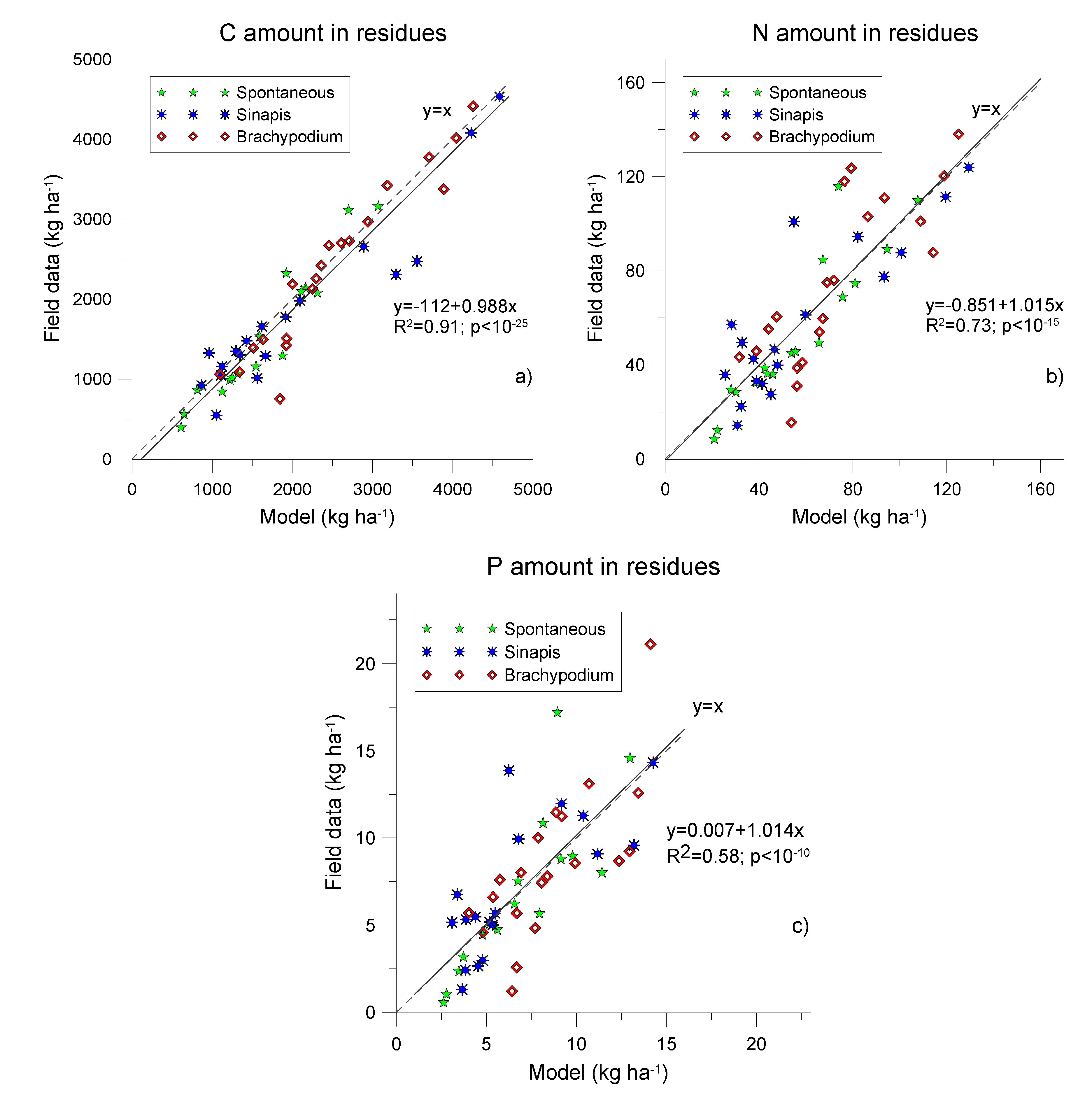
3.2. C, N and P Modelling

The relationship between residual C and aboveground residue amount is expressed in

Table 7. Linear relationship between residual C and aboveground residue amount.

Cover Crop	Parameter
	α	β
Brachypodium	−39.02	0.4128
Sinapis	−62.28	0.4238
Spontaneous	1.77	0.3948

Model: Residual C_i,t = α + β × Residue Amount_i,t + ε_i,t. The subscript i,t refers to sample i, measured in instant t. In all cases, R² > 0.99; p-value < 10⁻¹⁰.

. This relationship was used to predict the C amount in the residues since it showed a coefficient of determination close to one. In all cases, the parameter β, which was equal to the increment in C amount per unit of increment of residue amount, was very similar. The intercepts were also similar. This implies a very similar C concentration in these herbaceous residues (Table 4), as reported by Ma et al. [62].

The relationship between the N and P amount in the residues with respect to the residue amount (not shown) was also significant but with a higher scatter. For this reason, k_N and k_P were determined according to Equation (8). The k_N was equal to 0.00014 °C⁻¹ for Brachypodium, 0.00026 °C⁻¹ for Sinapis and 0.00021 °C⁻¹ for the controlled spontaneous vegetation. Similarly, the k_P value was equal to 0.00018 °C⁻¹ for Brachypodium, 0.00029 °C⁻¹ for Sinapis and 0.00033 °C⁻¹ for the controlled spontaneous vegetation. This result implies that the release rate was, on average, always higher for P than for N. This was previously observed in pea under no-till farming [43]. Wang et al. [29] indicated that P and K in straw are released during short-term straw return, while C and N are released during long-term straw return. In our case, only K was clearly released in the short term.

The abovementioned coefficients k_N and k_P determined the rate of release. The higher the coefficient, the faster the element was released. Thus, P release rates were always higher than N release rates: 29% higher for Brachypodium, 12% for Sinapis, and 57% for the controlled spontaneous vegetation.

The predictions of decomposition according to the Rickman model varied among the different elements studied. Figure 2, Figure 3 and Figure 4 show the experimental evolution of the C, N and P amounts in the aboveground residues throughout the four field campaigns. The figures also depict the results of the Rickman model with the corresponding adjusted k coefficient and its 95% confidence interval. Most experimental measurements were within the 95% confidence interval (Figure 2, Figure 3 and Figure 4), ranging from 65% to 88% for the studied CCs.

The best E values were always obtained for C in all the CCs, ranging from 0.64 to 0.72 (

Table 8. Coefficients for model evaluation and statistics obtained in simulations.

Species			Element
			C	N	P
Brachypodium distachyon	Coefficient	E	0.69	0.38	0.28
		CRM	−0.02	−0.12	−0.14
	Observed values (kg ha−1)	Mean	2433	76	8.8
		SD	1167	41	5.5
	Simulated values (kg ha−1)	Mean	2493	85	9.9
		SD	898	31	4.7
	Correlation	rxy ✡	0.84	0.67	0.62
Sinapis alba	Coefficient	E	0.64	0.54	0.37
		CRM	−0.12	0.08	0.08
	Observed values (kg ha−1)	Mean	1815	60	7.2
		SD	1155	40	5.1
	Simulated values (kg ha−1)	Mean	2039	55	6.7
		SD	1111	29	3.7
	Correlation	rxy ✡	0.83	0.75	0.63
Spontaneous soil cover	Coefficient	E	0.72	0.50	0.44
		CRM	−0.10	−0.04	−0.01
	Observed values (kg ha−1)	Mean	1503	54	6.8
		SD	900	39	5.1
	Simulated values (kg ha−1)	Mean	1647	57	6.7
		SD	716	31	4.6
	Correlation	rxy ✡	0.83	0.72	0.70

r_xy:: Pearson’s correlation coefficient. ^✡ In all cases, correlations were significant, with p < 10⁻¹⁰. E: coefficient of efficiency. CRM: coefficient of residual mass.

). Similarly, the worst E values per CC were obtained for P in all cases, with values ranging between 0.28 and 0.44. The same pattern was shown by the coefficient r_xy, as shown in Table 8. This result means that the C residue amount was the best fitted variable, while P presented the worst fit. We hypothesize that this scenario could have been partially attributable to easily leachable P compounds [69]. At a global level, there was a slight overestimation by the models, which was manifested in seven out of the nine negative values of the CRM coefficient.

Pearson’s linear correlation values between the observed and simulated values ranged between 0.62 and 0.84, with p < 10⁻⁵ in all cases (Table 8). The sequence of the values of this coefficient was always C > N > P. Regarding the coefficient of efficiency and following the criterion of Van Liew and Garbretch [60], the C, N and P amounts simulated by the Rickman model can be considered satisfactory (0.36 < E < 0.75) regardless of the CC, with the only exception being P in Brachypodium (E = 0.28).

Similarly, there was good agreement between the observed and simulated values in all CCs regarding the mean values (Table 8). The standard deviation of the observed values was always higher than that of the simulated values. This is logical since the models showed an expected value, i.e., a mean value. Nevertheless, the observed values exhibited great field variability.

This is a consequence of the short-distance natural variability in environmental variables [70,71], which is clearly evident when grab sampling is employed, as was the case here. However, grab sampling is a more realistic method than litterbags [33] since accessibility of the residues to decomposers can be limited by mesh openings. In addition, litterbags can alter the microclimate of the residues and put in contact with the soil some residues that would be standing for a long time period under natural conditions [36].

The Rickman model here exposed is an improvement of the Douglas–Rickman model, and has been extensively used with good results in a wide variety of climates and crops to predict decomposition or to aid in soil carbon modeling [41,43,45,72,73].

As seen in Figure 5a–c, the overall performance of the model applied to C, N and P is suitable. The slope is practically one in all cases, and the points are generally near the bisector, especially in the case of C (Figure 5a). In this element, the linear fit is always under the bisector, since the intercept was equal to −112 kg ha⁻¹. It is reflected in negative values of CRM (Table 8), ranging from −0.02 to −0.12. Likewise, the highest coefficient of determination was obtained for C in all CCs, thus reflecting the best adjustment, which agrees with the highest E and coefficient of correlation for this element in all CCs. Similarly, the behavior of the model for N and P is also in line with the results in Table 8, with P being the worst fitted element.

The 95% confidence interval of the slope contained one in C, N and P. Therefore, the use of the Rickman model to determine C amounts, as well as simple exponential models for N and P, have proven to be adequate to predict the average C, N and P remaining in the aboveground residues under Mediterranean conditions.

4. Conclusions

The studied CCs released a large amount of C along the decomposition cycle, ranging from 0.8 Mg ha⁻¹yr⁻¹ to 1.2 Mg ha⁻¹yr⁻¹ in the aboveground residues. The release of C, N and P accounted for 42 to 57% of the total amount at the beginning of the decomposition cycles. The percentage of K release was always noticeably higher than that of C, N and P, ranging from 80% to 90% of the total amount in the CC residues.

The lowest amount of C, N and P released from residues was obtained in the spontaneous CC. It was mainly because it yielded significantly less residue after harvest than the newly proposed CCs. The opposite result was obtained for K, as the spontaneous CC increased K release by 11% with respect to Brachypodium and 31% with respect to Sinapis. Overall, the newly proposed CCs seem to be more promising for providing C and N to the soil than the spontaneous CC, which is currently the most used CC by farmers.

Under realistic field conditions, the Rickman model and the exponential model showed a good performance to predict C, N and P release from aboveground residues, with P being the worst fitted element. These findings could help develop better practices under conservation agriculture and estimate nutrients release in olive groves.

References

1. FAO Agricultural Statistics. Available online: http://faostat.fao.org (accessed on 29 December 2019).
2. Mairech, H.; López-Bernal, Á.; Moriondo, M.; Dibari, C.; Regni, L.; Proietti, P.; Villalobos, F.J.; Testi, L. Is new olive farming sustainable? A spatial comparison of productive and environmental performances between traditional and new olive orchards with the model OliveCan. Agric. Syst. 2020, 181, 102816. [Google Scholar] [CrossRef]
3. MAPA. Encuesta Sobre Superficies Y Rendimientos de Cultivos (ESYRCE): Resultados 2019. 2019, p. 176. Available online: https://www.mapa.gob.es/es/estadistica/temas/estadisticas-agrarias/boletin2019_tcm30-536911.pdf (accessed on 27 May 2020).
4. Cerdà, A.; Lavee, H.; Romero-Díaz, A.; Hooke, J.; Montanarella, L. Soil erosion and degradation in Mediterranean-type ecosystems. Land Degrad. Dev. 2010, 21, 71–74. [Google Scholar] [CrossRef]
5. Espejo-Pérez, A.J.; Rodríguez-Lizana, A.; Ordóñez, R.; Giráldez, J.V. Soil loss and runoff reduction in olive-tree dry-farming with cover crops. Soil Sci. Soc. Am. J. 2013, 77, 2140–2148. [Google Scholar] [CrossRef] [Green Version]
6. Ordóñez-Fernández, R.; Rodríguez-Lizana, A.; Espejo-Pérez, A.J.; González-Fernández, P.; Saavedra, M.M. Soil and available phosphorus losses in ecological olive groves. Eur. J. Agron. 2007, 27, 144–153. [Google Scholar] [CrossRef]
7. Miranda-Fuentes, A.; Rodríguez-Lizana, A.; Gil, E.; Agüera-Vega, J.; Gil-Ribes, J.A. Influence of liquid-volume and airflow rates on spray application quality and homogeneity in super-intensive olive tree canopies. Sci. Total Environ. 2015, 537, 250–259. [Google Scholar] [CrossRef] [PubMed]
8. Parras-Alcántara, L.; Lozano-García, B.; Keesstra, S.; Cerdá, A.; Brevik, E.C. Long-term effects of soil management on ecosystem services and soil loss estimation in olive grove top soils. Sci. Total Environ. 2016, 571, 498–506. [Google Scholar] [CrossRef]
9. Lal, R. Restoring soil quality to mitigate soil degradation. Sustainability 2015, 7, 5875–5895. [Google Scholar] [CrossRef] [Green Version]
10. Kassam, A.; Friedrich, T.; Derpsch, R.; Lahmar, R.; Mrabet, R.; Basch, G.; González-Sánchez, E.J.; Serraj, R. Conservation agriculture in the dry Mediterranean climate. Field Crop. Res. 2012, 132, 7–17. [Google Scholar] [CrossRef] [Green Version]
11. Carbonell-Bojollo, R.; Ordóñez-Fernández, R.; Rodríguez-Lizana, A. Influence of olive mill waste application on the role of soil as a carbon source or sink. Clim. Chang. 2010, 102, 625–640. [Google Scholar] [CrossRef]
12. Rodríguez-Lizana, A.; Ordóñez, R.; Espejo-Pérez, A.J.; González, P. Plant cover and control of diffuse pollution from P in olive groves. Water Air Soil Pollut. 2007, 181, 17–34. [Google Scholar] [CrossRef]
13. Durán-Zuazo, V.H.; Rodríguez-Pleguezuelo, C.R. Soil-erosion and runoff prevention by plant covers. A review. Agron. Sustain. Dev. 2008, 28, 65–86. [Google Scholar] [CrossRef] [Green Version]
14. Keesstra, S.D.; Rodrigo-Comino, J.; Novara, A.; Giménez-Morera, A.; Pulido, M.; Di Prima, S.; Cerdà, A. Straw mulch as a sustainable solution to decrease runoff and erosion in glyphosate-treated clementine plantations in Eastern Spain. An assessment using rainfall simulation experiments. Catena 2019, 174, 95–103. [Google Scholar] [CrossRef]
15. Saavedra, M.; Pastor, M. Sistemas de Cultivo en Olivar: Manejo de Malas Hierbas y Herbicidas; Editorial Agrícola Española: Madrid, Spain, 2002. [Google Scholar]
16. MAGRAMA. Encuesta Sobre Superficies Y Rendimientos de Cultivo (ESYRCE): Análisis de las Técnicas de Mantenimiento de Los Suelos Y de Los Métodos de Siembra en España. 2019. Available online: https://www.mapa.gob.es/es/estadistica/temas/estadisticas-agrarias/cubiertas2019_tcm30-526244.pdf (accessed on 28 May 2020).
17. Repullo, M.A.; Carbonell, R.; Hidalgo, J.; Rodríguez-Lizana, A.; Ordóñez, R. Using olive pruning residues to cover soil and improve fertility. Soil Tillage Res. 2012, 124, 36–46. [Google Scholar] [CrossRef]
18. Rodríguez-Lizana, A.; Pereira, M.J.; Ribeiro, M.C.; Soares, A.; Márquez-García, F.; Ramos, A.; Gil-Ribes, J. Assessing local uncertainty of soil protection in an olive grove area with pruning residues cover: A geostatistical cosimulation approach. Land Degrad. Dev. 2017, 28, 2086–2097. [Google Scholar] [CrossRef]
19. Ordóñez-Fernández, R.; Repullo-Ruibérriz de Torres, M.A.; Román-Vázquez, J.; González-Fernández, P.; Carbonell-Bojollo, R. Macronutrients released during the decomposition of pruning residues used as plant cover and their effect on soil fertility. J. Agric. Sci. 2015, 153, 615–630. [Google Scholar] [CrossRef]
20. Rodríguez-Lizana, A.; Espejo-Pérez, A.J.; González-Fernández, P.; Ordóñez-Fernández, R. Pruning residues as an alternative to traditional tillage to reduce erosion and pollutant dispersion in olive groves. Water Air Soil Pollut. 2008, 193, 165–173. [Google Scholar] [CrossRef]
21. Tribouillois, H.; Cohan, J.P.; Justes, E. Cover crop mixtures including legume produce ecosystem services of nitrate capture and green manuring: Assessment combining experimentation and modelling. Plant Soil 2016, 401, 347–364. [Google Scholar] [CrossRef]
22. Alcántara, C.; Sánchez, S.; Pujadas, A.; Saavedra, M. Brassica species as winter cover crops in sustainable agricultural systems in southern spain. J. Sustain. Agric. 2009, 33, 619–635. [Google Scholar] [CrossRef]
23. García-Díaz, A.; Bienes, R.; Sastre, B.; Novara, A.; Gristina, L.; Cerdà, A. Nitrogen losses in vineyards under different types of soil groundcover. A field runoff simulator approach in central Spain. Agric. Ecosyst. Environ. 2017, 236, 256–267. [Google Scholar] [CrossRef]
24. Alcántara, C.; Pujadas, A.; Saavedra, M. Management of Sinapis alba subsp. mairei winter cover crop residues for summer weed control in southern Spain. Crop Prot. 2011, 30, 1239–1244. [Google Scholar] [CrossRef]
25. Jurado-Bello, J.; De Haro, A.; Hidalgo, J.; Hidalgo, J.C.; Vega, V.; Bejarano-Alcázar, J. Evaluación de la eficacia de enmiendas basadas en especies crucíferas implantadas como cubiertas vegetales para el control de la verticilosis del olivo en condiciones de campo. In Proceedings of the XVI Scientific-Technical Symposium of Olive Oil Expoliva, Jaén, Spain, 8–11 May 2013. [Google Scholar]
26. De Torres, M.A.R.R.; Ordóñez-Fernández, R.; Giráldez, J.V.; Márquez-García, J.; Laguna, A.; Carbonell-Bojollo, R. Efficiency of four different seeded plants and native vegetation as cover crops in the control of soil and carbon losses by water erosion in olive orchards. Land Degrad. Dev. 2018, 29, 2278–2290. [Google Scholar] [CrossRef]
27. Reicosky, D.C.; Archer, D.W. Moldboard plow tillage depth and short-term carbon dioxide release. Soil Tillage Res. 2007, 94, 109–121. [Google Scholar] [CrossRef]
28. Dong, S.; Ma, Z.; Wang, L.; Yan, C.; Liu, L.; Gong, Z.; Cui, G. Decomposition and nutrient release characteristics of incorporated soybean and maize straw in northeast China. Ekoloji 2019, 28, 2119–2129. [Google Scholar]
29. Wang, Y.; Adnan, A.; Wang, X.; Shi, Y.; Yang, S.; Ding, Q.; Sun, G. Nutrient recycling, wheat straw decomposition, and the potential effect of straw shear strength on soil mechanical properties. Agronomy 2020, 10, 314. [Google Scholar] [CrossRef] [Green Version]
30. Ramirez-Garcia, J.; Gabriel, J.L.; Alonso-Ayuso, M.; Quemada, M. Quantitative characterization of five cover crop species. J. Agric. Sci. 2015, 153, 1174–1185. [Google Scholar] [CrossRef] [Green Version]
31. Weinert, T.L.; Pan, W.L.; Moneymaker, M.R.; Santo, G.S.; Stevens, R.G. Nitrogen recycling by nonleguminous winter cover crops to reduce leaching in potato rotations. Agron. J. 2002, 94, 365–372. [Google Scholar] [CrossRef]
32. Gómez-Muñoz, B.; Hatch, D.J.; Bol, R.; García-Ruiz, R. Nutrient dynamics during decomposition of the residues from a sown legume or ruderal plant cover in an olive oil orchard. Agric. Ecosyst. Environ. 2014, 184, 115–123. [Google Scholar] [CrossRef]
33. Ruffo, M.L.; Bollero, G.A. Modeling rye and hairy vetch residue decomposition as a function of degree-days and decomposition-days. Agron. J. 2003, 95, 900–907. [Google Scholar] [CrossRef]
34. Tian, G.; Kang, B.; Brussaard, L. Biological effect of plant residues with contrasting chemical compositions under humid tropical conditions-decomposition and nutrient release. Soil Biol. Biochem. 1992, 24, 1051–1060. [Google Scholar] [CrossRef]
35. Ágoston-Szabó, E.; Schöll, K.; Kiss, A.; Dinka, M. Mesh size and site effects on leaf litter decomposition in a side arm of the River Danube on the Gemenc floodplain (Danube-Dráva National Park, Hungary). Hydrobiologia 2016, 774, 53–68. [Google Scholar] [CrossRef] [Green Version]
36. Bokhorst, S.; Wardle, D.A. Microclimate within litter bags of different mesh size: Implications for the “arthropod effect” on litter decomposition. Soil Biol. Biochem. 2013, 58, 147–152. [Google Scholar] [CrossRef]
37. Piccini, C.; Marchetti, A.; Francaviglia, R. Estimation of soil organic matter by geostatistical methods: Use of auxiliary information in agricultural and environmental assessment. Ecol. Indic. 2014, 36, 301–314. [Google Scholar] [CrossRef]
38. Wadoux, A.M.J.C.; Marchant, B.P.; Lark, R.M. Efficient sampling for geostatistical surveys. Eur. J. Soil Sci. 2019, 70, 975–989. [Google Scholar] [CrossRef]
39. Douglas, C.; Rickman, R. Estimating crop residue decomposition from air temperature, initial nitrogen content, and residue placement. Soil Sci. Soc. Am. J. 1992, 56, 272–278. [Google Scholar] [CrossRef]
40. Rickman, R.; Douglas, C.; Albrecht, S.; Berc, J. Tillage, crop rotation, and organic amendment effect on changes in soil organic matter. Environ. Pollut. 2002, 116, 405–411. [Google Scholar] [CrossRef]
41. Liang, Y.; Gollany, H.T.; Rickman, R.W.; Albrecht, S.L.; Follett, R.F.; Wilhelm, W.W.; Novak, J.M.; Douglas, C.L. Simulating soil organic matter with CQESTR (v. 2.0): Model description and validation against long-term experiments across North America. Ecol. Modell. 2009, 220, 568–581. [Google Scholar] [CrossRef]
42. Rodríguez-Lizana, A.; De Torres, M.A.R.R.; Carbonell-Bojollo, R.; Alcántara, C.; Ordóñez-Fernández, R. Brachypodium distachyon, Sinapis alba, and controlled spontaneous vegetation as groundcovers: Soil protection and modeling decomposition. Agric. Ecosyst. Environ. 2018, 265, 62–72. [Google Scholar] [CrossRef]
43. Rodríguez-Lizana, A.; Carbonell, R.; González, P.; Ordóñez, R. N, P and K released by the field decomposition of residues of a pea-wheat-sunflower rotation. Nutr. Cycl. Agroecosystems 2010, 87, 199–208. [Google Scholar] [CrossRef]
44. Laloy, E.; Bielders, C.L. Modelling intercrop management impact on runoff and erosion in a continuous maize cropping system: Part I. model description, global sensitivity analysis and bayesian estimation of parameter identifiability. Eur. J. Soil Sci. 2009, 60, 1005–1021. [Google Scholar] [CrossRef]
45. Gollany, H.T.; Nash, P.R.; Johnson, J.M.F.; Barbour, N.W. Predicted annual biomass input to maintain soil organic carbon under contrasting management. Agron. J. 2019, 111, 11. [Google Scholar] [CrossRef]
46. Gollany, H.T.; Elnaggar, A.A. Simulating soil organic carbon changes across toposequences under dryland agriculture using CQESTR. Ecol. Modell. 2017, 355, 97–104. [Google Scholar] [CrossRef] [Green Version]
47. Quebrajo, L.; Pérez-Ruiz, M.; Rodríguez-Lizana, A.; Agüera, J. An approach to precise nitrogen management using hand-held crop sensor measurements and winter wheat yield mapping in a mediterranean environment. Sensors 2015, 15, 5504–5517. [Google Scholar] [CrossRef] [PubMed] [Green Version]
48. Soil Survey Staff. Keys to Soil Taxonomy, 12th ed.; USDA-Natural Resources Conservation Service: WAshington, DC, USA, 2014. [Google Scholar]
49. Chochois, V.; Voge, J.P.; Rebetzke, G.J.; Watt, M. Variation in adult plant phenotypes and partitioning among seed and stem-borne roots across Brachypodium distachyon accessions to exploit in breeding cereals for well-watered and drought environments. Plant Physiol. 2015, 168, 953–967. [Google Scholar] [CrossRef] [PubMed] [Green Version]
50. Hajzler, M.; Klimesová, J.; Streda, T.; Vejrazka, K.; Marcek, V.; Cholastová, T. Root system production and aboveground biomass production of chosen cover crops. Eng. Technol. 2012, 69, 713–718. [Google Scholar]
51. Lohmann, M.; Scheu, S.; Müller, C. Decomposers and root feeders interactively affect plant defence in Sinapis alba. Oecologia 2009, 160, 289–298. [Google Scholar] [CrossRef] [PubMed] [Green Version]
52. De la Peña, M.; González-Moro, M.B.; Marino, D. Providing carbon skeletons to sustain amide synthesis in roots underlines the suitability of Brachypodium distachyon for the study of ammonium stress in cereals. AoB Plants 2019, 11, 1–11. [Google Scholar] [CrossRef] [PubMed]
53. Goldberg, K.; Iglewicz, B. Bivariate extensions of the boxplot. Technometrics 1992, 34, 307–320. [Google Scholar] [CrossRef]
54. Wilcox, R. Introduction to Robust Estimation and Hypothesis Testing, 2nd ed.; Elsevier Academic Press: Burlington, CO, USA, 2010; ISBN 0-12-751542-9. [Google Scholar]
55. Giloni, A.; Padberg, M. Least trimmed squares regression, least median squares regression, and mathematical programming. Math. Comput. Model. 2002, 35, 1043–1060. [Google Scholar] [CrossRef]
56. Klemes, V. Operational testing of hydrological simulation models. Hydrol. Sci. J. 1986, 31, 13–24. [Google Scholar] [CrossRef]
57. Zema, D.A.; Bingner, R.; Denisi, P.; Govers, G.; Licciardello, F.; Zimbone, S.M. Evaluation of runoff, peak flow and sediment yield events simulated by annagnps in a belgian agricultural watershed. Land Degrad. Dev. 2012, 23, 205–215. [Google Scholar] [CrossRef]
58. Nash, J.; Sutcliffe, J. River flow forecasting through conceptual models: Part I. A discussion of principles. J. Hidrol. 1970, 10, 282–290. [Google Scholar] [CrossRef]
59. Loague, K.; Green, R.E. Statistical and graphical methods for evaluating solute transport models: Overview and application. J. Contam. Hidrol. 1991, 7, 51–73. [Google Scholar] [CrossRef]
60. Van Liew, M.W.; Garbretch, J. Hydrologic simulation of the Little Washita River experimental watersed using SWAT. J. Am. Water Resour. Assoc. 2003, 39, 413–426. [Google Scholar] [CrossRef]
61. R Core Team. R: A Language and Environment for Statistical Computing; R Foundation for Statistical Computing: Vienna, Austria, 2019; Available online: https://www.R-project.org (accessed on 17 July 2020).
62. Ma, S.; He, F.; Tian, D.; Zou, D.; Yan, Z.; Yang, Y.; Zhou, T.; Huang, K.; Shen, H.; Fang, J. Variations and determinants of carbon content in plants: A global synthesis. Biogeosciences 2018, 15, 693–702. [Google Scholar] [CrossRef] [Green Version]
63. Pimentel, L.G.; Cherubin, M.R.; Oliveira, D.M.S.; Cerri, C.E.P.; Cerri, C.C. Decomposition of sugarcane straw: Basis for management decisions for bioenergy production. Biomass Bioenergy 2019, 122, 133–144. [Google Scholar] [CrossRef]
64. Zhang, P.; Chen, X.; Wei, T.; Yang, Z.; Jia, Z.; Yang, B.; Han, Q.; Ren, X. Effects of straw incorporation on the soil nutrient contents, enzyme activities, and crop yield in a semiarid region of china. Soil Tillage Res. 2016, 160, 65–72. [Google Scholar] [CrossRef]
65. Sui, N.; Zhou, Z.; Yu, C.; Liu, R.; Yang, C.; Zhang, F.; Song, G.; Meng, Y. Yield and potassium use efficiency of cotton with wheat straw incorporation and potassium fertilization on soils with various conditions in the wheat- cotton rotation system. Field Crop. Res. 2015, 172, 132–144. [Google Scholar] [CrossRef]
66. Aznar-Sánchez, J.A.; Velasco-Muñoz, J.F.; López-Felices, B.; Del Moral-Torres, F. Barriers and Facilitators for Adopting Sustainable Soil Management Practices in Mediterranean Olive Groves. Agronomy 2020, 10, 506. [Google Scholar] [CrossRef] [Green Version]
67. Li, J.; Lu, J.; Li, X.; Ren, T.; Cong, R.; Zhou, L. Dynamics of potassium release and adsorption on rice straw residue. PLoS ONE 2014, 9, e90440. [Google Scholar] [CrossRef]
68. Ordóñez-Fernández, R.; De Torres, M.A.R.R.; Márquez-García, J.; Moreno-García, M.; Carbonell-Bojollo, R.M. Legumes used as cover crops to reduce fertilisation problems improving soil nitrate in an organic orchard. Eur. J. Agron. 2018, 95, 1–13. [Google Scholar] [CrossRef]
69. Wang, X.; Yang, H.; Liu, J.; Wu, J.; Chen, W.; Wu, J.; Zhu, L.; Bian, X. Effects of ditch-buried straw return on soil organic carbon and rice yields in a rice-wheat rotation system. Catena 2015, 127, 56–63. [Google Scholar] [CrossRef]
70. Goovaerts, P. Geostatistical modelling of uncertainty in soil science. Geoderma 2001, 103, 3–26. [Google Scholar] [CrossRef]
71. Keskin, H.; Grunwald, S. Regression kriging as a workhorse in the digital soil mapper’s toolbox. Geoderma 2018, 326, 22–41. [Google Scholar] [CrossRef]
72. Cavigelli, M.A.; Nash, P.R.; Gollany, H.T.; Rasmann, C.; Polumsky, R.W.; Le, A.N.; Conklin, A.E. Simulated soil organic carbon changes in maryland are affected by tillage, climate change, and crop yield. J. Environ. Qual. 2018, 47, 588–595. [Google Scholar] [CrossRef] [PubMed] [Green Version]
73. Ordóñez-Fernández, R.; Rodríguez-Lizana, A.; Carbonell, R.; González, P.; Perea, F. Dynamics of residue decomposition in the field in a dryland rotation under Mediterranean climate conditions in southern Spain. Nutr. Cycl. Agroecosystems 2007, 79, 243–253. [Google Scholar] [CrossRef]
Figure 1. Monthly rainfall and monthly average temperature in the research area from May 2008 to September 2011.
Agronomy 10 01041 g001
Figure 2. Measured and modelled C amounts in aboveground residues during the four decomposition cycles for spontaneous cover (a), Brachypodium (b) and Sinapis (c). The dashed lines represent estimations from the Rickman model [40].
Agronomy 10 01041 g002
Figure 3. Measured and modelled N amounts during the four decomposition cycles for spontaneous cover (a), Brachypodium (b) and Sinapis (c).
Agronomy 10 01041 g003
Figure 4. Measured and modelled P amounts during the four decomposition cycles for spontaneous cover (a), Brachypodium (b) and Sinapis (c).
Agronomy 10 01041 g004aAgronomy 10 01041 g004b
Figure 5. Measured versus estimated C (a), N (b) and P (c) amounts in the aboveground residues for the three types of cover crops and 4-year field trial. The dashed line is 1:1, and the straight line is the regression line.
Agronomy 10 01041 g005