Identifying Cotton Fields from Remote Sensing Images Using Multiple Deep Learning Networks

Abstract

Remote sensing imageries processed through empirical and deterministic approaches help predict multiple agronomic traits throughout the growing season. Accurate identification of cotton crop from remotely sensed imageries is a significant task in precision agriculture. This study aims to utilize a deep learning-based framework for cotton crop field identification with Gaofen-1 (GF-1) high-resolution (16 m) imageries in Wei-Ku region, China. An optimized model for the pixel-wise multidimensional densely connected convolutional neural network (DenseNet) was used. Four widely-used classic convolutional neural networks (CNNs), including ResNet, VGG, SegNet, and DeepLab v3+, were also used for accuracy assessment. The results infer that DenseNet can identify cotton crop features within a relatively shorter time about 5 h for training convergence. The model performance was examined by multiple indicators (P, F1, R, and mIou) produced through the confusion matrix, and the derived cotton fields were then visualized. The DenseNet model has illustrated considerable improvements in comparison with the preceding mainstream models. The results showed that the retrieval precision was 0.948, F1 score was 0.953, and mIou was 0.911. Furthermore, its performance is relatively better in discriminating cotton crop fields’ fine structures when clouds, mountain shadows, and urban built up.

1. Introduction

Cotton (Gossypium hirsutum L.) is an important economic crop in China. Xinjiang is the largest cotton producer in China, occupying an important income source both domestically and internationally. According to the statistical data from 2018 [1], the total cotton crop area of Wei-ku oasis, among the largest cotton crop belts in Xinjiang, was roughly ~312,760 hectares, 8.56% of the cotton area in Xinjiang. In the same (2018) fiscal year, the cotton production was ~626,316 tons, substantially contributing to the local GDP. Recently, due to an exponential increase in the cotton products demand, the cotton cropped area in Xinjiang has reached up to ~2.5 million hectares during the fiscal year 2019–2020 with a 78% production of the national level [2]. The warming trend and changing climate have threatened cotton productivity, especially due to water and energy cycle changes. Recent studies indicated that air humidity changes, precipitation, temperature, and sunshine duration collectively affect biological and cotton stalk productivity [3,4]. Traditionally, the statistical information is usually released through the end of the fiscal year that provides cumulative descriptive information of the area cropped, production, losses due to natural hazards, and many more. For a better prediction and forecast of the production, a continuous seasonal real-time cost-effective, and less laborious monitoring is an important challenge [5,6].

Remote sensing techniques have the advantages of monitoring agricultural practices from multiple viewpoints such as crop growth monitoring [7], disease identification [8], yield forecast [9], crop area estimation [10], weed identification [11], and crop water requirement estimations [12]. At present, the remote sensing identification of crop extent area is mainly estimated through supervised classification that relies on a substantial amount of training data [13]. Many algorithms for crop area extraction from satellite images have been proposed, including spectral analysis classification [14,15] and machine learning [16,17,18,19]. Chen, S. et al. [16] used 250 m resolution MODIS-NDVI data and spectral analysis for cropland distribution patterns in Northeast China. The results inferred that the proposed approach is suitable for multiple crop classification under limited experimental conditions and single large crop cultivated areas. Mathur, A. [17] demonstrated that using a support vector machine (SVM) adds to agriculture classification under limited support vectors and highlighted the possibility of further reduction in training set without losing classification accuracy. Ishak, A. J. [19] employed a decision tree for weed classification, based on achieved accuracy rate and selection of optimal feature vectors, the CART algorithm performed well in weed recognition.

For crop feature identification and mapping, the remote sensing imageries are obtained either through airborne satellites [20], unmanned air vehicles (UAV’s) [21], or unmanned ground vehicles (UGV’s) [22]. These images are then processed with machine learning and deep learning techniques for achieving the required crop feature mapping and identification in time and space dimensions. Satellite data are generally used in large-scale monitoring, while UAV and UGV are used for small-scale monitoring [23]. On a much local and small scale, the cotton crop identification and mapping from remotely sensed imageries with a larger swath width is challenging. Although Gong Peng’s team publicly shared a 10-m resolution global land cover type product [24], among other constraints, the cotton crop as a land-cover class is limited and least explored in the existing data sets of land cover types shared globally. However, the study of an all-season sample database for improving Africa’s land-cover mapping with two classification schemes provides a reference for its application in mapping the cotton crop area, with less than 1% accuracy loss [25]. A similar approach will help in efficient and timely prediction of cotton acreage cultivated in remote areas, production estimation, crop area loss due to natural hazards, and other relevant statistics cost-effectively and less laboriously. This can be an alternative to traditional methods that rely on sufficient prior knowledge, processing big data, and reducing computer hardware burden.

In recent years, deep learning techniques have been widely applied in earth sciences, especially in land cover classification and object identification [26]. Deep learning in remote sensing is eminent because of its ability to explicitly differentiate raw images’ spectral and spatial characteristics. Image texture reflects the brightness nature of the image and its spatial arrangement of the color [27]. Compared to the traditional methods, deep learning is characterized by adapting to a large sample size without predefining the rules for specific tasks [28]. As deep learning has been successfully applied in various domains, it’s precision agriculture application is relatively recent [29]. Andreas Kamilaris et al. [30] performed a survey of 40 research efforts that employed deep learning techniques applied to various agricultural challenge. They examined the particular agricultural problems under study and compared deep learning with other existing popular techniques regarding differences in classification or regression performance. The findings indicate that deep learning provides high accuracy, outperforming existing commonly used image processing techniques [30].

The convolutional neural network (CNN) is one of the most successful deep learning frameworks; it greatly reduces the training parameters [31], improving both the computing efficiency and generalization capability. Especially, CNN’s enhance image recognition ability through local connection and weight sharing [32]. CNN’s have been largely used for target detection and classification from an image, and many model structures have been put forward, such as the VGG [33], the ResNet [34], and the DenseNet structures [35].

Recently, multiple attempts with CNN structures have been made to innovate algorithms for identifying different types of targets in satellite and aerial images. Widely used images are from Landsat with 30 m spatial and 16 days temporal resolution [36]. China launched the Gaofen-1 (GF1) satellite in 2013, which is equipped with two full-color cameras with a resolution of 2 m, and a multispectral camera with a resolution of 16 m. The revisit period of the GF-1 satellite is about four days; it has self-evident advantages considering its spatio-temporal resolutions. GF-1 is a high-resolution remote sensing image containing richer spatial information than medium-resolution remote sensing images. According to this feature, we can extract more detailed field crop feature information for precision agriculture. Very few studies (as of now) has employed GF-1 satellite images for cropland extraction, particularly with the advanced state of the art deep learning techniques.

The purpose of this study is to use the GF-1 satellite images to identify the cotton crop using an improved DenseNet structure and describe the distribution of cotton field in this region, then applied it to cotton field area monitoring. This study’s main contributions are as follows: first, the sample cotton field data set in Wei-ku oasis is developed, followed by the improved DenseNet model application for cotton field identification. The rest of the paper is structured as Section 2 is study area and data; Section 3 is materials and methods; Section 4 is results, and Section 5 is discussion and conclusions.

2. Study Area and Data

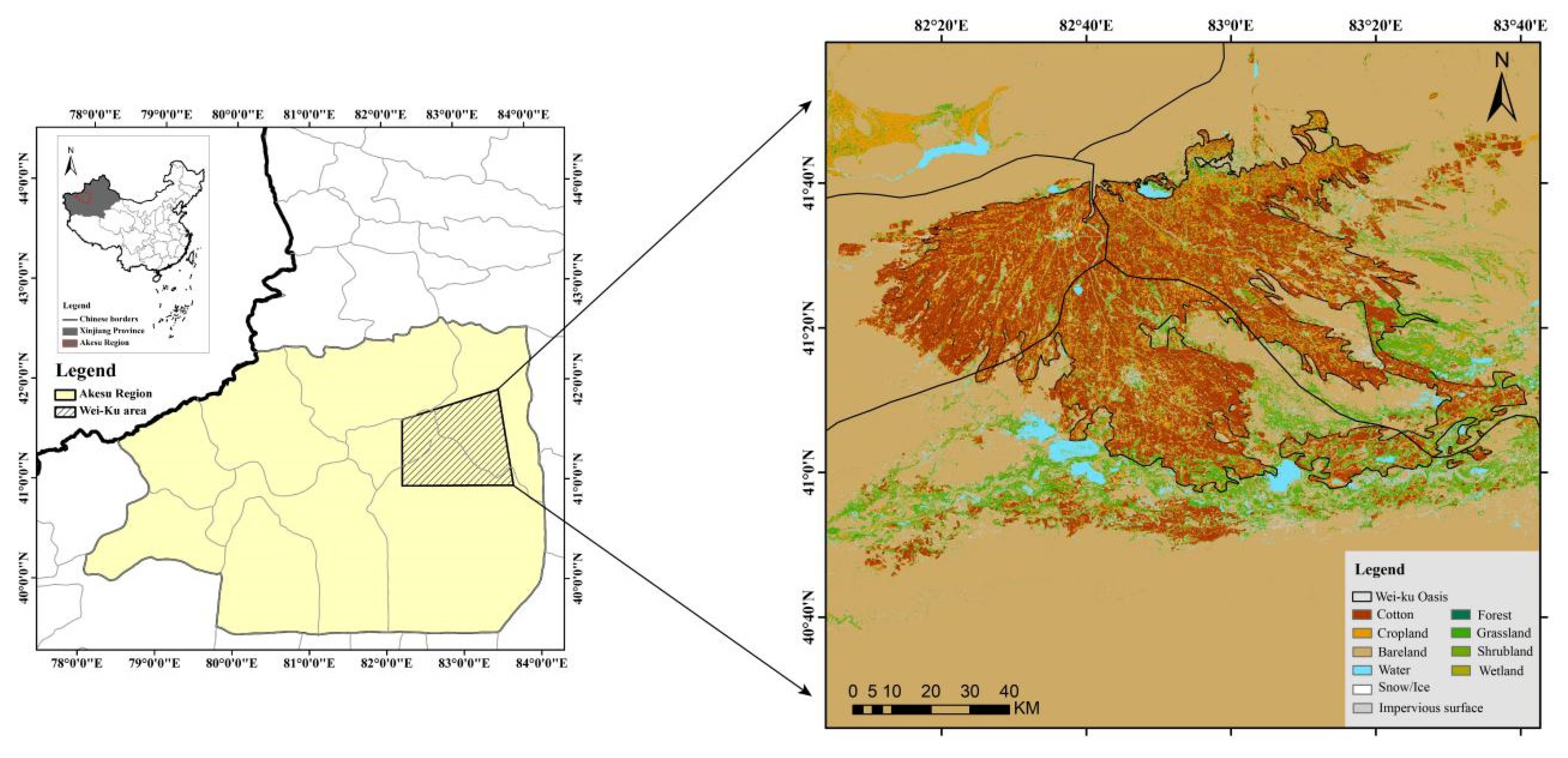
2.1. Study Area

The Wei-Ku Oasis (41°01′ N–41°43′ N and 82°09′ E–83°25′ E) is located (Figure 1) in the middle part of the Xinjiang Uygur Autonomous Region (Figure 1). Geographically, the Wei-Ku Oasis comprises three counties, namely Kuche, Xinhe, and Shaya, in the Akesu region. It has a temperate continental climate with limited precipitation of 51.6 mm annually and a mean temperature of 11.5 °C [37]. The annual average daily sunshine hours are ~13 h, and the diurnal temperature variation is higher between day and night, which is very suitable for cotton crop cultivation. The Wei-Ku Oasis is one of the major cotton-producing regions in the country, accounting for more than one-third of China’s cotton production. Cotton is planted in April and harvested from late September to early October.

2.2. Data

The GF-1 satellite images during September from 2016 to 2018 are used to monitor the cotton crop area; due to cotton crop phenology, September is relatively the best time to monitor the cropped area. The GF-1 satellite carries a wide-field of view (WFV) camera with a spectral range of 450–890 nm, and the multispectral channels are blue (450–520 nm), green (520–590 nm), red (630–690 nm), and near-infrared band (770–890 nm) respectively. The GF-1 satellite has a swath width of 800 km and a revisit period of 4 days, and the WFV camera has a spatial resolution of 16 m. In brief, it has a relatively short revisit time, high spatial resolution, and wide swath, providing state-of-the-art data for agriculture application. The images are available from China Resources Satellite Application Center (http://www.cresda.com/CN/). Blue, green, red, and near-infrared bands from the WFV camera are used as inputs of the current study’s CNN models.

2.3. Data Pre-Processing

The image preprocessing includes five steps; first, the images were enhanced to eliminate shadow and variable illumination [38]. Second, RPC Orthorectification, a type of geometric orthotropic correction used in remote sensing image data, was applied to the images. Then, the ground truth for cotton was labeled using several irregular shape annotations on pixel-level as training samples. After that, all the images were resized to the uniform size of 224 × 224 pixels to improve the model training efficiency. The initial number of these samples is 5500. Finally, data-augmentation techniques were used to enlarge the number of training samples to 16,500 artificially.

Data augmentation is a common way to expand training data variability by artificially enlarging a dataset via label-preserving transformations [39]. Typical augmentation techniques include left-right flipping, image re-scaling, and changing image color. In this study, we use horizontal and vertical flips to augment the samples. Training samples are created from the multispectral images in September from 2016 to 2018, and cotton identification experiments were performed in 2018.

3. Materials and Methods

3.1. CNN Models

3.1.1. VGG and ResNet

The VGG technique emerged in 2014 as a prominent deep CNN [31] and has been widely used as the backbone framework in numerous feature recognition tasks [40,41,42,43,44,45,46,47,48,49,50,51,52,53]. Studies on network depth and performance of the VGG structure have indicated that its depth affects the model’s performance to a certain extent [33]. The VGG network structure is very regular; several convolutional layers are followed by a pooling layer that reduces the image’s height and width. There is certain regularity in filter numbers in the convolutional layer, which doubles from 64 to 128 and then to 256 and 512. In this study, we use the VGG-19, which contains 19 convolutional and fully connected layers.

The VGG problem initially inspired the ResNet structure: the problem of degradation with continuously increasing network depths. The ResNet is a modified version of VGG, provided with 50 or 101 layers in common. Using a residual block that transmits information from input to the output directly, the degradation problem is solved, although the numbered layers are largely increased. In practice, the residual block is a combination of 1 × 1, 3 × 3, and 1 × 1 convolutional layers. The middle 3 × 3 convolutional layer first reduces the calculation under a dimension reduction 1 × 1 convolutional layer. It then restores it under another 1 × 1 convolutional layer, which maintains the accuracy and reduces the calculation amount. The layers may differ for ResNet, and we use ResNet-101 as a backbone in this study.

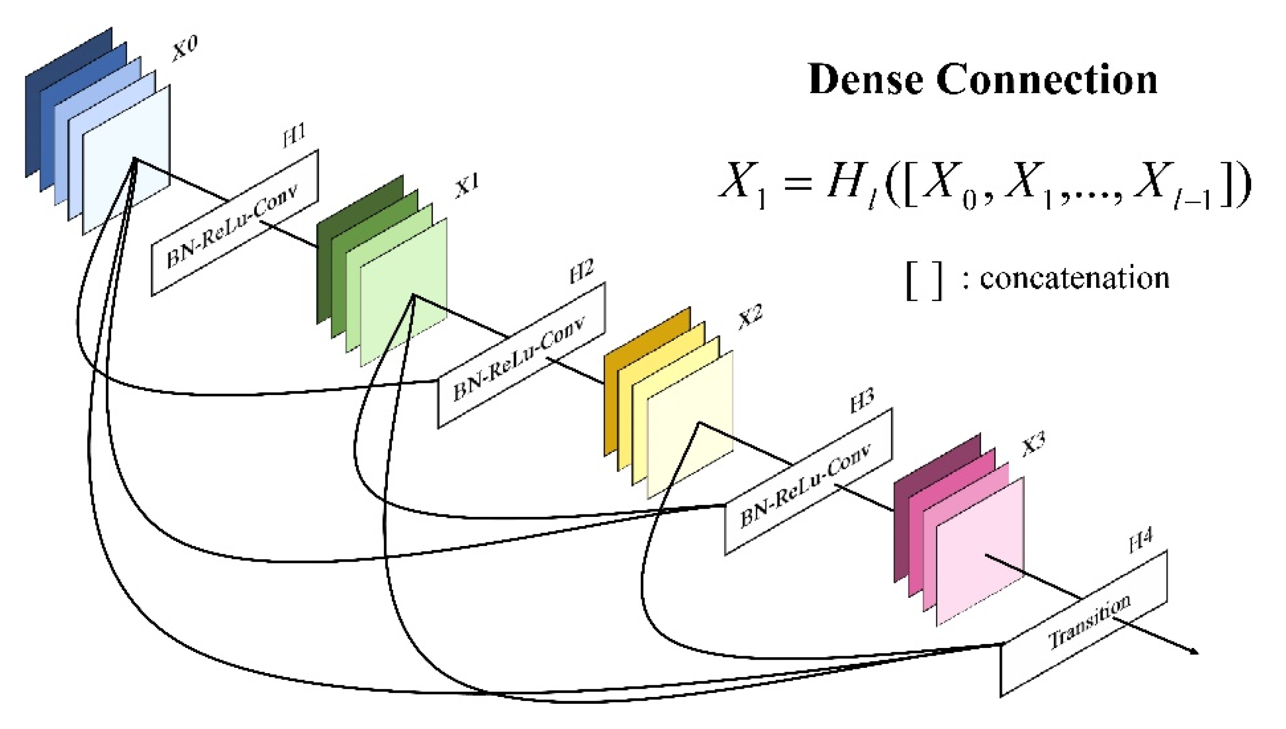
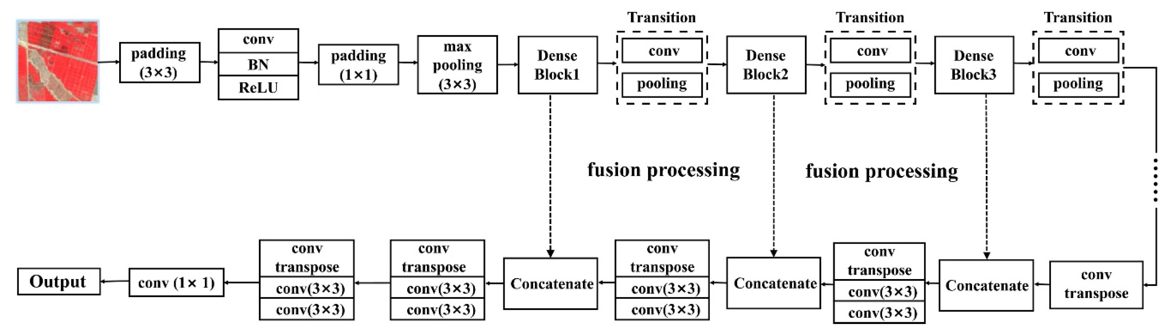
3.1.2. DenseNet and Improvement

The ResNet structure gets complicated when training a large number of model parameters. Its essential limitation lies in each convolutional layer being only able to obtain features from the front layers, making the best use of low-level convolutional features, leading to high-level convolutions’ information redundancy. The DenseNet structure was proposed to solve this problem, improving the network depth through dense connections of convolutional layers. It can also enhance the information flow and reduce gradients of the entire network, making them easy to train. Moreover, the dense connections have a regularization function, reducing overfitting when fewer training samples are involved. For DenseNet, the dense block is the most important architecture, as shown in Figure 2; it contains many layers connected by a dense connectivity pattern. There are direct connections from any layer to all subsequent layers, and the arbitrary current layer can receive the outputs of all preceding layers at its input [35].

Each dense block contains three compositions of batch normalization (BN) layers, rectified linear unit (ReLu) layers, and Convolutional (Conv) layers, aiming at linking the blocks to fuse different features. Unlike ResNet, this architecture does not only stack the features simply before passing them to the next layer but aggregates them in the concatenation process to realize characteristics and maximize reuse. Regarding a DenseNet model, the l layer’s input is the concatenation of the feature map from l to l-1 layer, and a nonlinear transformation is implemented subsequently. The dense connection of DenseNet fully utilizes features, making it directly accept the supervision of final loss to achieve deep supervision and resolve gradients disappearing.

This study uses an improved DenseNet structure (Figure 3) by Wang et al. [53] for cotton crop identification in the Wei-Ku Oasis. In the improved DenseNet, each dense block contains a 1 × 1 convolution and a 3 × 3 convolution operation; each transition block contains a 1 × 1 convolution and a 2 × 2 pooling operation. The operation of 1 × 1 convolution is used to reduce dimension and fuse the features from each channel. There are no dense connections between the dense block and the transition block. Specifically, an upsampling operation was executed in the improved DenseNet via transpose convolution to restore the spatial input information. The feature map from upsampling was concatenated to the feature map from the dense block in the down-sampling progress. The batch normalization (BN) and the rectified linear unit (ReLu) operation were carried out on the convolution layers.

3.1.3. SegNet and DeepLab v3+

SegNet and DeepLab v3+ are fully convolutional networks (FCNs) [54,55]. The FCNs, based on traditional CNN, convert the last fully connected layer and softmax output into a convolutional layer to achieve the pixel-level classification of images, which is the initial of image segmentation at semantic level [56,57,58,59]. Unlike traditional networks, the deconvolution structure is used to restore the resized feature map to its original size following feature recognition. This means that while maintaining the spatial input information acquired, the output with the same input size is acquired in degrees to get the target classification on a pixel level. Regardless of input size received, the networks are capable of training successfully. Following FCN, the SegNet [54] represents encoder-decoder structure, with the frontal 13 layers of VGG acting as the encoders and the max-pooling as the decoders to improve the segmentation resolution and increase the training accuracy. Proposed in 2018, the DeepLab v3+ is the latest development of the DeepLab series [59], which utilizes the deep CNNs involving atrous convolution in the decoder part, and the Astrous Spatial Pyramid Pooling (ASPP) is applied to collect multiple-scale information. Compared with its previous versions, DeepLab v3+ takes advantage of the decoder structure so that the lower-level characteristics and the higher-level ones can be stimulated to integrate further, improving the edge recognition and separation precision.

3.2. Experimental Setup

This study created 16,500 labeled samples with a suitable size of 224 × 224 × 4 from twelve GF-1 multispectral images in September 2016–2018, then used for network training and testing. Out of these samples, 13,200 images (80%) were randomly selected for training, and the remaining 3300 images (20%) were used for testing. To prevent overfitting due to the limited data samples and improve the model’s generalization, dropout was used for each epoch. The Adam optimization algorithm [57] was used to optimize the weight during the training process, and hyperparameters α1 = 0.900 and α2 = 0.999 are selected as recommended by the algorithm. Through several trials, the model was trained at the initial learning rate of λ = 10⁻⁴; it decreased by ten times every 30 epochs, which was considered the best. Besides, we set the batch size of 4, the growth rate as 32, the weight decay as 10⁻⁴, and the Nesterov momentum of 0.9 before training. Binary cross entropy was selected as a loss function, which was commonly used for binary segmentation. All the experiments were implemented based on the TensorFlow environment and executed on a Linux system with a GPU, NVIDIA 9.0, and 128 GB memory. All of these configured parameters were applied to the five models mentioned above.

3.3. Performance Evaluation

We introduced precision (P), recall (R), F-measure (Fα), and mean intersection over union (mIoU) to make a quantitative evaluation of different CNN networks based on the confusion matrix. Precision reflects the model accuracy, and recall represents the completeness of the captured cotton. In practice, precision and recall are contradictory to each other. When precision is high, recall is low. Furthermore, F1 (α = 1) is proposed to balance P, and R. Higher F1 indicates better identification result. The formulas for these evaluation indicators are [60]

$$P=\frac{TP}{TP+FP}$$

(1)

$$R=\frac{TP}{TP+FN}$$

(2)

$$F\alpha =\frac{(1+{\alpha }^2)\times P\times R}{{\alpha }^2(P+R)}$$

(3)

$$F1=\frac{2\times P\times R}{P+R}$$

(4)

All of these can be calculated from the true positives (TP), the true negatives (TN), the false positives (FP), and the false negatives (FN). The true positive (TP) represents the correct classification of a pixel as cotton, false positive (FP) represents the incorrect classification of a background pixel as cotton, and multiple detections of the same cotton. False-negative (FN) indicates an incorrect classification of cotton as a background pixel. As a result, precision gives insight into the amount of identified cotton, which was indeed cotton. Recall provides insight into the performance in capturing all true positives, thereby measuring how many of the cotton pixels were correctly identified and disregarding the number of false positives. To find the optimum balance between the two, the F1 score [60] is calculated as the harmonic mean between precision and recall. The mean intersection over union (mIoU) was used to evaluate the validation dataset’s processing precision. It generates two boxes called “predicted bounding box” and “ground-truth bounding box” and then compares the overlap rate between them. The formula of the mIoU is

$$mIoU=\frac{TP}{TP+FP+FN}$$

(5)

4. Results

Given the outstanding performance on water recognition by using the DenseNet recently, we consider to apply this improved DenseNet structure on cotton field identification and compare the results with other models to see its performance at identifying the cotton field. We have first made DenseNet pre-training with different types, ensuring that the DenseNet layer is optimal for cotton identification. Then, we compare its performance with the other models of ResNet, VGG, SegNet, and DeepLab v3+, considering the training efficiency and cotton identification accuracy.

4.1. Optimal DenseNet Layers

Most studies have shown that ResNet-101 has the best effect in surface feature classification tasks [61], compared with other layers. However, there are optimal layers for the DenseNet structure regarding specific tasks, and Huang [52] has proposed three kinds of layers, i.e., DenseNet129, DenseNet169, and DenseNet201. To define the optimal DenseNet layers for identifying cotton fields, we have conducted several experiments on the dense blocks with various layers and different parameter combinations. We have first halved the first convolution layers of three dense blocks from DenseNet121 and maintained the fourth block, which turned into DenseNet79. Next, we have attempted to halve the convolutional layers of four blocks, turning them into DenseNet63. Experiments are then implemented to train the five DenseNet models to find the optimal layers for our study.

Table 1. Evaluation matrices of different DenseNet models; P refers to precision, R refers to recall, F1 refers to F1 score, and mIoU refers to mean intersection over union. The optimal value for each metric is shown boldened.

Network	Time	P	R	F1	mIoU
DenseNet63	10,504 s	0.943	0.964	0.952	0.910
DenseNet79	18,824 s	0.948	0.960	0.953	0.911
DenseNet121	20,365 s	0.941	0.964	0.952	0.909
DenseNet169	23,602 s	0.940	0.966	0.953	0.910
DenseNet201	26,760 s	0.946	0.960	0.953	0.910

illustrates the performance of five DenseNet models, where the optimal values are shown in bold. It can be observed that with the increase of network layers, the training time increases subsequently. However, the performance fails to get better as layers growing, which means a relatively shallow model may be superior to deep ones in the DenseNet architecture for cotton crop identification. This is possibly due to the number limitation of the input samples; the features of cotton fields might as well be more easily identified, making excessive layers redundant. In brief, the DenseNet79 model appears to have the optimal performance regarding precision, F1 score, and mIoU indicators. Although its recall is lower than DenseNet169, the training time is largely reduced. Thence, DenseNet79 is the most suitable model to identify cotton fields in this study.

4.2. Training Efficiencies

Figure 4 illustrates the training losses of DenseNet, ResNet, VGG, SegNet, and DeepLab v3+ models, derived from the same set of samples. In the CNN, the loss function is calculated to measure the divergence between the input ground truth and the output result to optimize the model by continuously tuning weights. If we get a lower loss, the model is indicated to be more robust. The DenseNet appears to reach divergence rapidly with the lowest loss; the SegNet is second only to the DenseNet, followed by the DeepLab v3+ and the VGG, whereas the ResNet gets the highest loss. The training time of the five models is summarized in

Table 2. Training time of the DenseNet, ResNet, VGG, SegNet and DeepLab v3+ models.

Network	Time
DenseNet	18,824 s
ResNet	18,918 s
VGG	21,973 s
SegNet	25,000 s
DeepLab v3+	11,627 s

. The SegNet takes the longest time to train the model, which is more than six hours in our case.

Meanwhile, the DeepLab v3+ uses the shortest training time of fewer than four hours, indicating that the DeepLab v3+ is the easiest to train and computationally the cheapest to use. Although the DenseNet training time is not the shortest, it is second to the DeepLab v3+ and shorter than the VGG and the ResNet models. The training efficiency of DeepLab v3+ surpasses the DenseNet, because the backbone structure, MobileNet, is a lightweight network using the depth-wise separable convolution to reduce the amount of parameter and the calculation frequency [62].

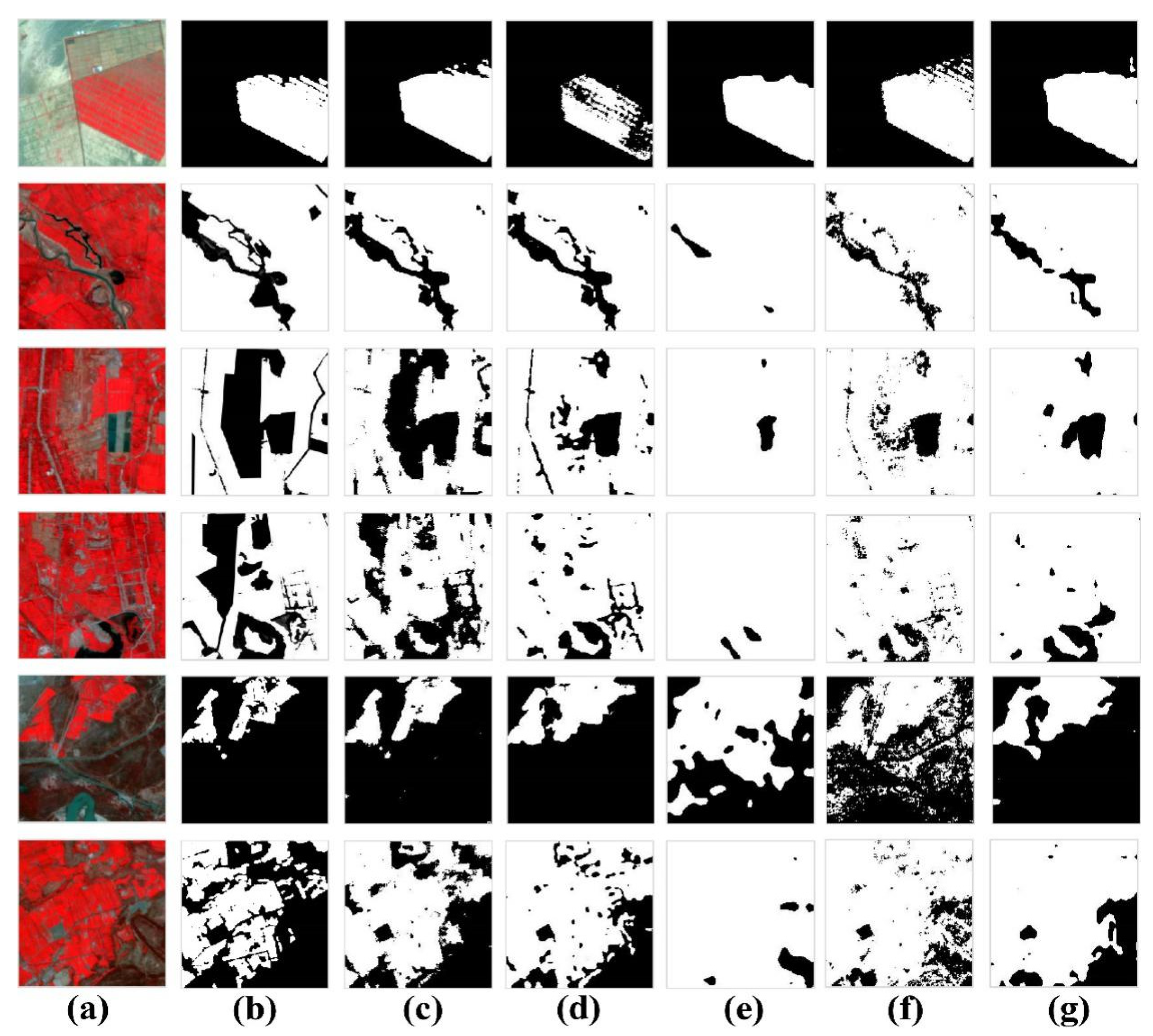
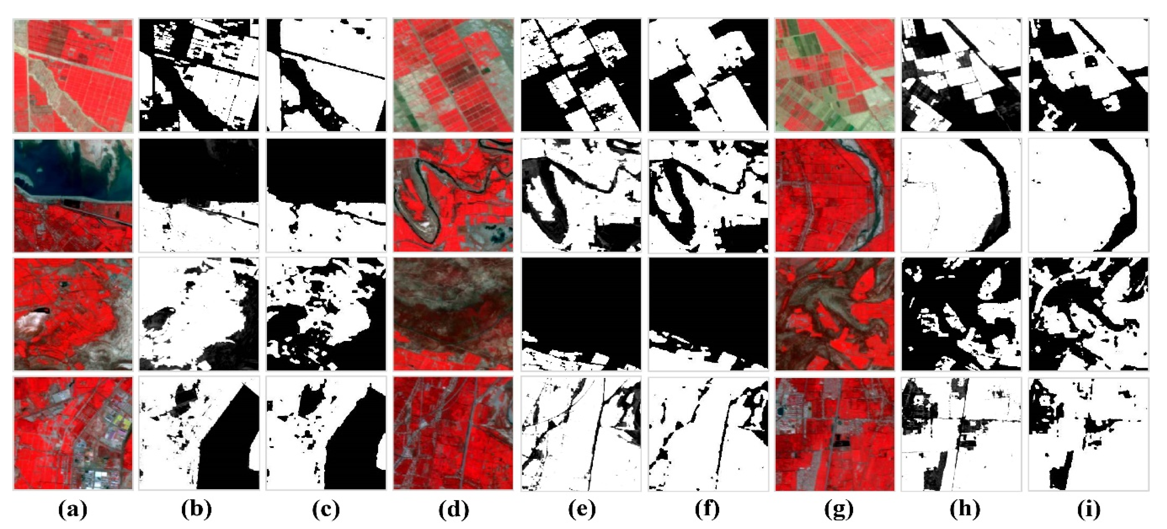
4.3. Cotton Crop Identification

The matrices of P, R, F1, and mIoU are used to evaluate CNN models’ applicability, including DenseNet, ResNet, VGG, SegNet, and DeepLab v3+, on cotton identification task from both quantitative and qualitative perspectives. By comparing the predictions of the 3300 test images with the corresponding ground truths, we have derived the statistics of the four matrices and tabulated them in

Table 3. The derived P, R, F1 score and mIoU of the VGG, ResNet, DenseNet, SegNet, DeepLab v3+ models with 95% confidence interval. The optimal value for each metric is boldened.

	DenseNet	ResNet	VGG	SegNet	DeepLab v3+
P	0.948 ± 0.008	0.875 ± 0.011	0.912 ± 0.010	0.907 ± 0.010	0.892 ± 0.011
R	0.960 ± 0.007	0.881 ± 0.011	0.937 ± 0.008	0.971 ± 0.006	0.950 ± 0.007
F1	0.953 ± 0.007	0.878 ± 0.011	0.924 ± 0.009	0.938 ± 0.008	0.920 ± 0.009
mIoU	0.911 ± 0.010	0.783 ± 0.014	0.860 ± 0.012	0.883 ± 0.011	0.853 ± 0.012

. Considering the limited samples, the metrics’ 95% confidence interval shows their significance. The boldened values indicated the optimal values of evaluation matrices. The DenseNet appears to have the highest precision value of 0.948, indicating that the model correctly predicts 94.8% of the cotton crop samples. However, the ResNet suffers a heavy breakdown on the cotton crop identification, whose precision is 87.5%. The precision of VGG, SegNet and DeepLab v3+ are 0.912, 0.907 and 0.892, respectively. As a result, the DenseNet significantly outperforms the other models concerning the prediction precision. It is also indicated that the DenseNet result is more robust with a narrower confidence interval than the other models. However, the SegNet shows the highest recall value of 0.971, followed by the DenseNet with a value of 0.960. The recall values of ResNet, VGG and DeepLab v3+ are 0.881, 0.937 and 0.950 respectively. The ResNet performs relatively lower regarding both precision and recall values.

We further introduce the F1 score, which takes into account both recall and precision values simultaneously. Furthermore, the mIoU is investigated to evaluate the accuracy of segmentation consequences. Higher F1 or mIoU value indicates better model performance. From Table 3, the F1 scores of DenseNet, ResNet, VGG, SegNet and DeepLab v3+ are 0.953, 0.878, 0.924, 0.938 and 0.920; and their mIoU values are 0.911, 0.783, 0.860, 0.883 and 0.853, respectively. The DenseNet outperforms the other four models regarding F1 and mIoU matrices.

Among the matrics of P, R, F1, and mIoU, the DenseNet performs the best regarding P, F1, and mIoU; and it ranks the second for R. Therefore, the DenseNet can be concluded to have the best performance for the cotton identification task in our study when considering the general probability. This is probably due to the used dense connection structure, which makes full and efficient use of all layers’ image features. In addition to the above evaluation metrics, It is important to understand the model performance in detail through result visualization. Therefore, we selected the GF-1 images of Wei-Ku oasis on 21 September 2018, to exhibit each model’s overall performance. We stitched the predicted small images according to the original ground truth image’s geographic location to obtain a large-scale binary map, which achieves the purpose of predicting the cotton distribution in a wide range.

Figure 5 is the overall map demonstrating the cotton prediction results by DenseNet (Figure 5b), ResNet (Figure 5c), VGG (Figure 5d), SegNet (Figure 5e), and DeepLab v3+ (Figure 5f) models. It is noteworthy that we added some noise, such as mountain shadows, to avoid confusion and misjudgment in the preprocessing pipeline. In the false-color composite image, the cotton fields are shown in red. We can see that the DenseNet predictions are the most consistent with the original image, while the ResNet and VGG predictions are relatively rough. From the visual interpretation, the performance of DenseNet is better than the other models on the discrimination between cotton and non-cotton fields, without excessive confusion and misjudgment. Misjudgment occurs where there are mountain shadows; however, this does not happen to the DenseNet model. The cotton predictions by the DenseNet have shown clear texture and contours; however, predictions by the other models are blurred, and their edges are broken. From these observations, the DenseNet appears better to identify the cotton fields from the whole image, especially avoiding mountain shadows’ misjudgments.

Affected by the surrounding environment, cotton fields were over-identified in intricate and interstitial places, and some other small features were not excluded.

Figure 6 shows six selected subimages mixed, including river, city, mountain, and cotton fields, and the results derived from the different models. Compared with the ground truth, the DenseNet models shows rather better performance than the other four models in these places, with a quite less falsely identified cotton crop. This outperformance is particularly true where there are mountain shadows or small river systems. P-value is likely to be reduced if we attempt to improve the R-value of DenseNet. Concerning the F1 score and mIoU results, the overall performance of DenseNet is ideal. Thus, we desisted from making further optimizations on the R of this network. Nevertheless, the recognition effect of Densenet is the best of these five models.

As shown above, the DenseNet (Figure 6c) is superior to the ResNet (Figure 6d), the VGG (Figure 6e), the SegNet (Figure 6f), and the DeepLab v3+ (Figure 6g) models in identifying cotton crop. However, it is still not sufficiently credible only by comparing the performances of different models; and we have further evaluated the DenseNet credibility with 12 subimages from different locations.

We visualize the detailed features of 12 subimages, the corresponding ground truths (Figure 7b,e,h), and the DenseNet (Figure 7c,f,i) predictions from the validation dataset, shown in Figure 7. These subimages have a uniform size of 224 × 224 pixels, and each pixel refers to 16 m for both length and width. The identification results appear consistent with the ground truths, indicating the good performance of the DenseNet model in identifying the fine structure of cotton fields. The subimages in the first row of Figure 7 have cotton fields with different shapes and false colors, which are rather accurately identified by the DenseNet model. The subimages in the second row contain water bodies of rivers and ponds; the cotton fields are successfully distinguished from them. There are clouds and mountain shadows in the subimages of the third row, and they are not wrongly identified as cotton fields. In the last row, the subimages contain large urban areas, and the DenseNet model can distinguish the cotton fields from them successfully.

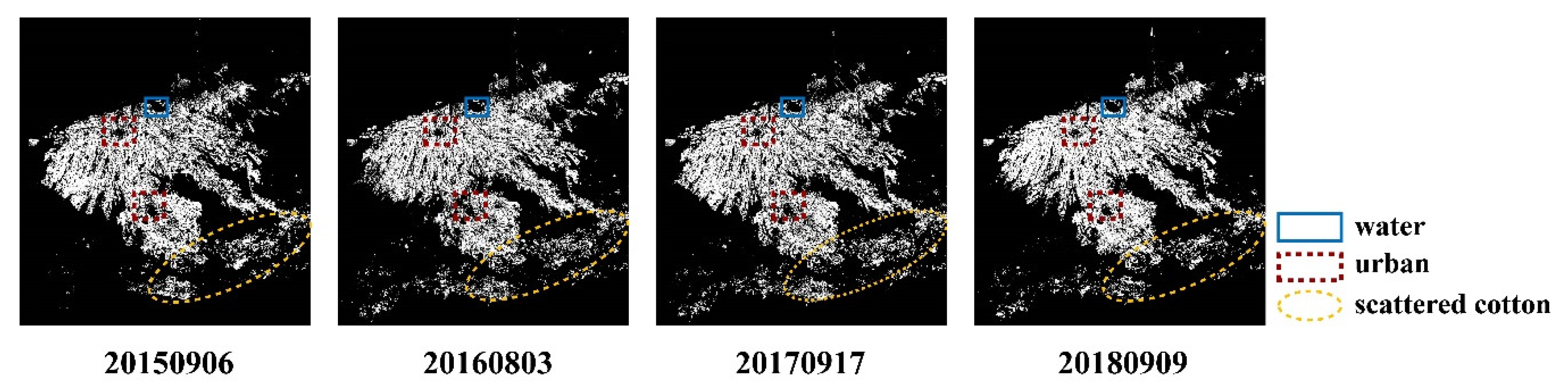
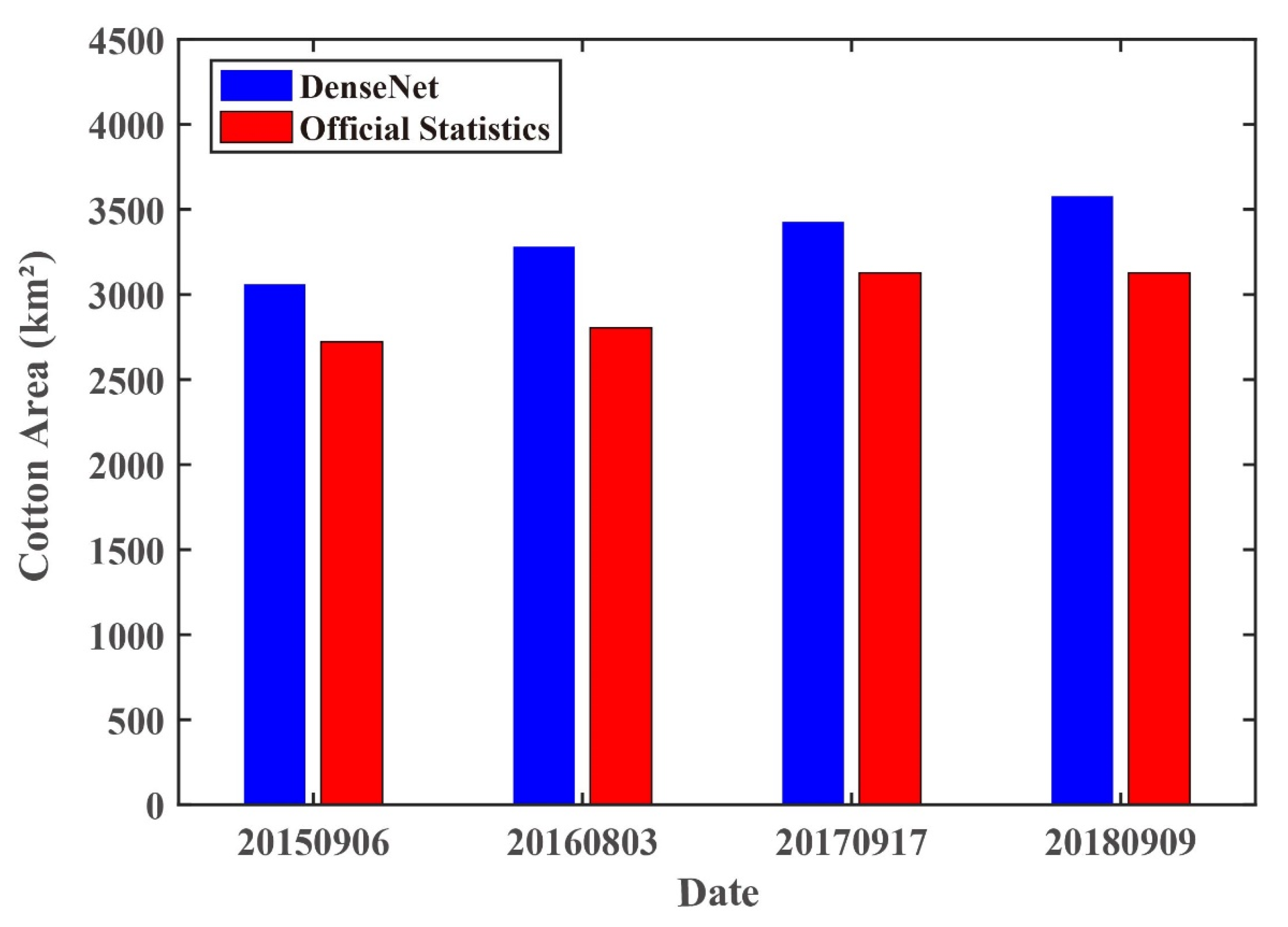
4.4. Interannual Variations of Cotton Cultivated Fields

From the above analysis, it can be concluded that the improved DenseNet model we introduced has better results and can be used for cotton field identification. Therefore, we intended to use this model to explore the interannual changes of cotton cultivated areas of Wei-ku Oasis. Due to GF-1 post-2013 data provision and lack of data for the study area in 2014, we could only discuss changes in the cotton crop cultivated area from 2015 to 2018 (Figure 8). The cotton cultivated areas of Wei-ku Oasis change not vary significantly among years. The main difference comes from the scattered cotton fields in the south, near towns and water bodies, mainly related to human activities. With limited temporal imageries, we can still locate and report changes in the spatio-temporal pattern of the cotton crop area, highlighting the potential of the improved DenseNet model efficiently not only for cotton crop identification but also for accurate spatiao-temporal change assessment. Generally speaking, the cultivated cotton area does not vary greatly from year to year unless extreme events occur. To prove the credibility of the recognition results, based on the satellite’s spatial resolution and pixel number, we made statistics of the identified cotton field area and compared them with the actual statistical data from the local statistical yearbook. Since the Wei-Ku Oasis is mainly composed of Kuche, Xinhe, and Shaya County, we add the three counties’ data as the sown area’s official statistics in this region.

Figure 9 shows the interannual variations of cotton crop cultivated areas of Wei-Ku Oasis, derived from GF-1 images from 2015 to 2018 based on the DenseNet model. According to statistics, the cultivated cotton area in Wei-Ku region showed a growing trend from 2015 to 2018, with all more than 3000 km². In 2018, the area was the largest, with more than 3500 km². Combined with

Table 4. Comparison of total cultivated cotton acreage from 2015–2018 based on DenseNet estimation and the official statistics (expressed in km²).

Year	DenseNet	Official Statistics	Difference
2015	3060.32	2722.20	+338.12
2016	3281.40	2804.70	+476.70
2017	3427.58	3127.60	+299.98
2018	3578.26	3127.60	+450.66

, it can be seen that the cotton field area identified by the DenseNet model is overestimated compared to official statistics, and the difference is between 300 and 500 km². The biggest difference was in 2016, up to 476.70 km², the smallest difference was in 2017, only 300 km². The official statistics are obtained using interviews or investigation and reporting level by level, which is highly subjective and lacks scientific rigor. However, compared with other studies in this area, only the Landsat TM images in 2011 were used for cotton cropland remote sensing monitoring and area statistics. This study shows that precision and difference is 94.77% and +77.17 km^2, respectively [63]. This difference can be many kinds of crops and complex planting structure in Wei-Ku oasis. The identification of cotton and other crops is easy to be misclassified, which leads to the reduction of cotton information extraction accuracy. Previous studies are also based on a large number of field survey results, naturally have high accuracy, but time-consuming, low application value. Our research can be based on remote sensing images to achieve rapid and efficient identification of cotton field for the subsequent yield estimation application to buy time. Therefore, although the remote sensing techniques differ from the actual statistical data, the overall trend is consistent, scientific, and reliable. Thus, the results of cotton field identification based on the improvement DenseNet model are credible and have application value.

5. Discussion and Conclusions

This study used the improved DenseNet structure, which was used for water identification previously [53], to identify cotton fields using GF-1 multispectral images. This model can introduce feature fusion into deep feature extraction, which conducts image down-sampling and then uses trans-convolution for image up-sampling. On this basis, multiscale fusion is added to aggregate features of different scales in the down-sampling process into the upsampling process. With the advantage of a faculty of convolution layers that handle multi-dimensional data, the model can fully use both spatial and spectral information for cotton field identification. The DenseNet results have been validated using ground truths and compared with four popular CNNs of ResNets, VGG, SegNet, and DeepLab v3+. According to the experimental results, the improved DenseNet model is superior to these popular CNNs using the same datasets. The DenseNet model shows definite capability in distinguishing cotton fields from mountain shadows, water bodies, towns, bare land, clouds, etc. The study has suggested that a deep neural network architecture built with the DenseNet is a reliable option among the widely-used multi-spectral classification tasks. It can be seen from cotton cultivated area changes in the recent years that the derived cotton field areas from the deep learning method can well reflect cotton planting conditions and make up for the deficiency of manual statistics. Therefore, using the improved DenseNet method, the changes in cotton fields, even other cropland can be timely and effectively monitored.

A future task will be to verify the improved DenseNet model on images with higher temporal, spatial, and spectral resolutions for cotton field identification [64]. With the rapid development of UAV (Unmanned Aerial Vehicle) [65], we can also utilize its data resource to realize the fine cotton field and also cotton disease detection for precision agriculture [66,67]. Such an efficient deep learning network can be developed into a fully automated process system with remote sensing big data and is feasible in smart agriculture [68,69].

References

1. Gao, W.; Han, R. Xin Jiang Stastical Yearbook, 3rd ed.; China Statistics Publishing House: Beijing, China, 2019; pp. 287–346.
2. China Cotton: Record Yield. Available online: http://www.pecad.fas.usda.gov/cropexplorer/ (accessed on 1 December 2017).
3. Li, N.; Lin, H.; Wang, T.; Li, Y.; Liu, Y.; Chen, X.; Hu, X. Impact of climate change on cotton growth and yields in Xinjiang, China. Field Crops Res. 2019, 247, 107590. [Google Scholar] [CrossRef]
4. Chen, X.; Qi, Z.; Gui, D.; Gu, Z.; Ma, L.; Zeng, F.; Li, L. Simulating impacts of climate change on cotton yield and water requirement using RZWQM2. Agric. Water Manag. 2019, 222, 231–241. [Google Scholar] [CrossRef]
5. Shao, Y.; Fan, X.; Liu, H.; Xiao, J.; Ross, S.; Brisco, B.; Brown, R.; Staples, G. Rice monitoring and production estimation using multitemporal RADARSAT. Remote Sens. Environ. 2011, 76, 310–325. [Google Scholar] [CrossRef]
6. Franch, B.; Vermote, E.F.; Becker-Reshef, I.; Claverie, M.; Huang, J.; Zhang, J.; Justice, C.; Sobrino, J.A. Improving the timeliness of winter wheat production forecast in the United States of America, Ukraine and China using MODIS data and NCAR Growing Degree Day information. Remote Sens. Environ. 2015, 161, 131–148. [Google Scholar] [CrossRef]
7. Atzberger, C. Advances in Remote Sensing of Agriculture: Context Description, Existing Operational Monitoring Systems and Major Information Needs. Remote Sens. 2013, 5, 949–981. [Google Scholar] [CrossRef] [Green Version]
8. Franke, J.; Menz, G. Multi-temporal wheat disease detection by multi-spectral remote sensing. Precis. Agric. 2007, 8, 161–172. [Google Scholar] [CrossRef]
9. Wang, X.; Huang, J.; Feng, Q.; Yin, D. Winter Wheat Yield Prediction at County Level and Uncertainty Analysis in Main Wheat-Producing Regions of China with Deep Learning Approaches. Remote Sens. 2020, 12, 1744. [Google Scholar] [CrossRef]
10. Pradhan, S. Crop area estimation using GIS, remote sensing and area frame sampling. Int. J. Appl. Earth Obs. Geoinf. 2001, 3, 86–92. [Google Scholar] [CrossRef]
11. Tellaeche, A.; Pajares, G.; Burgos-Artizzu, X.P.; Ribeiro, A. A computer vision approach for weeds identification through Support Vector Machines. Appl. Soft Comput. 2011, 11, 908–915. [Google Scholar] [CrossRef] [Green Version]
12. Weiss, M.; Jacob, F.; Duveiller, G. Remote sensing for agricultural applications: A meta-review. Remote Sens. Environ. 2020, 236, 111402. [Google Scholar] [CrossRef]
13. Nitze, I.; Schulthess, U.; Asche, H. Comparison of machine learning algorithms random forest, artificial neural network and support vector machine to maximum likelihood for supervised crop type classification. In Proceedings of the 4th GEOBIA, Rio de Janeiro, Brazil, 7–9 May 2012; p. 35. [Google Scholar]
14. Chen, S.; Zhao, Y.; Shen, S. Crop classification by remote sensing based on spectral analysis. Trans. Chin. Soc. Agric. Eng. 2012, 28, 154–160. [Google Scholar]
15. Bischof, H.; Schneider, W.; Pinz, A.J. Multispectral classification of Landsat-images using neural networks. IEEE Trans. Geosci. Remote Sens. 1992, 30, 482–490. [Google Scholar] [CrossRef]
16. Laban, N.; Abdellatif, B.; Ebeid, H.M.; Shedeed, H.A.; Tolba, M.F. Machine Learning for Enhancement Land Cover and Crop Types Classification. In Machine Learning Paradigms: Theory and Application; Hassanien, A., Ed.; Studies in Computational Intelligenc; Springer: Cham, Switzerland, 2019; Volume 801, pp. 71–87. [Google Scholar]
17. Jamuna, K.S.; Karpagavalli, S.; Vijaya, M.S.; Revathi, P.; Gokilavani, S.; Madhiya, E. Classification of Seed Cotton Yield Based on the Growth Stages of Cotton Crop Using Machine Learning Techniques. In Proceedings of the International Conference on Advances in Computer Engineering, Bangalore, India, 20–21 July 2010; pp. 312–315. [Google Scholar]
18. Mathur, A.; Foody, G.M. Crop classification by support vector machine with intelligently selected training data for an operational application. Int. J. Remote Sens. 2018, 29, 2227–2240. [Google Scholar] [CrossRef] [Green Version]
19. Ishak, A.J.; Tahir, N.M.; Hussain, A.; Mustafa, M.M. Weed classification using Decision Tree. In Proceedings of the the IEEE Conference on International Symposium on Information Technology, Kuala Lumpur, Malaysia, 26–28 August 2008. [Google Scholar]
20. Roy, P.S.; Behera, M.D.; Srivastav, S.K. Satellite Remote Sensing: Sensors, Applications and Techniques. Proc. Natl. Acad. Sci. India Sect. A Phys. Sci. 2017, 87, 465–472. [Google Scholar] [CrossRef] [Green Version]
21. Zhang, W.; Liu, C.; Chang, F.; Song, Y. Multi-Scale and Occlusion Aware Network for Vehicle Detection and Segmentation on UAV Aerial Images. Remote Sens. 2020, 12, 1760. [Google Scholar] [CrossRef]
22. Phan, C.; Liu, H.H.T. A cooperative UAV/UGV platform for wildfire detection and fighting. In Proceedings of the IEEE Conference on Asia Simulation Conference-international Conference on System Simulation & Scientific Computing, Beijing, China, 10–12 October 2008. [Google Scholar]
23. Viswanathan, B.; Pires, R.; Huber, D. Vision based robot localization by ground to satellite matching in GPS-denied situations. In Proceedings of the 2014 IEEE/RSJ International Conference on Intelligent Robots and Systems, Chicago, IL, USA, 14–18 September 2014; pp. 192–198. [Google Scholar]
24. Gong, P.; Liu, H.; Zhang, M.; Li, C.; Wang, J.; Huang, H.; Clinton, N.; Ji, L.; Li, W.; Bai, Y.; et al. Stable classification with limited sample: Transferring a 30-m resolution sample set collected in 2015 to mapping 10-m resolution global land cover in 2017. SCIB 2019, 19, 2095–9273. [Google Scholar] [CrossRef] [Green Version]
25. Li, C.; Gong, P.; Wang, J.; Yuan, C.; Hu, T.; Wang, Q.; Yu, L.; Clinton, N.; Li, M.; Guo, J.; et al. An all-season sample database for improving land-cover mapping of Africa with two classification schemes. Int. J. Remote Sens. 2016, 37, 4623–4647. [Google Scholar] [CrossRef]
26. Maggiori, E.; Tarabalka, Y.; Charpiat, G.; Alliez, P. Convolutional Neural Networks for Large-Scale Remote-Sensing Image Classification. IEEE Trans. Geosci. Electron. 2017, 55, 645–657. [Google Scholar] [CrossRef] [Green Version]
27. Kussul, N.; Lavreniuk, M.; Skakun, S.; Shelestov, A. Deep Learning Classification of Land Cover and Crop Types Using Remote Sensing Data. IEEE Trans. Geosci. Remote Sens. 2017, 14, 778–782. [Google Scholar] [CrossRef]
28. Zhang, L.; Liu, Z.; Ren, T.; Liu, D.; Ma, Z.; Tong, L.; Zhang, C.; Zhou, T.; Zhang, X.; Li, S. Identification of seed maize fields with high spatial resolution and multiple spectral remote sensing using random forest classifier. Remote Sens. 2020, 12, 362. [Google Scholar] [CrossRef] [Green Version]
29. Liu, W.; Wang, Z.; Liu, X.; Zeng, N.; Liu, Y.; Alsaadi, F.E. A survey of deep neural network architectures and their applications. Neurocomputing 2017, 234, 11–26. [Google Scholar] [CrossRef]
30. Kamilaris, A.; Francesc, X.; Boldú, P. Deep learning in agriculture: A survey. Comput. Electron. Agric. 2018, 147, 70–90. [Google Scholar] [CrossRef] [Green Version]
31. Zhang, X.; Xv, C.; Shen, M.; He, X.; Du, W. Survey of Convolutional Neural Network. In Proceedings of the 2018 International Conference on Network, Communication, Computer Engineering (NCCE 2018), Chongqing, China, 1 January 2017. [Google Scholar]
32. Krizhevsky, A.; Sutskever, I.; Hinton, G.E. ImageNet Classification with Deep Convolutional Neural Networks. In Proceedings of the Neural Information Processing Systems, Lake Tahoe, NV, USA, 3–6 December 2012; pp. 1097–1105. [Google Scholar]
33. Simonyan, K.; Zisserman, A. Very Deep Convolutional Networks for Large-Scale Image Recognition. Available online: https://www.arxiv-vanity.com/papers/1409.1556/ (accessed on 18 December 2019).
34. He, K.; Zhang, X.; Ren, S.; Sun, J. Deep Residual Learning for Image Recognition. In Proceedings of the IEEE Conference on Computer Vision and Pattern Recognition, Las Vegas, NV, USA, 26–30 June 2016; pp. 770–778. [Google Scholar]
35. Huang, G.; Liu, Z.; van Maaten, L.; Weinberger, K.Q. Densely Connected Convolutional Networks. In Proceedings of the IEEE Conference on Computer Vision and Pattern Recognition, Honolulu, HI, USA, 21–26 July 2017; pp. 2261–2269. [Google Scholar]
36. Feng, M.; Sexton, J.O.; Channan, S.; Townshend, J.R. A global, 30-m resolution land-surface water body dataset for 2000: First results of a topographic-spectral classification algorithm. Int. J. Digit. Earth 2016, 9, 113–133. [Google Scholar] [CrossRef] [Green Version]
37. Sabit, M.; Jiang-Ling, H.U.; Ismail, D. Climatic Change Characteristics of Kuqa River-Weigan River Delta Oasis during Last 40 Years. Entia Geogr. Sin. 2008, 28, 518–524. [Google Scholar]
38. Förstner, W. Image Preprocessing for Feature Extraction in Digital Intensity, Color and Range Images. In Geomatic Method for the Analysis of Data in the Earth Sciences; Dermanis, A., Grün, A., Sansò, F., Eds.; Springer: Berlin/Heidelberg, Germany, 2000; Volume 95. [Google Scholar]
39. Cui, X.; Goel, V.; Kingsbury, B. Data augmentation for deep convolutional neural network acoustic modeling. In Proceedings of the 2015 IEEE International Conference on Acoustics, Speech and Signal Processing (ICASSP), Brisbane, QLD, Australia, 19–24 April 2015; pp. 4545–4549. [Google Scholar]
40. Girshick, R.; Donahue, J.; Darrel, T.; Malik, J. Rich Feature Hierarchies for Accurate Object Detection and Semantic Segmentation. Available online: https://arxiv.org/abs/1311.2524 (accessed on 10 February 2020).
41. Girshick, R. Fast R-CNN. In Proceedings of the International Conference on Computer Vision, Santiago, MN, USA, 13–16 December 2015; pp. 1440–1448. [Google Scholar]
42. Ren, S.; He, K.; Girshick, R.; Sun, J. Faster R-CNN: Towards Real-Time Object Detection with Region Proposal Networks. In Advances in Neural Information Processing Systems 28; Cortes, C., Lawrence, N.D., Lee, D.D., Sugiyama, M., Garnett, R., Eds.; Curran Associates, Inc.: Red Hook, NY, USA, 2015. [Google Scholar]
43. He, K.; Gkioxari, G.; Dollar, P.; Girshick, R. Mask R-CNN. Available online: https://arxiv.org/abs/1703.06870 (accessed on 10 February 2020).
44. Chen, K.; Pang, J.; Wang, J.; Xiong, Y.; Li, X.; Sun, S.; Feng, W.; Liu, Z.; Shi, J.; Ouyang, W.; et al. Hybrid Task Cascade for Instance Segmentation. Available online: https://arxiv.org/abs/1901.07518 (accessed on 19 February 2020).
45. Chen, L.; Yang, Y.; Wang, J.; Xu, W.; Yuille, A.L. Attention to Scale: Scale-Aware Semantic Image Segmentation. In Proceedings of the IEEE Conference on Computer Vision and Pattern Recognition, Las Vegas, NV, USA, 26–30 June 2016; pp. 3640–3649. [Google Scholar]
46. Fu, J.; Liu, J.; Tian, H.; Li, Y.; Bao, Y.; Fang, Z.; Lu, H. Dual attention network for scene segmentation. In Proceedings of the IEEE Conference on Computer Vision and Pattern Recognition, Long Beach, CA, USA, 16–20 June 2019; pp. 3146–3154. [Google Scholar]
47. Marquez-Neila, P.; Baumela, L.; Alvarez, L. A Morphological Approach to Curvature-Based Evolution of Curves and Surfaces. IEEE Trans. Pattern Anal. Mach. Intell. 2014, 36, 2–17. [Google Scholar] [CrossRef]
48. Minaee, S.; Boykov, Y.; Porikli, F.; Plaza, A.; Kehtarnavaz, N.; Terzopoulos, D. Image Segmentation Using Deep Learning: A Survey. Available online: https://arxiv.org/abs/2001.05566 (accessed on 19 February 2020).
49. Lecun, Y.; Bottou, L.; Bengio, Y.; Haffner, P. Gradient-based learning applied to document recognition. Proc. IEEE 1998, 86, 2278–2324. [Google Scholar] [CrossRef] [Green Version]
50. Zhang, C.; Xie, Y.; Liu, D.; Wang, L. Fast Threshold Image Segmentation Based on 2D Fuzzy Fisher and Random Local Optimized QPSO. IEEE Trans. Image Process. 2017, 26, 1355–1362. [Google Scholar] [CrossRef]
51. Erhan, D.; Szegedy, C.; Toshev, A.; Anguelov, D. Scalable Object Detection using Deep Neural Networks. In Proceedings of the IEEE Conference on Computer Vision and Pattern Recognition, Columbus, OH, USA, 24–27 June 2014; pp. 2155–2162. [Google Scholar]
52. Huang, G.; Sun, Y.; Liu, Z.; Sedra, D.; Weinberger, K. Deep Networks with Stochastic Depth. In Proceedings of the European Conference on Computer Vision, Amsterdam, The Netherlands, 10–16 October 2016; pp. 646–661. [Google Scholar]
53. Wang, G.; Wu, M.; Wei, X.; Song, H. Water Identification from High-Resolution Remote Sensing Images Based on Multidimensional Densely Connected Convolutional Neural Networks. Remote Sens. 2020, 12, 795. [Google Scholar] [CrossRef] [Green Version]
54. Long, J.; Shelhamer, E.; Darrell, T. Fully convolutional networks for semantic segmentation. In Proceedings of the IEEE Conference on Computer Vision and Pattern Recognition, Boston, MA, USA, 7–12 June 2015; pp. 3431–3440. [Google Scholar]
55. Srivastava, R.K.; Greff, K.; Schmidhuber, J. Highway Networks. Available online: https://arxiv.org/abs/1505.00387 (accessed on 15 December 2019).
56. Larsson, G.; Maire, M.; Shakhnarovich, G. FractalNet: Ultra-Deep Neural Networks without Residuals. Available online: https://arxiv.org/abs/1605.07648 (accessed on 15 December 2019).
57. Kingma, D.P.; Ba, J. Adam: A Method for Stochastic Optimization. Available online: https://arxiv.org/abs/1412.6980 (accessed on 10 October 2019).
58. Badrinarayanan, V.; Kendall, A.; Clipolla, R. A Deep Convolutional Encoder-Decoder Architecture for Image Segmentation. IEEE Trans. Pattern Anal. Mach. Intell. 2017, 39, 2481–2495. [Google Scholar] [CrossRef]
59. Chen, L.C.; Papandreou, G.; Kokkinos, I.; Murphy, K.; Yuille, A.L. DeepLab: Semantic Image Segmentation with Deep Convolutional Nets, Atrous Concolution, and Fully Connected CRFs. Available online: https://arxiv.org/abs/1606.00915 (accessed on 10 February 2020).
60. Powers, D.M.W. Evaluation: From Precision, Recall and F-Measure to ROC, Informedness, Markedness & Correlation. J. Mach. Learn. Technol. 2011, 2, 37–63. [Google Scholar]
61. Wu, Z.; Shen, C.; Van, A.; Henge, D. Wider or Deeper: Revisiting the ResNet Model for Visual Recognition. Pattern Recognit. Lett. 2019, 90, 119–133. [Google Scholar] [CrossRef] [Green Version]
62. Howard, A.G.; Zhu, M.; Chen, B.; Kalenichenko, D.; Wang, W.; Weyand, T.; Andreetto, M.; Adam, H. MobileNets: Efficient Convolutional Neural Networks for Mobile Vision Applications. Available online: https://arxiv.org/abs/1704.04861 (accessed on 10 December 2019).
63. Yusup, M.; Tursun, H.; Magpirat, G. Remote Sensing of Cotton Plantation Areas Monitoring in Delta Oasis of Ugan-Kucha River, Xinjiang. Res. Agric. Modern. 2014, 35, 240–243. [Google Scholar]
64. Yao, C.; Zhang, Y.; Liu, H. Application of convolutional nerual network in classification of high resolution agricultural remote sensing images ISPRS. Remote Sens. Spat. Inf. Sci. 2017, 42, 989–992. [Google Scholar]
65. Lottes, P.; Khanna, R.; Pfeifer, J.; Siegwart, R.; Stachniss, C. UAV-based crop and weed classification for smart farming. In Proceedings of the IEEE International Conference on Robotics and Automation (ICRA), Singapore, 29 May–3 June 2017; pp. 3024–3031. [Google Scholar]
66. Zhang, X.; Sun, Y.; Shang, K.; Zhang, L.; Wang, S. Crop Classification Based on Feature Band Set Construction and Object-Oriented Approach Using Hyperspectral Images. IEEE J. Sel. Top. Appl. Earth Obs. Remote Sens. 2016, 9, 4117–4128. [Google Scholar] [CrossRef]
67. Sharada, P.; Hughes, D.P.; Salathé, M. Using Deep Learning for Image-Based Plant Disease Detection. Front. Recent Dev. Plant Sci. 2016, 7, 1419. [Google Scholar]
68. Bendre, M.R.; Thool, R.C.; Thool, V.R. Big data in precision agriculture: Weather forecasting for future farming. In Proceedings of the at 1st International Conference on Next Generation Computing Technologies (NGCT), Dehradun, India, 4–5 September 2015; pp. 744–750. [Google Scholar]
69. Erives, H.; Fitzgerald, G.J. Automated registration of hyperspectral images for precision agriculture. Comput. Electron. Agric. 2015, 47, 103–119. [Google Scholar] [CrossRef]
Figure 1. The geographical location of the study area.
Agronomy 11 00174 g001
Figure 2. Multi-dimensional Dense Connection Module (BN refers to batch normalization, ReLU refers to rectified linear unit, Conv refers to convolution).
Agronomy 11 00174 g002
Figure 3. The improved network architecture of semantic identification based on the DenseNet model.
Agronomy 11 00174 g003
Figure 4. The training losses of the DenseNet, the ResNet, the VGG, the SegNet, and the DeepLab v3+ models. One epoch represents 1000 iterations.
Agronomy 11 00174 g004
Figure 5. Comparison of the cotton identification effect of different models in Wei-Ku oasis on 21 September 2018. (a) False color composite remote sensing images, and cotton identification result by (b) the DenseNet, (c) the ResNet, (d) the VGG, (e) the SegNet, and (f) the DeepLab v3+. The white color indicates the identified cotton, the yellow solid line depicts mountain area, and the yellow dashed line depicts cloud area.
Agronomy 11 00174 g005
Figure 6. Cotton identification results from six subimages by different models; (a) the false color composite subimages, (b) the cotton ground truth, and the cotton identification results by (c) the DenseNet, (d) the ResNet, (e) the VGG, (f) the SegNet and (g) the DeepLab v3+ respectively. The white color indicates the identified cotton fields.
Agronomy 11 00174 g006
Figure 7. The cotton identification results from 12 subimages by the DenseNet model. The figure is divided into four rows and nine columns. Columns (a,d,g) are the false color subimages; column (b,e,h) are the corresponding ground truths; column (c,f,i) are the DenseNet predictions.
Agronomy 11 00174 g007
Figure 8. The spatial variations of cotton field cultivated area from 2015–2018 in Wei-Ku Oasis based on DenseNet.
Agronomy 11 00174 g008
Figure 9. Statistics on the change of cotton field cultivated area from 2015 to 2018 in Wei-ku Oasis, derived from GF-1 images.
Agronomy 11 00174 g009