Article

Estimation of Sensible and Latent Heat Fluxes Using Surface Renewal Method: Case Study of a Tea Plantation

1
School of Agricultural Engineering, Jiangsu University, Zhenjiang 212013, China
2
Department of Irrigation and Drainage, University of Agriculture, Faisalabad 3800, Pakistan
*
Author to whom correspondence should be addressed.
Submission received: 26 November 2020 / Revised: 2 January 2021 / Accepted: 14 January 2021 / Published: 18 January 2021
(This article belongs to the Special Issue Agricultural Water Conservation: Tools, Strategies, and Practices)

Abstract

:
An experiment of sensible and latent heat flux measurement was conducted in a tea plantation near the Yangtze River within Danyang of Jiangsu Province, China. High-frequency (~10 Hz) air temperature measurement with fine-wire thermocouples (⌀ = 50 μm) was used for the estimation of sensible heat flux (H), and latent heat flux (LE) was extracted as a residual of the energy balance equation using additional measurements of net radiation (Rn) and soil heat flux (G). Results were compared against the eddy covariance (EC) system under unstable conditions only, and days with high precipitation were excluded from further analysis. Half-hourly datasets of the sensible heat flux estimated using the surface renewal method (SR) (HSR) and measured by the EC system (HEC) were analyzed. Results showed good agreement with R2 = 0.80, root mean square error (RMSE) = 27.87 W m−2, relative error (RE) = 9.02%, and a regression slope of 0.68—this slope was used for the calibration of the uncalibrated HSR estimated by SR. On the other hand, the half-hourly dataset of LESR was regressed against EC, and it showed good agreement with relatively high R2 = 0.93, RMSE = 32.99 W·m−2, and RE = 5.67%. Hence, the SR method may estimate the surface fluxes at a relatively low cost, ultimately improving calculations of evapotranspiration. Thus, the SR method could provide an economical tool for improving crop water management of tea plantations.

1. Introduction

Latent heat flux (LE) measurement is very critical in the field of micrometeorology for the efficient management of available water resources. The precise estimation of LE, also termed as evapotranspiration (ET), is vital due to its great influence on precipitation, plant growth, and amount of irrigation water runoff. There is constant pressure on the available water resources for different crops in arable agricultural areas. Therefore, there is always a need for accurate estimation of crop evaporation to maximize the available water resources and crop water use efficiency. Traditionally, crop water evaporation was estimated from climatic data and reference evapotranspiration methods and by using the crop coefficient approach [1]. In recent decades, the instrumentation, techniques, and different approaches for the estimation of ET have been improved a lot. In order to spread scientifically approved techniques into commercial practice, simpler techniques are preferred. Various micrometeorological methods have been used for estimating LE (i.e., scintillometer, eddy covariance (EC), Bowen ratio (BR) [2], lysimeter, surface renewal (SR), and flux variance (FV)) [3]. Use of a lysimeter is a reliable method for ET measurements, but it is seldom used outside of experimental stations [4,5]. The Bowen ratio (BR) method requires extensive fetch and responsiveness to the biases of the instrument used for estimating the air temperature and water vapor pressure at two levels [2]. The scintillometer method is a high-cost method based on the Monin–Obukhov similarity theory (MOST) and high skills are required for correct operation. In addition, its estimations are disrupted by optical interception of rainfall, insects, frost, and vertical air temperature to differentiate between the ascending and descending directions of sensible heat flux (H) [6]. The EC system allows the direct measurement of surface fluxes (sensible and latent heat fluxes), and a lysimeter can also provide estimations of these fluxes with better accuracy. In spite of their many advantages, these techniques are not easily available for daily usage by farmers due to high cost and operational complexity; hence, simple and low-cost methods for ET measurement are required [7]. There are few studies of ET estimation over different homogeneous surfaces and crops using these methods. Most of these methods are costly and their instrumentation is sensitive to damage, requiring site homogeneity and relatively wide fetch. The SR method has been proposed as a reliable alternative to methods such as the EC system, first proposed by Van Atta in 1977 [8]. The theoretical basics of the SR method have been reviewed and applied over different crop canopies and surfaces with better results [9,10,11,12,13,14,15,16]. The SR method uses high-frequency (~10 Hz) air temperature measurements obtained from fine-wire thermocouples for the estimation of the sensible heat flux (H) above the plant canopy. The SR method has been deployed over natural surfaces with mixed results and is considered as an attractive replacement for other available meteorological methods due to its low-cost and relatively simple instrumentation, which makes it easier to apply close to the canopy surface and with limited fetch [17,18,19].
This study tests the performance of the surface renewal method for estimating the surface fluxes, including sensible and latent heat fluxes, over a tea plantation in Danyang. Tea plants grow well all year round in temperate and humid climates. During the last decade, sprinkling irrigation has been gradually applied to tea plantations and drip irrigation has been recently adopted with the extension of fertigation technology. Usually, growers start irrigation based on only soil moisture content, without knowing the exact crop water requirement [20]. This study was performed with the aim to provide a relatively low-cost technique for estimation of the crop water requirement of tea plants. The performance of the SR method was evaluated for the estimation of surface fluxes including sensible and latent heat fluxes and the results were compared against the measurements of the eddy covariance system.

2. Materials and Methods

2.1. Study Site and Climate

The experiment was conducted at a tea plantation located in Danyang, Jiangsu, P.R China (32.026177° N, 119.674201° E), at an elevation of 18.5 m above the sea. The study site is mainly dominated by homogeneous crops with trees on the boundaries (Figure 1). The tea plants were 2 years old at the time of experiment and plant height ranged from 0.7 to 0.8 m. The mean air temperature during the experimental seasons ranged from 10 to 15 °C in winter and 25 to 35 °C in summer, with mean annual precipitation of 2.73 mm.day−1. An EC system was installed at the study station, comprising a 3D sonic anemometer (CSAT3, Sonic anemometer, Campbell Scientific, Logan, UT, USA) and an open-path infrared gas analyzer (IRGA, EC150, Campbell Scientific, Logan, UT, USA) for the surface flux measurements. Both the sonic anemometer and infrared gas analyzer were placed at height of 2.3 m above the ground in the wind dominant direction. The EC system can measure surface fluxes including H and LE directly. For the additional measurements of relative humidity and air temperature, a sensor (HC2S3-L, Campbell Scientific, Logan, UT, USA) was placed above the ground on a tower along with the EC system.
All pieces of equipment were supported with batteries connected with solar panels. A Net radiometer (CNR4-L, KIPP and ZENON) was placed at 2.3 m above the ground on the same pole with the EC system in the south direction to avoid the shading effect. For soil heat flux (G) measurement, two soil heat flux plates (HFT-3.1, TEBS, Seattle, WA, USA) were placed at a depth of 0.08 m. One plate was installed in wet soil between the plants and the other one was installed along the pathway. To calculate the change in heat storage (∆S), two thermocouples were installed in the soil layer above each plate at a depth of 0.02 and 0.06 m, respectively. The installation and raw data calculation from these plates were performed following the instructions of Campbell Scientific, Inc. [21]. The calculation of soil heat flux was done using the soil properties, including the soil water content, soil heat capacity, and bulk density of the soil from the soil samples collected during the field visits, following the procedure recommended by Tanny, Haijun and Cohen (2006) [22]. For estimation by the SR method, two fine-wire thermocouples (type T), with a diameter of 50 µm (COCO-002, Omega Eng., Irlam, Manchester, UK), were placed at a height of 1.8 m above the ground in predominant wind direction (northwest). The raw data signals from both systems, eddy covariance and surface renewal, were sampled at a high frequency of 10 Hz because the fine-wire thermocouples cannot handle a higher sampling frequency, e.g., 20 Hz. Raw signals were stored on a datalogger (CR3000 from Campbell Scientific). All the recorded data were later analyzed to calculate the turbulence fluxes produced by the eddy covariance system, e.g., frictional velocity. Raw data of latent heat flux measured from the EC system were corrected for coordinate system rotation [23], sensor separation by applying the frequency response correction [24], and path averaging.
On the other hand, the sensible heat flux measured by the EC system was corrected for path averaging and coordinate rotation system. The sonic temperature was also converted to the thermodynamic temperature using high-frequency readings of water vapor concentration obtained through the open-path gas analyzer. Regular maintenance of the instruments was performed during the whole experimental duration. The net radiometer was cleared of dust that accumulates on its domes and its position was maintained horizontally. The sonic anemometer was checked regularly and kept safe from spider webs. Finally, the thermocouples were checked regularly as they are very vulnerable; broken thermocouples were replaced with new ones, fortunately only once during the experiment.

2.2. Footprint Analysis

Footprint analysis was conducted for estimating the relative contribution of the upwind surface to the fluxes measured by the EC method [13]. In many agricultural practices, surfaces are limited in their area or surrounded by some trees or buildings. Therefore, estimation of the footprint for turbulent fluxes is crucial for proper and reliable execution of EC measurements. The following were input variables for the footprint analysis: measurement height (za), displacement height (d), mean wind speed (m·s−1), Obukhov length (L), standard deviation of horizontal wind speed (m·s−1), friction velocity (u*), and wind direction (◦) [25,26,27,28]. The footprint model used for the estimation of the distance from which 90% of the measured flux originated, or the ratio of this distance to measurement height, is expressed as Equation (1) [29]:
x z a = 2 × 9.491 z a x p e a k
where x is the horizontal distance along the fetch from the EC system, za is the measurement height, and xpeak is the peak location of the footprint distribution function, expressed as Equation (2):
x p e a k = D z u P | L | 2 k 2 1 P
Here, D and P are similarity parameters, and zu is calculated as Equation (3):
z u = ( z a d ) . z a d z a ( d + z a ) [ ln z a d z o 1 + z o z a d ]
where zo is surface roughness length.

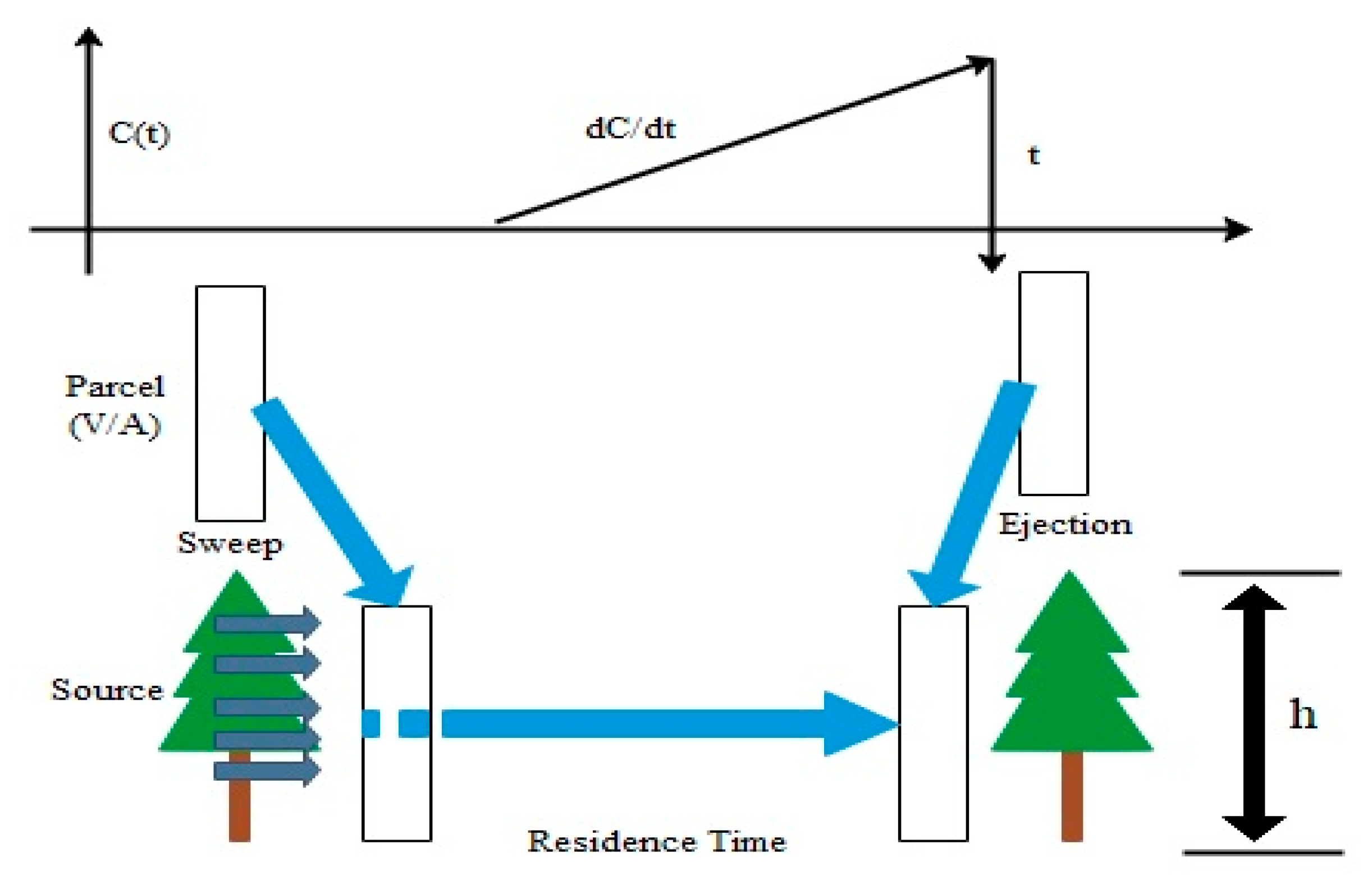
2.3. Surface Renewal (SR) Method

The SR method is based on the turbulent exchange of the sensible heat between the plant canopy and the atmosphere, caused by the instantaneous replacement of an air parcel interacting with the surface (Figure 2). The air parcel exchanges energy between air and canopy elements; then, the parcel is detached from the surface, and a new air parcel swings in to renew the removed air. Thus, understanding the features of this turbulence mechanism is vital for correct operation and analysis of this method. The signals of air temperature display well-managed coherent structures which resemble ramp events [30,31,32]. The SR method is constructed on the investigative energy budget of the coherent structures that exist within the crop canopy [31,32]. The exchange of air parcels between the surface and atmosphere is established as ramp-like shapes in the turbulence temperature; HSR can be estimated as Equation (4):
H S R =   α H S R = α z ( ρ c p ) a τ
where α is the calibration coefficient obtained through the slope of regression between HSR (calibrated sensible heat flux) and the HSR (uncalibrated sensible heat flux); z is the measurement height (m), ρ is the specific air density (kg·m−3), cp is the specific heat capacity (J·kg−1·K−1), a is the ramp amplitude (K) and τ is the ramp period (s). The SR estimations require calibration against any independent method (i.e., EC and BR).
The calibration factor (α) is obtained as the slope of the linear regression forced through the origin, between the estimations of HSR and the HEC; the value of the calibration coefficient depends on the measurement height, canopy height and architecture, atmospheric stability, turbulence characteristics, and sensor dynamic response characteristics [9]. The structure–function analysis is calculated by Equation (5) [8]:
S n ( r ) ¯   =   1 m j k = 1 m j [ ( T k T k j ) n ]
where S denotes the structure function, n is the order of the structure function (2nd, 3rd, or 5th in this case), r is the order of function, m is the total number of data points, j is the sample lag, and Tk is the kth element in the calculated temperature data. The structure–function values are used to determine the coefficient in the following cubic polynomial expressed as Equation (6) [8]:
a 3 +   p a   +   q   =   0
where p is obtained as Equation (7) [8]:
p   =   [ 10 S 2 ( r ) S 5 ( r ) S 3 ( r ) ]
Here, q is obtained as Equation (8) [8]:
q   =   10 S 3 ( r )
These equations can be solved analytically to obtain the ramp amplitude. The ramp period is calculated from the ramp amplitude, time lag, and third-order structure function using Equation (9) [8]:
τ   =   a 3 ( r ) S 3 ( r )
The shortened energy closure was used for the estimation of LE above the plant canopy using HSR and the remaining parameters, including Rn and G, using Equation (10) [8]:
L E S R =   R n     G     H S R
The performance of the SR method was analyzed by linear regression analysis against the EC system with statistical errors including root mean square error (RMSE), the slope of regression, intercept, coefficient of determination, and relative error (RE), which indicate the performance of the SR method for estimating H and LE. The SR method overcomes the issues related to the fetch, leveling, orientation, and instrument placement, which can overcome the potential uncertainties in the EC system [33,34,35,36,37].

3. Results and Discussion

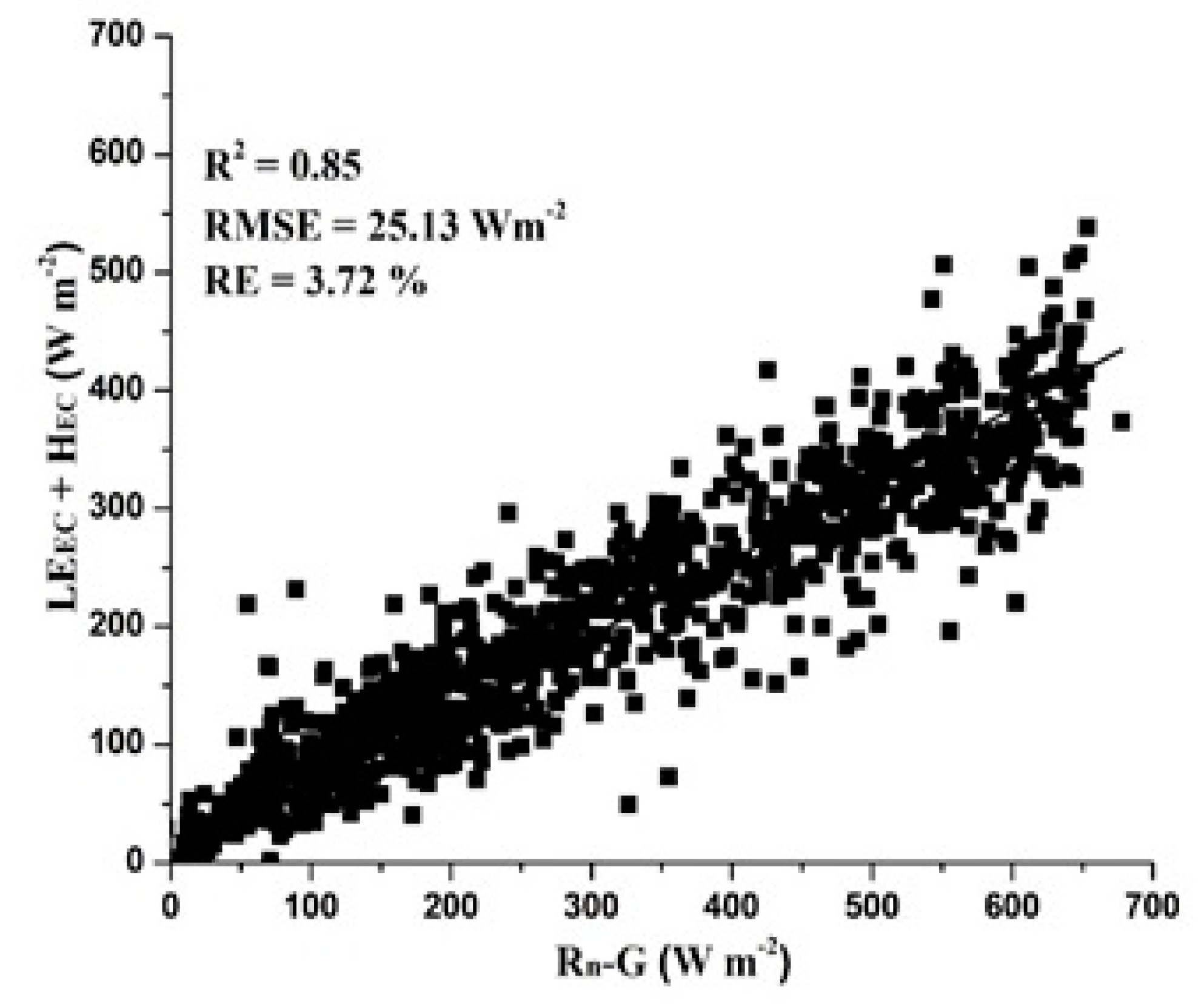
3.1. Energy Balance Closure

The energy balance closure is a typical method for evaluating the reliability of the EC system’s measurements. A half-hourly linear regression analysis was performed between the available energy fluxes (RnG) and the turbulent fluxes (LE + H) measured from the EC system (Figure 3).
In this study, measurements of the EC system were used to evaluate the performance of the SR method. Although the shortage of energy balance was within the accepted range, the estimation of LE using the SR method was based on the energy balance Equation (11):
LEEC + HEC = 0.64 (RnG)
The overall results showed that both fluxes were in good agreement, with relatively high R2 = 0.85, a slope of regression of 0.64, and statistical errors RMSE and RE of 25.13 W·m−2 and 3.72%, respectively. The energy balance slope was within the acceptable range related to the EC system application in the literature [38,39]. Hence, measurements of the EC system including the sensible heat flux and latent heat flux were used to calibrate the performance of the surface renewal method in this study.
The coherent movements of the fluxes cannot be justified by either the surface renewal or the eddy covariance method, and their role in the post-field data processing involving both of these methods remains unknown. However, this issue can play a critical role for elucidating the surface energy balance closure when the SR method is used.

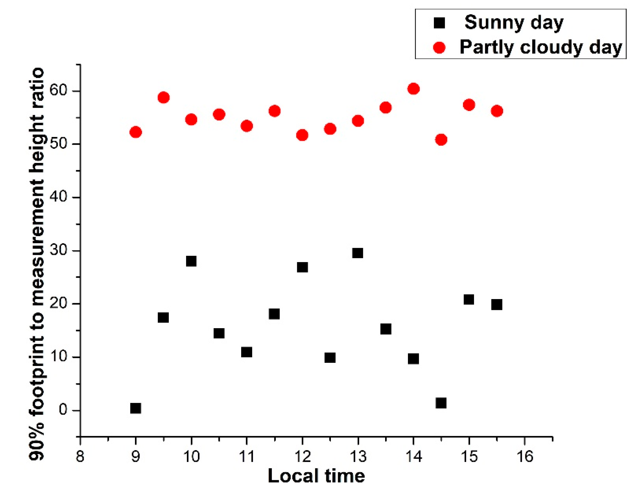
3.2. The Footprint of EC Flux Measurements

A footprint model was applied to analyze the relative contribution of the windward distance to surface fluxes measured by the EC system. The footprint model was estimated by Equations (1)–(3), which provide the ratio between 90% flux footprint and measurement height; Equation (1). The analysis was performed mostly for the daytime (unstable conditions) [27]. Two days with different climatic conditions were selected from the experimental duration: One partly cloudy (27 November 2018) and the other one (18 October 2018) a sunny day. Diurnal variations of footprint/height ratios for these two days are shown in Figure 4:
The results in Figure 4 show that the ratio during the sunny day was in the range 0–30, significantly lower than the ratio determined during the partly cloudy day which ranged between 50 and 60. This difference is presumably because during the sunny day, the surface was warmer, and the boundary layer was more unstable than during the partly cloudy day. This larger instability resulted in a shorter 90% flux footprint during the sunny than the partly cloudy day. Besides, Figure 4 shows that on both days, the ratio was smaller than the common 100:1 fetch/height ratio. This indicates that under the conditions of this experiment, most of the flux measured by the EC system originated from within the tea field under study. Hence, the EC data are reliable and can be used for the calibration of the SR method [13].

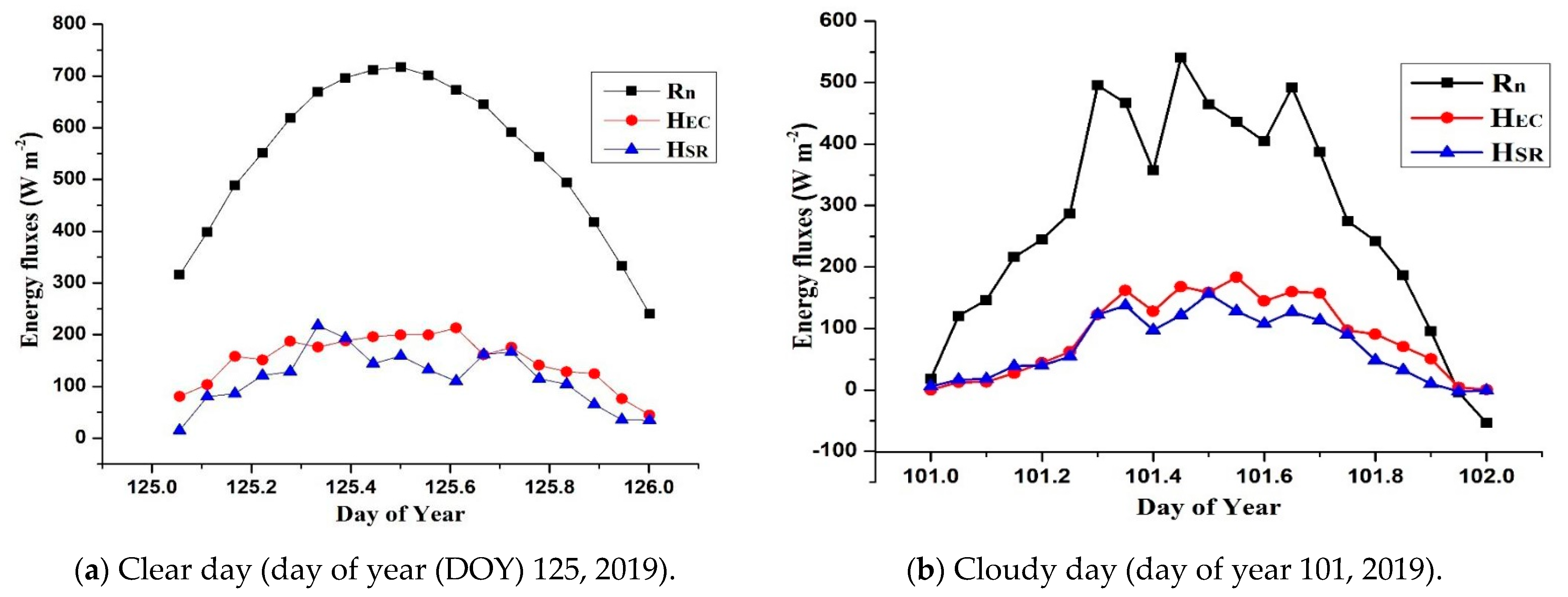
3.3. Sensible Heat Flux

The sensible heat flux was estimated using Equation (4), using high-frequency air temperature measurements of fine-wire thermocouples [34]. A linear regression analysis was performed between the half-hourly datasets of HSR and HEC under unstable conditions (Figure 5). Overall estimations of the SR method were in better agreement with the EC system with a coefficient of regression R2 = 0.80. This performance was evaluated for the time-lag of 0.5 s, keeping in view the results of previous studies using the same time-lag and frequency for the estimation of surface fluxes using the SR method and sampling frequency (~10 Hz) [10,18]. The uncalibrated HSR was corrected using the calibration coefficient of 0.68 obtained from the slope of regression between the uncalibrated and calibrated sensible heat fluxes obtained from the SR and EC systems, respectively, as shown in Table 1 for the same duration under unstable conditions. The comparison was performed to assess the performance of the SR method in tea plants.
The overall results showed good agreement between the estimations by the SR method and the EC system, with R2 = 0.80, RMSE = 27.87 W·m−2, and RE = 5.67% (Table 1). Diurnal variation of the half-hourly estimations of HSR, HEC, and Rn were observed for two randomly selected days from the experiment duration, one being a clear day (day of year 125, 2019) (Figure 6a) and one being a day with variable clouds (day of year 101, 2019) (Figure 6b).
On the clear day, the estimations were better correlated with the measurements of the EC system in the morning and in the later part of the day (evening). The overall estimation was relatively good throughout the day. On the other hand, the estimation of HSR was changing all day, corresponding to the values of Rn. In the morning, HSR was close to zero and it increased steadily with the increase in Rn; the estimation of HSR was varied with the measurement of Rn, and same trend was observed throughout the day (Figure 6a).
This showed that the air temperature fluctuations present a ramp pattern. The ramps are different for the different climatic conditions and have a direct impact on the measurements of the net radiation.

3.4. Latent Heat Flux

Latent heat flux was extracted as a residual of the energy balance closure using the estimated HSR, including the Rn and G measured separately. A linear regression analysis was performed between the half-hourly estimations of LESR and LEEC under unstable conditions, and only positive estimations of LE were compared during the analysis because only positive LE corresponds to evapotranspiration, which mainly arises under unstable conditions [40].
The HSR estimated by the SR method yielded a good estimate of the LESR using a time-lag of 0.5 s for every half-hourly dataset. The results were in good agreement with relatively high R2 = 0.93 as shown in Figure 7. The performance of the SR method for estimating LESR was evaluated using statistical tools including RMSE and RE. The best result of LESR was obtained at a height of 1.8 m above the ground, with slope of regression of 1.21. The statistical errors including RMSE and RE were obtained as 32.99 W·m−2 and 5.67%, respectively. These results represent the performance of the SR method for the estimation of LESR. The RMSE values were greater between the linear regressions of LESR vs. LEEC as compared to those of HSR vs. HEC. This was observed due to the fact that the errors were related to the measurements of Rn and G in both the SR method and the EC system (Table 2).
A diurnal comparison was made of LE with the SR estimations and the measurements by the EC system at time-lag of 0.5 s and a measurement height of 1.8 m above the ground under unstable conditions. For the comparison, two different days were selected: one with a clear sky (day of year 125, 2019) and the other with variable clouds (day of year 101, 2019). The diurnal variation of LESR and LEEC was observed with respect to the net radiation throughout the day, mainly in the daytime, usually from 8:00 to 16:00. The diurnal variation of LEEC and LESR was observed throughout the day with respect to Rn, for on a clear day, Rn was relatively high, with a maximum value of more than 700 W·m−2, and the variation of LESR and LEEC was in relatively strong agreement, mainly in the mid-day (Figure 8a).
On the other hand, the diurnal variation was in good agreement in the day with variable clouds and the estimations were directly influenced by the amount of Rn (Figure 8b). Overall, good correlation was observed throughout the day between the measurements of the EC system and the SR estimations.

4. Conclusions

The performance of the classical surface renewal method was examined in a tea plantation located in Danyang, P.R China. The conventional SR method was applied for the estimation of sensible heat flux using high-frequency air temperature measurement by fine-wire thermocouples, under unstable conditions only, and the results were compared against the measurements of the EC system. Analysis of both these methods showed that the estimated HSR corresponded well with HEC with R2 = 0.80, RMSE = 27.87 W·m−2, and RE = 9.02%, the slope of regression forced through the origin was (α = 0.68), and this slope was used for calibrating the uncalibrated sensible heat flux estimated through the SR method. The estimated LESR was in strong agreement with the latent heat flux measured by the eddy covariance system, with a relatively high coefficient of regression. Based on the results, the surface renewal method can provide simple and relatively inexpensive estimations of H and LE above tea plantations and, hence, evapotranspiration, which can help in improving the per capita production of tea plants with better irrigation application. In the future, this study can help in adopting this method for obtaining low-cost information about crop water requirements; furthermore, the SR method can be used independently in case the eddy covariance system is not available—for instance, in fields where the fetch requirement is very limited, and application of the EC system is not easy at the corner of the field. On the other hand, the SR method can be installed in a more appropriate way to obtain complete information of wind direction and other climatic factors, which can help growers to manage available irrigation resources at a relatively low cost. The results of this study were in good agreement with some previous studies performed for different crops and in different climatic conditions [5,11,17,18].

Author Contributions

Investigation, J.W. and N.A.B.; funding acquisition and supervision, Y.H.; writing—original draft, J.W. and N.A.B.; writing—review and editing, I.A.L., Q.J. and A.S. All authors have read and agreed to the published version of the manuscript.

Funding

This research was funded by the Key R&D program of Zhenjiang (NY2018007), China, and the Jiangsu Postdoctoral Science Foundations (2016M600376 and 1601032C) and Priority Academic Program Development of Jiangsu Higher Education Institutions (PAPD-2018-87).

Acknowledgments

We thank Luo Enyou for technical assistance during the experimental activities in the tea fields. We also thank the referees and editors who helped to improve the manuscript quality.

Conflicts of Interest

The authors declare no conflict of interest.

References

  1. Allen, R.; Pereira, L.; Raes, D.; Smith, M. Crop Evapotranspiration-Guidelines for Computing Crop Water Requirements-FAO Irrigation and Drainage Paper 56; Food and Agriculture Organization of the United Nations: Rome, Italy, 1998; Volume 300. [Google Scholar]
  2. Buttar, N.A.; Yongguang, H.; Shabbir, A.; Lakhiar, I.A.; Ullah, I.; Ali, A.; Aleem, M.; Yasin, M.A. Estimation of evapotranspiration using Bowen ratio method. IFAC-PapersOnLine 2018, 51, 807–810. [Google Scholar] [CrossRef]
  3. Drexler, J.Z.; Anderson, F.E.; Snyder, R.L. Evapotranspiration rates and crop coefficients for a restored marsh in the Sacramento–San Joaquin Delta, California, USA. Hydrol. Process. 2008, 22, 725–735. [Google Scholar] [CrossRef]
  4. Niaghi, A.R.; Jia, X.; Scherer, T.; Steele, D. Measurement of unirrigated turfgrass evapotranspiration rate in the red river valley. Vadose Zone J. 2019, 18, 1–11. [Google Scholar] [CrossRef] [Green Version]
  5. Castellvi, F. Combining surface renewal analysis and similarity theory: A new approach for estimating sensible heat flux. Water Resour. Res. 2004, 40, W052011–W0520120. [Google Scholar] [CrossRef] [Green Version]
  6. Savage, M.J. Estimation of evaporation using a dual-beam surface layer scintillometer and component energy balance measurements. Agric. For. Meteorol. 2009, 149, 501–517. [Google Scholar] [CrossRef]
  7. Drexler, J.Z.; Snyder, R.L.; Spano, D.; Paw, K.T. A review of models and micrometeorological methods used to estimate wetland evapotranspiration. Hydrol. Process. 2004, 18, 2071–2101. [Google Scholar] [CrossRef]
  8. Atta, V. Effect of coherent structures on structure functions of temperature in the atmospheric boundary layer. Arch. Mech. Stosow. 1977, 29, 161–171. [Google Scholar]
  9. Snyder, R.L.; Duce, P.; Paw, K.T.U. Surface renewal analysis for sensible heat flux density using structure functions. Agric. For. Meteorol. 1997, 86, 259–271. [Google Scholar]
  10. Hu, Y.; Buttar, N.A.; Tanny, J.; Snyder, R.L.; Savage, M.J.; Lakhiar, I.A. Surface Renewal Application for Estimating Evapotranspiration: A Review. Adv. Meteorol. 2018, 2018, 1–11. [Google Scholar] [CrossRef] [Green Version]
  11. Mengistu, M.G.; Savage, M.J. Surface renewal method for estimating sensible heat flux. Water SA 2010, 36, 9–18. [Google Scholar] [CrossRef]
  12. Paw, K.T.; Snyder, R.L.; Spano, D.; Su, H.B. Surface Renewal Estimates of Scalar Exchange. CA Water Plan Update 2009, 4, 1–65. [Google Scholar]
  13. Buttar, N.A.; Hu, Y.; Tanny, J.; Akram, M.W.; Shabbir, A. Fetch Effect on Flux-Variance Estimations of Sensible and Latent Heat Fluxes of Camellia sinensis. Atmosphere 2019, 10, 299. [Google Scholar] [CrossRef] [Green Version]
  14. Ullah, I.; Buttar, N.A.; Hu, Y.; Aleem, M. Height effect of air temperature measurement on sensible heat flux estimation using flux variance method. Pak. J. Agric. Sci. 2019, 56, 793–800. [Google Scholar]
  15. Castellví, F. A method for estimating the sensible heat flux in the inertial sub-layer from high-frequency air temperature and averaged gradient measurements. Agric. For. Meteorol. 2013, 180, 68–75. [Google Scholar] [CrossRef]
  16. Shabbir, A.; Mao, H.; Ullah, I.; Buttar, N.A.; Ajmal, M.; Lakhiar, I.A. Effects of drip irrigation emitter density with various irrigation levels on physiological parameters, root, yield, and quality of cherry tomato. Agronomy 2020, 10, 1685. [Google Scholar] [CrossRef]
  17. Mekhmandarov, Y.; Pirkner, M.; Achiman, O.; Tanny, J. Application of the surface renewal technique in two types of screenhouses: Sensible heat flux estimates and turbulence characteristics. Agric. For. Meteorol. 2015, 203, 229–242. [Google Scholar] [CrossRef]
  18. Poblete-Echeverría, C.; Sepúlveda-Reyes, D.; Ortega-Farías, S. Effect of height and time lag on the estimation of sensible heat flux over a drip-irrigated vineyard using the surface renewal (SR) method across distinct phenological stages. Agric. Water Manag. 2014, 141, 74–83. [Google Scholar] [CrossRef]
  19. Wyngaard, J.C.; Coté, O.R. Cospectral similarity in the atmospheric surface layer. Q. J. R. Meteorol. Soc. 1972, 98, 590–603. [Google Scholar] [CrossRef]
  20. Yongguang, H.; Chen, Z.; Pengfei, L.; Amoah, A.E.; Pingping, L. Sprinkler irrigation system for tea frost protection and the application effect. Int. J. Agric. Biol. Eng. 2016, 9, 17–23. [Google Scholar]
  21. Campbell Scientific Inc. Eddy Covariance System Doperator’s Manual, CA27 and KH20; Campbell Scientific Inc.: Logan, UT, USA, 1998. [Google Scholar]
  22. Tanny, J.; Haijun, L.; Cohen, S. Airflow characteristics, energy balance and eddy covariance measurements in a banana screenhouse. Agric. For. Meteorol. 2006, 139, 105–118. [Google Scholar] [CrossRef]
  23. Webb, E.K.; Pearman, G.I.; Leuning, R. Correction of flux measurements for density effects due to heat and water vapour transfer. Q. J. R. Meteorol. Soc. 1980, 106, 85–100. [Google Scholar] [CrossRef]
  24. Moore, C.J. Frequency response corrections for eddy correlation systems. Bound. Layer Meteorol. 1986, 37, 17–35. [Google Scholar] [CrossRef]
  25. Kljun, N.P.; Calanca, M.W.; Rotach, S.; Schmid, H.P. A simple two-dimensional parameterisation for Flux Footprint Prediction (FFP). Geosci. Model. Dev. 2015, 8, 3695–3713. [Google Scholar] [CrossRef] [Green Version]
  26. Gash, J.H.C. A note on estimating the effect of a limited fetch on micrometeorological evaporation measurements. Bound. Layer Meteorol. 1986, 35, 409–413. [Google Scholar] [CrossRef]
  27. Savage, M.J.; Everson, C.S.; Metelerkamp, B.R. Evaporation Measurement Above Vegetated Surfaces Using Micrometeorological Techniques; Water Research Commission: Pretoria, South Africa, 1997. [Google Scholar]
  28. Hsieh, C.I.; Lai, M.C.; Hsia, Y.J.; Chang, T.J. Estimation of sensible heat, water vapor, and CO2 fluxes using the flux-variance method. Int. J. Biometeorol. 2008, 52, 521–533. [Google Scholar] [CrossRef] [PubMed]
  29. Savage, M.J.; Everson, C.S.; Odhiambo, G.O.; Mengistu, M.G.; Jarmain, C. Theory and Practice of Evaporation Measurement, with Spatial Focus on SLS as an Operational Tool for the Estimation of Spatially-Averaged Evaporation; Report No. 1335/1/04; Water Research Commission: Pretoria, South Africa, 2004; p. 204. [Google Scholar]
  30. Deardorff, J.W. Observed characteristics of the outer layer. In Short Course on the Planetary Boundary Layer; American Meteorological Society: Boulder, CO, USA, 1978; p. 101. [Google Scholar]
  31. Zhao, X.; Liu, Y.; Tanaka, H.; Hiyama, T. A Comparison of Flux Variance and Surface Renewal Methods with Eddy Covariance. IEEE J. Sel. Top. Appl. Earth Obs. Remote Sens. 2010, 3, 345–350. [Google Scholar] [CrossRef]
  32. Albertson, J.D.; Parlange, M.B.; Katul, G.G.; Chu, C.R.; Stricker, H.; Tyler, S. Sensible Heat Flux from Arid Regions: A Simple Flux-Variance Method. Water Resour. Res. 1995, 31, 969–973. [Google Scholar] [CrossRef] [Green Version]
  33. Snyder, R.L.; Spano, D.; Pawu, K.T. Surface renewal analysis for sensible and latent heat flux density. Bound. Layer Meteorol. 1996, 77, 249–266. [Google Scholar] [CrossRef]
  34. Tha, P.U.K.; Jie, Q.; Hong-Bing, S.; Tomonori, W.; Yves, B. Surface renewal analysis: A new method to obtain scalar fluxes. Agric. For. Meteorol. 1995, 74, 119–137. [Google Scholar]
  35. Spano, D.; Snyder, R.L.; Duce, P.; Paw, K.T. Estimating sensible and latent heat flux densities from grapevine canopies using surface renewal. Agric. For. Meteorol. 2000, 104, 171–183. [Google Scholar] [CrossRef]
  36. Anandakumar, K. Sensible heat flux over a wheat canopy: Optical scintillometer measurements and surface renewal analysis estimations. Agric. For. Meteorol. 1999, 96, 145–156. [Google Scholar] [CrossRef]
  37. Castellví, F.; Snyder, R.L.; Baldocchi, D.D. Surface energy-balance closure over rangeland grass using the eddy covariance method and surface renewal analysis. Agric. For. Meteorol. 2008, 148, 1147–1160. [Google Scholar] [CrossRef]
  38. Aubinet, M.; Vesala, T.; Papale, D.; Kb, D.P.D.F.; William, J.M.; Loescher, H.W.; Luo, H.; Rebmann, C.; Kolle, O.; Heinesch, B.; et al. Eddy Covariance: A Practical Guide to Measurement and Data Analysis; Springer Science & Business Media: Dordrecht, The Netherlands, 2012. [Google Scholar]
  39. Wilson, K.; Goldstein, A.; Falge, E.; Aubinet, M.; Baldocchi, D.; Berbigier, P.; Bernhofer, C.; Ceulemans, R.; Dolman, H.; Field, C.; et al. Energy balance closure at FLUXNET sites. Agric. For. Meteorol. 2002, 113, 223–243. [Google Scholar] [CrossRef] [Green Version]
  40. Allen, R.G. Using the FAO-56 dual crop coefficient method over an irrigated region as part of an evapotranspiration intercomparison study. J. Hydrol. 2000, 229, 27–41. [Google Scholar] [CrossRef]
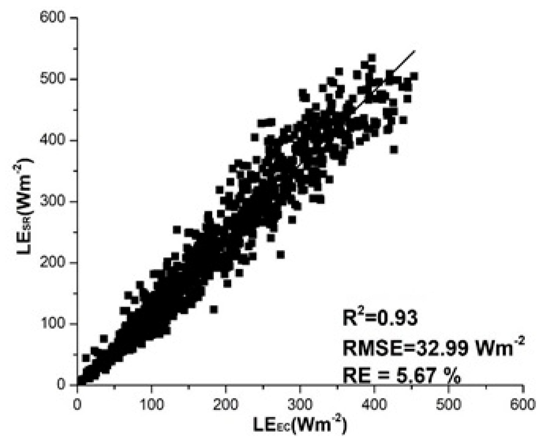
Figure 1. A map representing the location of the study area and the eddy covariance (EC) system installed at study site.
Agronomy 11 00179 g001
Figure 2. The concept of the surface renewal theory.
Agronomy 11 00179 g002
Figure 3. Half-hourly regression analysis between (RnG) and (LEEC + HEC).
Agronomy 11 00179 g003
Figure 4. Variation of half-hourly 90% footprint measurement height ratio of two different days [23].
Agronomy 11 00179 g004
Figure 5. Half-hourly regression analysis between HSR and HEC.
Agronomy 11 00179 g005
Figure 6. Diurnal variation of the half-hourly HSR, HEC, and Rn (a,b).
Agronomy 11 00179 g006
Figure 7. Half-hourly estimated LESR vs. LEEC under unstable conditions.
Agronomy 11 00179 g007
Figure 8. Variation of the Rn, LEEC, and LESR.
Agronomy 11 00179 g008
Table 1. The regression statistics between the half-hourly dataset.
Fluxesz
(m)
Time-Lag
(s)
Slope
(α)
R2RMSE
(W·m−2)
RE
(%)
HSR vs. HEC1.80.50.680.8027.879.02
LESR vs. LEEC1.80.51.210.9332.995.67
(RnG) vs. (LE + H)2.30.50.640.8525.133.72
Table 2. Experiment instruments and installation.
ObservationsNotationUnitInstallation Height (m)Instruments
3D wind velocity, sonic temperatureu, v, w, Tsm·s−1
°C
2.3CSAT3, Sonic anemometer, Camp-bell Scientific, Logan, Utah, USA
H2O and CO2 concentrations-µmol·m−32.3EC150, Campbell Scientific, Logan, Utah, USA
Soil temperatureTsoil°C0.02–0.06 (Depth)TCAV-L, Campbell Scientific, Logan, Utah, USA
Air temperature for SR analysisTa°C1.8Fine-wire thermocouple, COCO-002, Omega, Eng., UK
Relative humidityRH%2.1HC2S3-L, Campbell Scientific, Logan, Utah, USA
Soil heat fluxGW·m−20.08HFP01, Hukse flux plate sensor
Net radiationRnW·m−22.3CNR4-L, KIPP and ZENON
Liquid precipitation-mm2.1TE525MM, Campbell Scientific Inc., Logan, Utah, USA
Soil water contentϴvm3·m30.04 (Depth)CS655, Campbell Scientific Inc., Logan, Utah, USA
DataloggerCR3000 Campbell Scientific Inc., Logan, Utah, USA.
Publisher’s Note: MDPI stays neutral with regard to jurisdictional claims in published maps and institutional affiliations.

