A Compact Weighing Lysimeter to Estimate the Water Infiltration Rate in Agricultural Soils

 , , ,
, , ,  ,
,  and
and
Abstract
:1. Introduction
2. Materials and Methods
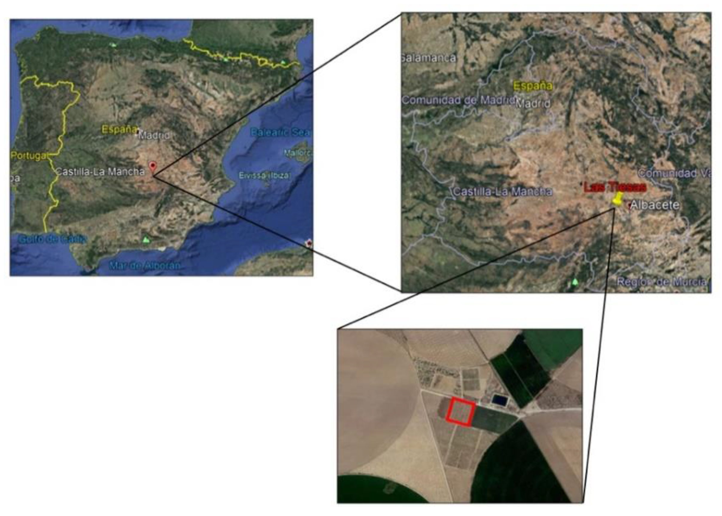
2.1. Study Area
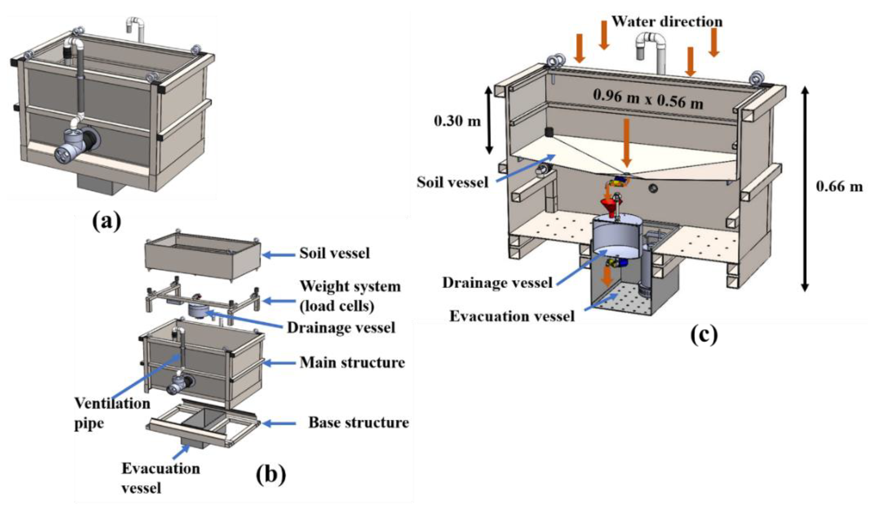
2.2. Materials
2.3. Flow Calculation
2.4. Calculation of the Infiltration Rate of Water into the Soil
2.5. Estimation of Soil Moisture Content
2.6. Validation
2.7. Model Calibrations
3. Results and Discussion
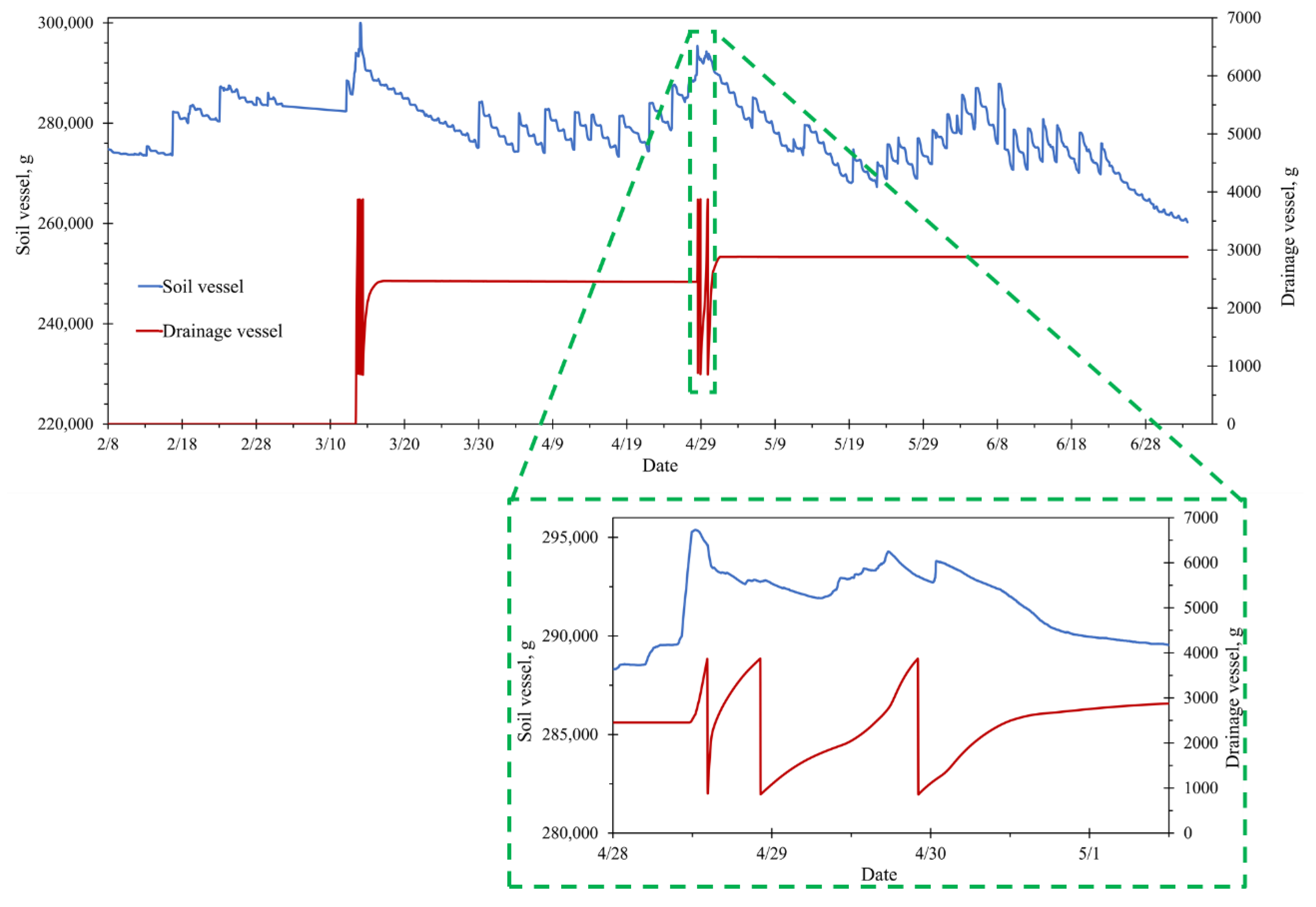
3.1. Estimation of Rain Inflow
3.2. Estimation of Soil Moisture Content
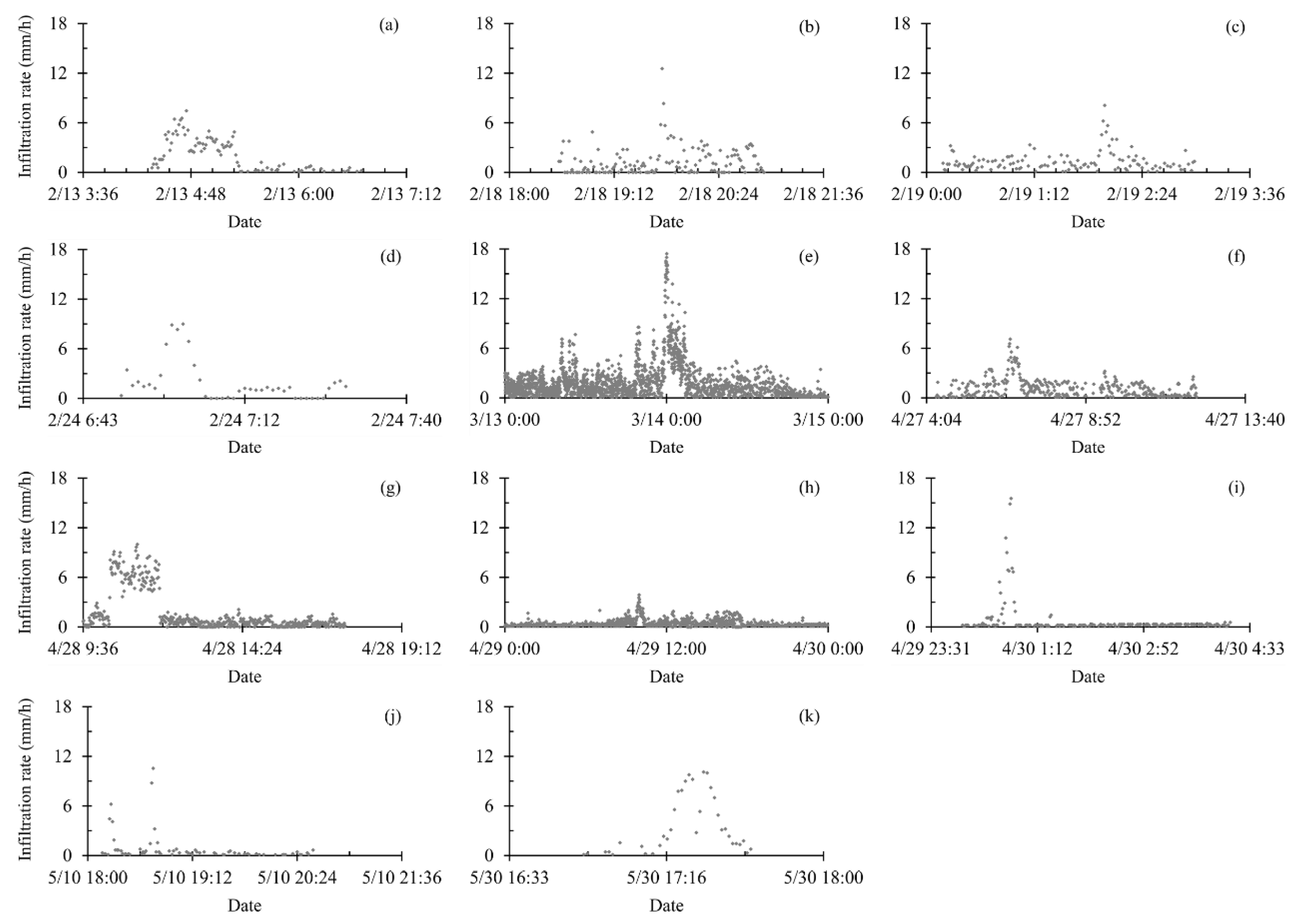
3.3. Water Infiltration Rate
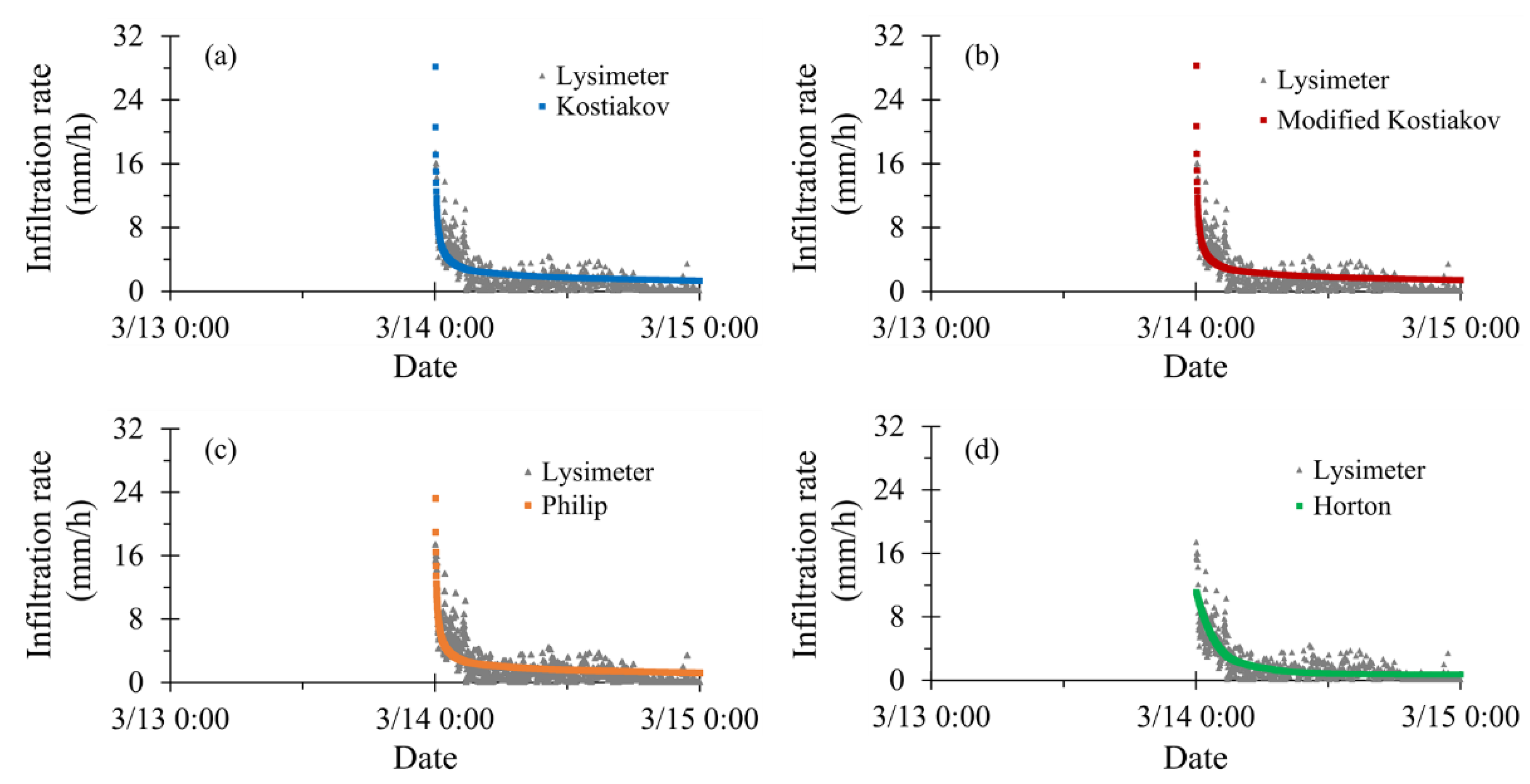
3.4. Model Calibrations
4. Conclusions
Author Contributions
Funding
Institutional Review Board Statement
Informed Consent Statement
Data Availability Statement
Acknowledgments
Conflicts of Interest
References
- Struthers, I.; Hinz, C.; Sivapalan, M.; Deutschmann, G.; Beese, F.; Meissner, R. Modelling the water balance of a free-draining lysimeter using the downward approach. Hydrol. Process. 2003, 17, 2151–2169. [Google Scholar] [CrossRef]
- Wegehenkel, M.; Zhang, Y.; Zenker, T.; Diestel, H.; Zhang, Y. The use of lysimeter data for the test of two soil-water balance models: A case study. J. Plant Nutr. Soil Sci. 2008, 171, 762–776. [Google Scholar] [CrossRef]
- Feltrin, R.M.; de Paiva, J.B.D.; de Paiva, E.M.C.D.; Beling, F.A. Lysimeter soil water balance evaluation for an experiment developed in the Southern Brazilian Atlantic Forest region. Hydrol. Process. 2011, 25, 2321–2328. [Google Scholar] [CrossRef]
- Kirkham, M. Water Movement in Saturated Soil. Princ. Soil Plant. Water Relat. 2014, 87–101. [Google Scholar] [CrossRef]
- Mendes, W.R.; de Araújo, F.M.U.; Dutta, R.; Heeren, D.M. Fuzzy control system for variable rate irrigation using remote sensing. Expert Syst. Appl. 2019, 124, 13–24. [Google Scholar] [CrossRef]
- Ali, M.H. Fundamentals of Irrigation and On-farm Water Management: Volume 1; Springer Science and Business Media LLC: Berlin/Heidelberg, Germany, 2010. [Google Scholar]
- Herrada, M.A.; Gutiérrez-Martin, A.; Montanero, J.M. Modeling infiltration rates in a saturated/unsaturated soil under the free draining condition. J. Hydrol. 2014, 515, 10–15. [Google Scholar] [CrossRef]
- Mattar, M.A.; Alazba, A.A.; El-Abedin, T.K. Forecasting furrow irrigation infiltration using artificial neural networks. Agric. Water Manag. 2015, 148, 63–71. [Google Scholar] [CrossRef]
- Yuan, J.; Feng, W.; Jang, X.; Wang, J. Saline-alkali migration in soda saline soil based on sub-soiling technology. Desalin. Water Treat. 2019, 149, 352–362. [Google Scholar] [CrossRef] [Green Version]
- Duchaufour, P. Manual de Edafología; Masson S.A.: Barcelona, Spain, 1987; ISBN 9788431104191. [Google Scholar]
- Plaster, E.J. Soil Science & Management; Editorial Paraninfo: Madrid, Spain, 2000; ISBN 84-283-2643-6. [Google Scholar]
- Wang, K.; Yang, X.; Liu, X.; Liu, C. A simple analytical infiltration model for short-duration rainfall. J. Hydrol. 2017, 555, 141–154. [Google Scholar] [CrossRef]
- Villalobos, F.J.; Mateos, L.; Orgaz, F.; Fereres, E. Fitotecnia Bases y Tecnologías de La Producción Agrícola; Mundi-Pren: Madrid, Spain, 2002; ISBN 9788484760498. [Google Scholar]
- Martín-Benito, J.M. El Riego Por Aspersión; Universidad de Castilla La Mancha: Ciudad Real, Spain, 1991. [Google Scholar]
- Harper, R.; McKissock, I.; Gilkes, R.; Carter, D.; Blackwell, P. A multivariate framework for interpreting the effects of soil properties, soil management and landuse on water repellency. J. Hydrol. 2000, 232, 371–383. [Google Scholar] [CrossRef]
- Richards, L.A. Capillary Conduction of Liquids Through Porous Mediumus. Physics 1931, 1, 318–333. [Google Scholar] [CrossRef]
- Horton, R.E. An Approach Toward a Physical Interpretation of Infiltration—Capacity 1. Soil Sci. Soc. Am. J. 1941, 5, 399–417. [Google Scholar] [CrossRef]
- Mahmood, S.; Latif, M. A Simple Procedure for Simulating Surge Infiltration Using First-Surge Infiltrometer Data. Irrig. Drain. 2005, 54, 407–416. [Google Scholar] [CrossRef]
- Teófilo-Salvador, E.; Morales-Reyes, G.P. Propuesta del modelo físico del infiltrómetro de cilindros concéntricos rediseñado multifuncional (ICCRM). Tecnol. Cienc. Agua 2018, 9, 103–131. [Google Scholar] [CrossRef]
- Arriaga, F.J.; Kornecki, T.S.; Balkcom, K.S.; Raper, R.L. A method for automating data collection from a double-ring infiltrometer under falling head conditions. Soil Use Manag. 2009, 26, 61–67. [Google Scholar] [CrossRef]
- Fatehnia, M.; Paran, S.; Kish, S.; Tawfiq, K. Automating double ring infiltrometer with an Arduino microcontroller. Geoderma 2016, 262, 133–139. [Google Scholar] [CrossRef]
- Groh, J.; Vanderborght, J.; Pütz, T.; Vereecken, H. How to Control the Lysimeter Bottom Boundary to Investigate the Effect of Climate Change on Soil Processes? Vadose Zone J. 2016, 15, 1–15. [Google Scholar] [CrossRef] [Green Version]
- Lepore, B.J.; Norman, J.M.; Lowery, B.; Brye, K.R. Soil Compaction above Long-Term Lysimeter Installations. Soil Sci. Soc. Am. J. 2011, 75, 30–34. [Google Scholar] [CrossRef]
- Masarik, K.C.; Norman, J.M.; Mason, R.E.; Baker, J.M. Improvements to Measuring Water Flux in the Vadose Zone. J. Environ. Qual. 2004, 33, 1152–1158. [Google Scholar] [CrossRef]
- Jiménez-Buendía, M.; Ruiz-Peñalver, L.; Vera-Repullo, J.; Intrigliolo-Molina, D.; Molina-Martínez, J. Development and assessment of a network of water meters and rain gauges for determining the water balance. New SCADA monitoring software. Agric. Water Manag. 2015, 151, 93–102. [Google Scholar] [CrossRef]
- Ruiz-Peñalver, L.; Vera-Repullo, J.; Jiménez-Buendía, M.; Guzman, I.; Molina-Martínez, J. Development of an innovative low cost weighing lysimeter for potted plants: Application in lysimetric stations. Agric. Water Manag. 2015, 151, 103–113. [Google Scholar] [CrossRef]
- Haselow, L.; Meissner, R.; Rupp, H.; Miegel, K. Evaluation of precipitation measurements methods under field conditions during a summer season: A comparison of the standard rain gauge with a weighable lysimeter and a piezoelectric precipitation sensor. J. Hydrol. 2019, 575, 537–543. [Google Scholar] [CrossRef]
- Meissner, R.; Seeger, J.; Rupp, H.; Seyfarth, M.; Borg, H. Measurement of dew, fog, and rime with a high-precision gravitation lysimeter. J. Plant. Nutr. Soil Sci. 2007, 170, 335–344. [Google Scholar] [CrossRef]
- Schrader, F.; Durner, W.; Fank, J.; Gebler, S.; Pütz, T.; Hannes, M.; Wollschläger, U. Estimating Precipitation and Actual Evapotranspiration from Precision Lysimeter Measurements. Procedia Env. Sci. 2013, 19, 543–552. [Google Scholar] [CrossRef] [Green Version]
- Valtanen, M.; Sillanpää, N.; Setälä, H. A large-scale lysimeter study of stormwater biofiltration under cold climatic conditions. Ecol. Eng. 2017, 100, 89–98. [Google Scholar] [CrossRef]
- Marek, G.; Gowda, P.; Marek, T.; Auvermann, B.; Evett, S.; Colaizzi, P.; Brauer, D. Estimating preseason irrigation losses by characterizing evaporation of effective precipitation under bare soil conditions using large weighing lysimeters. Agric. Water Manag. 2016, 169, 115–128. [Google Scholar] [CrossRef] [Green Version]
- Hannes, M.; Wollschläger, U.; Schrader, F.; Durner, W.; Gebler, S.; Pütz, T.; Fank, J.; Von Unold, G.; Vogel, H.-J. High-resolution estimation of the water balance components from high-precision lysimeters. Hydrol. Earth Syst. Sci. Discuss. 2015, 12, 569–608. [Google Scholar] [CrossRef] [Green Version]
- López-Urrea, R.; Montoro, A.; Mañas, F.; López-Fuster, P.; Fereres, E. Evapotranspiration and crop coefficients from lysimeter measurements of mature ‘Tempranillo’ wine grapes. Agric. Water Manag. 2012, 112, 13–20. [Google Scholar] [CrossRef]
- Luo, Y.; Sophocleous, M. Seasonal groundwater contribution to crop-water use assessed with lysimeter observations and model simulations. J. Hydrol. 2010, 389, 325–335. [Google Scholar] [CrossRef]
- Kelleners, T.J.; Soppe, R.; Ayars, J.E.; Šimunek, J.; Skaggs, T.H. Inverse Analysis of Upward Water Flow in a Groundwater Table Lysimeter. Vadose Zone J. 2005, 4, 558–572. [Google Scholar] [CrossRef] [Green Version]
- Dijkema, J.; Koonce, J.; Shillito, R.; Ghezzehei, T.; Berli, M.; van der Ploeg, M.; Van Genuchten, M. Water Distribution in an Arid Zone Soil: Numerical Analysis of Data from a Large Weighing Lysimeter. Vadose Zone J. 2017, 17, 170035. [Google Scholar] [CrossRef] [Green Version]
- Germann, P.; Prasuhn, V. Viscous Flow Approach to Rapid Infiltration and Drainage in a Weighing Lysimeter. Vadose Zone J. 2017, 17, 170020. [Google Scholar] [CrossRef] [Green Version]
- Schwaerzel, K.; Bohl, H.P. An easily installable groundwater lysimeter to determine water balance components and hydraulic properties of peat soils. Hydrol. Earth Syst. Sci. 2003, 7, 23–32. [Google Scholar] [CrossRef]
- Google Earth. Available online: https://earth.google.com/web/ (accessed on 14 March 2020).
- Conklin, H.E. Soil Survey Manual. J. Farm. Econ. 1952, 34, 145. [Google Scholar] [CrossRef]
- Automatic Weather Station Network. Criteria for the Localization of Sites and Installation of Sensor. Adquisition Characteristics and Sampling. In UNE 500520-2002; Spanish Standardization (UNE, Spanish Acronyms). Elaborated by the Technical Committee AEN/CTN GET5 Meteorological Records Whose Secretariat Is Provided by AENOR-PUERTOS DEL ESTADO; Spanish Association for Standardization and Certification (AENOR, Spanish Acronyms): Madrid, Spain, 2002. [Google Scholar]
- Nicolás-Cuevas, J.A.; Parras-Burgos, D.; Soler-Méndez, M.; Ruiz-Canales, A.; Molina-Martínez, J.M. Removable Weighing Lysimeter for Use in Horticultural Crops. Appl. Sci. 2020, 10, 4865. [Google Scholar] [CrossRef]
- Peters, A.; Nehls, T.; Schonsky, H.; Wessolek, G. Separating precipitation and evapotranspiration from noise—A new filter routine for high-resolution lysimeter data. Hydrol. Earth Syst. Sci. 2014, 18, 1189–1198. [Google Scholar] [CrossRef] [Green Version]
- Gebler, S.; Hendricks-Franssen, H.-J.; Putz, T.; Post, H.; Schmidt, M.; Vereecken, H. Actual evapotranspiration and precipitation measured by lysimeters: A comparison with eddy covariance and tipping bucket. Hydrol. Earth Syst. Sci. 2015, 19, 2145–2161. [Google Scholar] [CrossRef] [Green Version]
- Wang, N.; Chu, X. Revised Horton model for event and continuous simulations of infiltration. J. Hydrol. 2020, 589, 125215. [Google Scholar] [CrossRef]
- Hartley, D.M. Interpretation of Kostiakov Infiltration Parameters for Borders. J. Irrig. Drain. Eng. 1992, 118, 156–165. [Google Scholar] [CrossRef]
- Lewis, M.R. The rate of infiltration of water in irrigation-practice. Trans. Am. Geophys. Union 1937, 18, 361–368. [Google Scholar] [CrossRef]
- Fok, Y. Derivation of Lewis-Kostiakov Intake Equation. J. Irrig. Drain. Eng. 1986, 112, 164–171. [Google Scholar] [CrossRef]
- Haverkamp, R.; Kutilek, M.; Parlange, J.Y.; Rendon, L.; Krejca, M. Infiltration under Ponded Conditions: 2. Infiltration Equations Tested for Parameters Time-Dependece and Predictive Use1. Soil Sci. 1988, 145, 317–329. [Google Scholar] [CrossRef]
- Philip, J.R. The Theory of Infiltration: 4. Sorptivity and Algebraic Infiltration Equation. Soil Sci. 1957, 84, 257–264. [Google Scholar] [CrossRef]
- Smerdon, E.T.; Blair, A.W.; Reddell, D.L. Infiltration from Irrigation Advance Data. I: Theory. J. Irrig. Drain. Eng. 1988, 114, 4–17. [Google Scholar] [CrossRef]
- Haghiabi, A.H.; Abedi-Koupai, J.; Heidarpour, M.; Mohammadzadeh-Habili, J. A New Method for Estimating the Parameters of Kostikov and Modified Kostiakov Infiltration Equations. World Appl. Sci. J. 2011, 15, 129–135. [Google Scholar]
- Strelkoff, T.S.; Clemmens, A.J.; Bautista, E. Field Properties in Surface Irrigation Management and Design. J. Irrig. Drain. Eng. 2009, 135, 525–536. [Google Scholar] [CrossRef] [Green Version]
- Furman, A.; Warrick, A.W.; Zerihun, D.; Sanchez, C.A. Modified Kostiakov Infiltration Function: Accounting for Initial and Boundary Conditions. J. Irrig. Drain. Eng. 2006, 132, 587–596. [Google Scholar] [CrossRef]
- Wackerly, D.D.; Mendenhall, W.; Schaeaffer, R.L. Mathematical Statics with Applications, 7th ed.; Ceneage Learning: Boston, MA, USA, 2010. [Google Scholar]
- Belmonte, A.M.C.; García, J.S.; García, M.J.L. The effect of observation timescales on the characterisation of extreme Mediterranean precipitation. Adv. Geosci. 2010, 26, 61–64. [Google Scholar] [CrossRef] [Green Version]
- Assi, A.; Blake, J.; Mohtar, R.H.; Braudeau, E. Soil aggregates structure-based approach for quantifying the field capacity, permanent wilting point and available water capacity. Irrig. Sci. 2019, 37, 511–522. [Google Scholar] [CrossRef]
- Allen, R.G.; Pereira, L.S.; Raes, D.; Smith, M. Crop Evapotranspiration-Guidelines for Computing Crop Water Requirements; FAO Irrigation and Drainage Paper 56; FAO Rome: Roma, Italy, 1998; Volume 300, p. d05109. [Google Scholar]
- Porta-Casanellas, J.; Lopez-Acevedo, R.M. Agenda de Campo de Suelos. Información de Suelos Para La Agricultura y El Medio Ambiente; Ediciones Mundi-Prensa: Madrid, Spain, 2005. [Google Scholar]
- USDA (United State Department of Agricultura); NRCS (Natural Resources Conservation Service); ARS (Agricultural Research Service); SQI (Soil Quality Institute). Soil Quality Test Kit Guide; U.S. Department of Agriculture: Washington, DC, USA, 2001.
- Evanylo, G.; McGuinn, R. Agricultural Management Practices and Soil Quality; Virginia Polytechnic Institute and State University, College of Agriculture and Life Sciences: Blacksburg, VA, USA, 2000; Volume 5. [Google Scholar]
- Cui, Z.; Wu, G.-L.; Huang, Z.; Liu, Y. Fine roots determine soil infiltration potential than soil water content in semi-arid grassland soils. J. Hydrol. 2019, 578, 124023. [Google Scholar] [CrossRef]
- Liu, Y.; Cui, Z.; Huang, Z.; López-Vicente, M.; Wu, G.-L. Influence of soil moisture and plant roots on the soil infiltration capacity at different stages in arid grasslands of China. Catena 2019, 182, 104147. [Google Scholar] [CrossRef]
- Li, Y.; Ren, X.; Hill, R.; Malone, R.; Zhao, Y.; Ying, Z.; Malonew, R. Characteristics of Water Infiltration in Layered Water-Repellent Soils. Pedosphere 2018, 28, 775–792. [Google Scholar] [CrossRef]
- Maldonado, T. Manual de Riego Parcelario. Available online: http://www.fao.org/tempref/GI/Reserved/FTP_FaoRlc/old/prior/recnat/pdf/MR_cap1.PDF (accessed on 30 January 2020).
- Rodríguez-Vásquez, A.F.; Aristizábal-Castillo, A.M.; Camacho-Tamayo, J.H. Variabilidad Espacial de los Modelos de Infiltración de Philip y Kostiakov en un Suelo Ândico. Eng. Agríc. 2008, 12, 64–75. [Google Scholar] [CrossRef] [Green Version]
- Mirzaee, S.; Zolfaghari, A.A.; Gorji, M.; Dyck, M.; Dashtaki, S.G. Evaluation of infiltration models with different numbers of fitting parameters in different soil texture classes. Arch. Agron. Soil Sci. 2013, 60, 681–693. [Google Scholar] [CrossRef]


| Date | Rain Registered per Day | |
|---|---|---|
| Weighing Lysimeter | Weather Station ITAP | |
| (mm) | (mm) | |
| 02/13 | 3.55 | 3.60 |
| 02/18 | 3.16 | 3.30 |
| 02/19 | 2.76 | 2.90 |
| 02/24 | 1.30 | 1.00 |
| 03/13 | 36.77 | 26.70 |
| 03/14 | 28.53 | 22.30 |
| 04/27 | 7.04 | 6.40 |
| 04/28 | 7.06 | 5.90 |
| 04/29 | 8.16 | 8.30 |
| 04/30 | 2.44 | 1.6 |
| 05/10 | 1.01 | 1.10 |
| 05/30 | 2.11 | 1.60 |
| Date | ||||
|---|---|---|---|---|
| 03/13 | 0.00 | 36.77 | 14.04 | 0.00 |
| 03/14 | 0.00 | 28.53 | 29.57 | 5.41 |
| 04/28 | 10.62 | 5.90 | 8.65 | 0.00 |
| 04/29 | 0.00 | 8.30 | 5.65 | 0.65 |
| 04/30 | 0.00 | 1.60 | 3.05 | 4.94 |
| Method of Estimation and Authors | ||
|---|---|---|
| 0.33 | Weighing Lysimeter | |
| 0.35 | Laboratory | |
| 0.22–0.36 | FAO | [58] |
| 0.30–0.31 | Pedostructure | [57] |
| 0.244 | Gravimetric | [59] |
Publisher’s Note: MDPI stays neutral with regard to jurisdictional claims in published maps and institutional affiliations. |
© 2021 by the authors. Licensee MDPI, Basel, Switzerland. This article is an open access article distributed under the terms and conditions of the Creative Commons Attribution (CC BY) license (http://creativecommons.org/licenses/by/4.0/).
Share and Cite
Ávila-Dávila, L.; Soler-Méndez, M.; Bautista-Capetillo, C.F.; González-Trinidad, J.; Júnez-Ferreira, H.E.; Robles Rovelo, C.O.; Molina-Martínez, J.M. A Compact Weighing Lysimeter to Estimate the Water Infiltration Rate in Agricultural Soils. Agronomy 2021, 11, 180. https://0-doi-org.brum.beds.ac.uk/10.3390/agronomy11010180
Ávila-Dávila L, Soler-Méndez M, Bautista-Capetillo CF, González-Trinidad J, Júnez-Ferreira HE, Robles Rovelo CO, Molina-Martínez JM. A Compact Weighing Lysimeter to Estimate the Water Infiltration Rate in Agricultural Soils. Agronomy. 2021; 11(1):180. https://0-doi-org.brum.beds.ac.uk/10.3390/agronomy11010180
Chicago/Turabian StyleÁvila-Dávila, Laura, Manuel Soler-Méndez, Carlos Francisco Bautista-Capetillo, Julián González-Trinidad, Hugo Enrique Júnez-Ferreira, Cruz Octavio Robles Rovelo, and José Miguel Molina-Martínez. 2021. "A Compact Weighing Lysimeter to Estimate the Water Infiltration Rate in Agricultural Soils" Agronomy 11, no. 1: 180. https://0-doi-org.brum.beds.ac.uk/10.3390/agronomy11010180