Dual Crop Coefficient Approach in Vitis vinifera L. cv. Loureiro

Abstract

Vineyard irrigation management in temperate zones requires knowledge of the crop water requirements, especially in the context of climate change. The main objective of this work was to estimate the crop evapotranspiration (ET_c) of Vitis vinifera cv. Loureiro for local conditions, applying the dual crop coefficient approach. The study was carried out in a vineyard during two growing seasons (2019–2020). Three irrigation treatments, full irrigation (FI), deficit irrigation (DI), and rainfed (R), were considered. The ET_c was estimated using the SIMDualKc model, which performs the soil water balance with the dual Kc approach. This balance was performed by calculating the basal coefficients for the grapevine (K_{cb crop}) and the active soil ground cover (K_{cb gcover}), which represent the transpiration component of ET_c and the soil evaporation coefficient (K_e). The model was calibrated and validated by comparing the simulated soil water content (SWC) with the soil water content data measured with frequency domain reflectometry (FDR). A suitable adjustment between the simulated and observed SWC was obtained for the 2019 R strategy when the model was calibrated. As for the vine crop, the best fit was obtained for K_{cb full ini} = 0.33, K_{cb full mid} = 0.684, and K_{cb full end} = 0.54. In this sense, the irrigation schedule must adjust these coefficients to local conditions to achieve economically and environmentally sustainable production.

1. Introduction

The sustainability of wine production is a global strategy that includes all stages of the wine production cycle. In achieving sustainable wine production, the environmental aspects, such as efficient water use, should be considered [1]. Water is a factor that significantly influences crop yields [2], and it must be applied sustainably and efficiently [3]. This application must be efficient because, according to predictions, global water extraction will increase by 55% between 2000 and 2050 in a similar scenario to the current one [4]. In addition, predictions estimate a 20% decrease in precipitation in the Vinhos Verdes region, according to the IPCC RCP8.5 scenario [5].

To implement a sustainable strategy, it is necessary to expand the knowledge on crop evapotranspiration to support appropriate irrigation scheduling and management [5]. The estimation of crop evapotranspiration can be obtained with the single or dual crop coefficient approach (dual Kc) [6] through various field measurements techniques, for example, remote sensor data [7,8], eddy covariance [9], lysimeter [10,11], and measurements of soil water content [12,13].

The dual Kc approach estimates the actual crop evapotranspiration (ET_{c act}) through reference evapotranspiration (ET_o) and actual crop coefficient (K_{c act}). Adopting this dual Kc approach (Equation (1)), the K_{c act} results from the sum of the basal crop coefficients (K_cb), correcting through a stress coefficient (K_s) that varies between 0 (maximum stress) and 1 (no stress), with the soil evaporation (K_e) [6]. Thus, ET_{c act} is defined as follows:

$${\mathrm{ET}}_{\mathrm{c} \mathrm{act}}=\left({\mathrm{K}}_{\mathrm{s}}\times { \mathrm{K}}_{\mathrm{cb}}+{\mathrm{K}}_{\mathrm{e}}\right)\times {\mathrm{ET}}_{\mathrm{o}}={ \mathrm{K}}_{\mathrm{c} \mathrm{act}}\times {\mathrm{ET}}_{\mathrm{o}}$$

(1)

where K_s represents the stress coefficient, K_cb is the basal crop coefficient, K_e is the soil evaporation coefficient, and ET_o represents the reference evapotranspiration (mm d⁻¹).

During the active growing season, variations in the density and height of active soil ground cover are observed in the vineyards of this region. These variations are influenced by cultural operations aimed at controlling the active soil ground cover’s vegetative vigor (herbicide application or tillage operations), as well as by climatic factors [14]. The water consumption of the active soil ground cover is environmentally acceptable when considering the numerous ecosystem services provided by cover crops in vineyards [15], such as the prevention of erosion [16], the contribution to carbon (C) sequestration, the increase in total nitrogen (N) content [17], and the contributions to plant vigor and fruit quality control [18], as well as pest control [19]. However, water consumption must also be considered in crop evapotranspiration [9]. In this sense, following the dual Kc approach, the active soil ground cover represents a part of the evapotranspiration. Therefore, the total evapotranspiration results from the sum of the transpiration from active soil ground cover and vineyard with the soil evaporation [20].

The dual Kc approach for computing and partitioning crop evapotranspiration can be facilitated using index and models applications, such as the Satellite-based NDVI [21], AquaCrop model [22], and SIMDualKc model [23,24]. The SIMDualKc performs the soil water balance at the field level, using a daily timestep, based on Equation (2):

$${\mathrm{D}}_{\mathrm{i}}{=\mathrm{D}}_{\mathrm{i}-1}-{(\mathrm{P}-\mathrm{RO})}_{\mathrm{i}}-{\mathrm{I}}_{\mathrm{i}}-{\mathrm{CR}}_{\mathrm{i}}{+\mathrm{ET}}_{\mathrm{c}, \mathrm{i}}{+\mathrm{DP}}_{\mathrm{i}}$$

(2)

where D_i−1 is the depletion at the preceding day, P is the precipitation, I is the irrigation, CR is the capillary rise from a shallow water table, DP is the deep percolation out of the root zone, ETc,_i is the crop evapotranspiration (mm), and RO is the runoff, with all terms expressed in mm.

This model was validated using data from several permanent crops with active soil ground cover, namely olives [8,9] and hop [25]. The model was also validated for the culture of Vitis vinifera, where studies on cv. Albariño [20] and Godello e Mencía [26], took into account the effect of active ground cover. In these studies, the SIMDualKc model has been shown to be appropriate for adopting the dual Kc approach. In addition, to help computing and partitioning crop evapotranspiration, SIMDualKc has been used to update dual crop coefficients for many crops [27,28,29,30,31].

The present study aims to provide information on evapotranspiration and crop coefficients for Vitis vinifera cv. Loureiro in northwest Portugal. The specific objectives of this paper are: (a) to calibrate and validate the SIMDualKc model using the dual Kc approach, (b) to provide the K_cb for each growth stage of the crop, (c) to apply the dual Kc approach to different irrigation strategies and (d) to verify if cv. Loureiro cultivated without irrigation (the most practiced in the region) is cultivated under drought stress. The results obtained in this work aim to support irrigation management programs, improving the use of water in agriculture.

2. Materials and Methods

2.1. Study Area

The study was carried out in a commercial cv. Loureiro vineyard, located in Ponte de Lima, in northwest Portugal (41°40′32″ N, 8°32′6″ W, and 170 m.a.s.l.) during two growing seasons (2019 and 2020). The vineyard was planted in 2001, with a distance between rows of 3.0 m and a distance of 2.0 m between vines (1666 plant ha⁻¹). The vineyard is north–south orientated and trained to a single upward cordon. Drip irrigation was installed as the irrigation system, with one drip line per row, located at 40 cm above the ground and pressure-compensated emitters (4 L h⁻¹) separated by one meter. The climate is Atlantic, characterized by relatively high annual rainfall (above 1200 mm) and relatively mild summers [32]. The Köppen–Geiger [33] classification is Csb.

The daily meteorological data (temperature, humidity, wind speed at 2 m height, net radiation, and precipitation) were collected from the weather station (UNL Ameriflux Site, Mead NE) located in the field. The ET_o was computed with the FAO Penman–Monteith Equation (3) [6], which, for the computation of daily timesteps, takes the following form:

$${\mathrm{ET}}_{\mathrm{o}}=\frac{0.408 \Delta \left({\mathrm{R}}_{\mathrm{n} }- \mathrm{G}\right)+\mathsf{\gamma } \frac{900}{\mathrm{T}+273}{\mathrm{U}}_2\left({\mathrm{e}}_{\mathrm{a}}-{ \mathrm{e}}_{\mathrm{d}}\right)}{\Delta +\mathsf{\gamma } \left(1 - 0{.34\mathrm{U}}_2\right)}$$

(3)

where Δ represents the slope of the saturation vapor pressure-temperature relationship at the mean air temperature (kPa °C⁻¹), R_n is the net radiation at the crop surface (MJ m⁻² d⁻¹), G is the soil heat flux density (MJ m⁻² d⁻¹), γ is the psychometric constant (kPa °C⁻¹), T is the mean daily air temperature (°C), U₂ is the wind speed (m s⁻¹) at 2 m height and (e_a − e_d) represents the vapor pressure at the reference height of 2 m and deficit of air (kPa) at 2 m height.

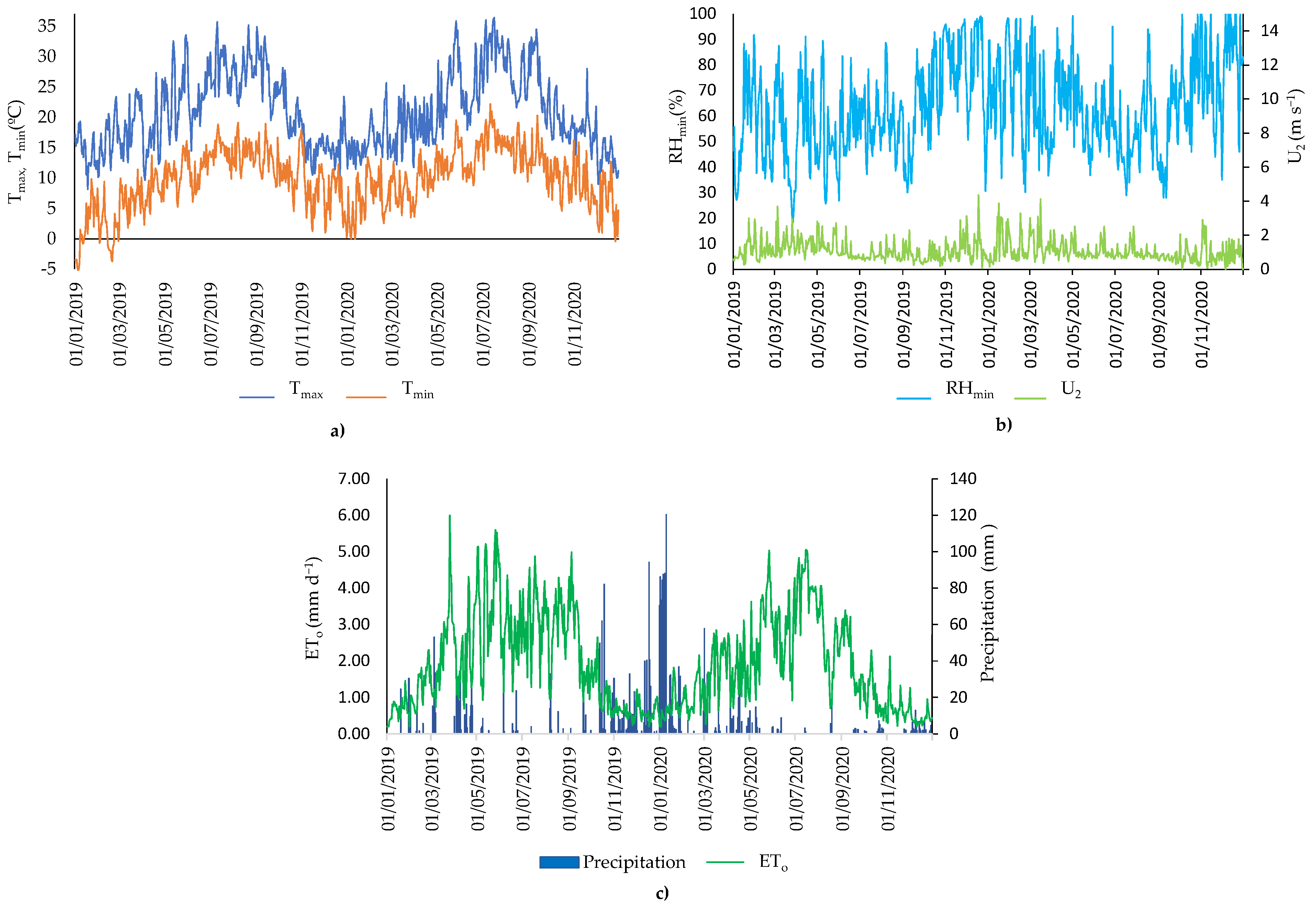
The total rainfall was 1431 and 1590 mm in 2019 and 2020, respectively. In the growing season, the rainfall was 402 mm and 321 mm for 2019 and 2020, respectively (Figure 1). The ET_o was higher in the summer, reaching 116 mm month−¹ in May 2019 and 126 mm month⁻¹ in July 2020 (Figure 1). However, its daily variability was high depending on the net radiation, temperature, and wind speed.

2.2. Climate and Soil Characterization

The climate directly and indirectly affects crop production and bioclimatic indices can be used to characterize the climate. Therefore, in this work, we used the Winkler index (WI), Huglin index (HI), Cool night index (CI), Seljaninov index (SI), and Branas index (BI), which have already been used by other authors in this region [34]. According to the climatic characterization shown in Figure 1, the growing seasons were very different with respect to the temperatures and precipitation values observed. The results of applying Equations (4) and (5) in 2019 are lower than the results for 2020 (

Table 1. List of the bioclimatic indices used for this study for both years, their corresponding mathematical definitions, and sources.

Index and Abbreviation	Equation		Source	Results
				2019	2020
Winkler index (WI)	${\displaystyle {\displaystyle \sum }_{01.04}^{30.10}}(T_{avg}-10 ℃)$	(4)	[35]	1771	2124
Huglin index (HI)	${\displaystyle {\displaystyle \sum }_{01.04}^{30.09}}\frac{(T_{avg}-10)+(T_{máx}-10)}{2}\times k$	(5)	[36]	2847	2937
Cool night index (CI)	$T_{min\mathrm{average} }\left(\mathrm{september}\right)$	(6)	[37]	13.22	13.05
Seljaninov index (SI)	$\sum (P/(\sum ((T_{avg}-10 °\mathrm{C}\left)\right)\left)\right)$	(7)	[38]	0.27	0.29
Branas index (BI)	${\displaystyle {\displaystyle \sum }_{01.04}^{31.08}}{T}_{avg}\times P_{month}$	(8)	[39]	18,654	11,677

T_máx is maximum air temperature (°C), T_min is minimum air temperature (°C), T_avg is mean air temperature (°C), k is the length of day coefficient, and P is precipitation (mm).

). Thus, it is possible to verify that, in general, lower temperatures were observed in 2019. However, according to Equation (6), the minimum temperature in September 2019 was higher than the minimum temperature recorded in the same period in 2020 (Table 1). As the precipitation values were very different (Figure 1), the results of the application indexes that relate temperatures with precipitation Equations (7) and (8) were also very different in the two years of the study. Therefore, the results of Equations (7) and (8) obtained for 2019 were different from those obtained for 2020(Table 1).

The soil was classified as eutric regosol [40], with a sandy loam texture. On average, the soil contained 70.2% sand, 20.3% silt, and 9.5% clay, with 1.95% organic matter. The total available soil water (TAW) at a depth of 0.8 m (m) was 100 mm. The TAW was calculated from the difference between the soil field capacity and the permanent wilting point using eight soil layers.

The field capacity and wilting point were obtained in the laboratory. To determine the field capacity, a pressure plate was used to apply a suction of −1/3 of the atmosphere to the saturated soil samples. With the same samples, a suction of −15 atmospheres was applied to determine the wilting point [41]. The field capacity and wilting point values were 0.251 and 0.121 cm³ cm⁻³, respectively. Capacitive probes were used to determine the field capacity value in situ in eight different soil layers up to 0.8 m, which ranged between 0.197 and 0.273 cm³ cm⁻³ for the depths of 0.1 m and 0.8 m, respectively. These values were used in the SWC simulation.

2.3. Experimental Design: Data Required to Apply SIMDualKc

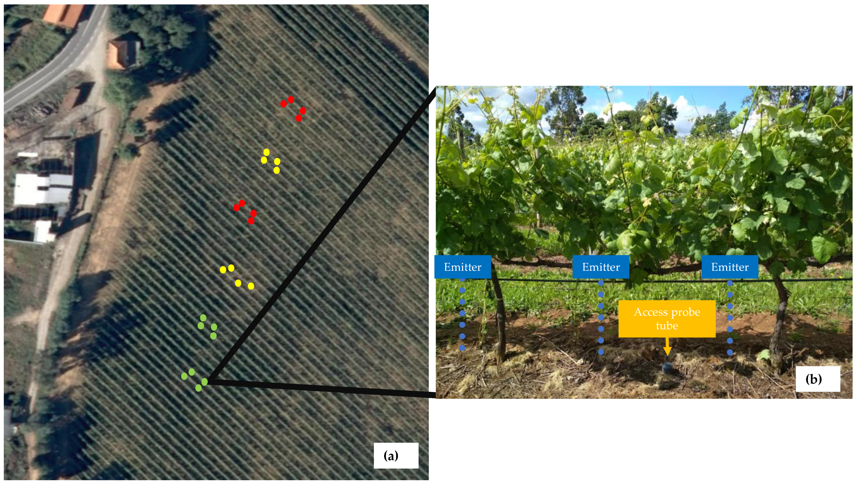
Three irrigation treatments were considered, full irrigation (defined by the vinegrower; FI), deficit irrigation (DI), and rainfed (R), which is most practiced in the region. Each treatment had two replicates (Figure 2a) with four rows; in the two central rows were installed access probes and the other two rows were used as buffers (Figure 2a). To obtain the SWC readings, 24 access probe tubes (80 cm depth) were installed in the rows (Figure 2b), distributed over the treatments (8 access probe tubes per treatment). In 2019, irrigation was implemented between DOY 142 and DOY 238 to FI treatment when the volumetric soil moisture content was 90% of field capacity and reached 69.67 mm (10 irrigation events), while for the treatment DI was implemented between DOY 204 and DOY 217 when the volumetric soil moisture content was 70% of field capacity and reached 17.33 mm (two irrigation events). In 2020, the irrigation was implemented between DOY 181 and DOY 224, when the volumetric soil moisture content was 70% of field capacity and reached 94 mm (10 irrigation events) in FI, whereas the DI reached 32 mm (6 irrigation events), FI in 2020 started later than in 2019 due to problems in the irrigation system.

Based on the successive SWC readings carried out with a capacitive probe (Diviner 2000) after the occurrence of high precipitation, the drainage depletion curve for the soil was obtained by applying the power regression method, Equation (9), defined by Liu et al. (2006) [42]:

$$SWC=a\times t^b$$

(9)

where SWC represents soil water content in mm, a is soil water storage value comprised between field capacity and saturation of the soil, b represents the velocity of drainage, and t is the time in days. The parameters a and b were defined as 287.05 and −0.056, respectively. A curve number of 60 was used to calculate the surface runoff [23,43].

Phenological evolution was performed based on the Baggiolini scale [44], which was later adapted to our FAO standard crop growth stages. Therefore, the day when the vine reached stage D (leaf emergence) corresponds to the start of the rapid growth stage [6], and the midseason stage corresponds to the period between phases: I (flowering) and phase M (veraison).

Crop heights (h) (from the soil) and the fraction of soil shaded by the crop (f_c), was determined through visual observation at solar noon and were observed throughout the active growing season. The values at the dates of the crop growth stages are presented in

Table 2. Vineyard crop growth stages, height (h), and fraction of the soil covered by the crop in the vineyard (f_c).

Crop Growth Stages	2019			2020
	Dates	H (m)	fc	Dates	H (m)	fc
Initiation	21 March	1.0	0.01	1 March	1.0	0.01
Start rapid growth	26 March	1.4	0.05	28 March	1.2	0.05
Start midseason	6 June	2.0	0.30	22 June	2.0	0.30
Start maturity	2 September	2.4	0.40	20 August	2.4	0.40
Harvesting	23 September	2.4	0.40	9 September	2.4	0.40

.

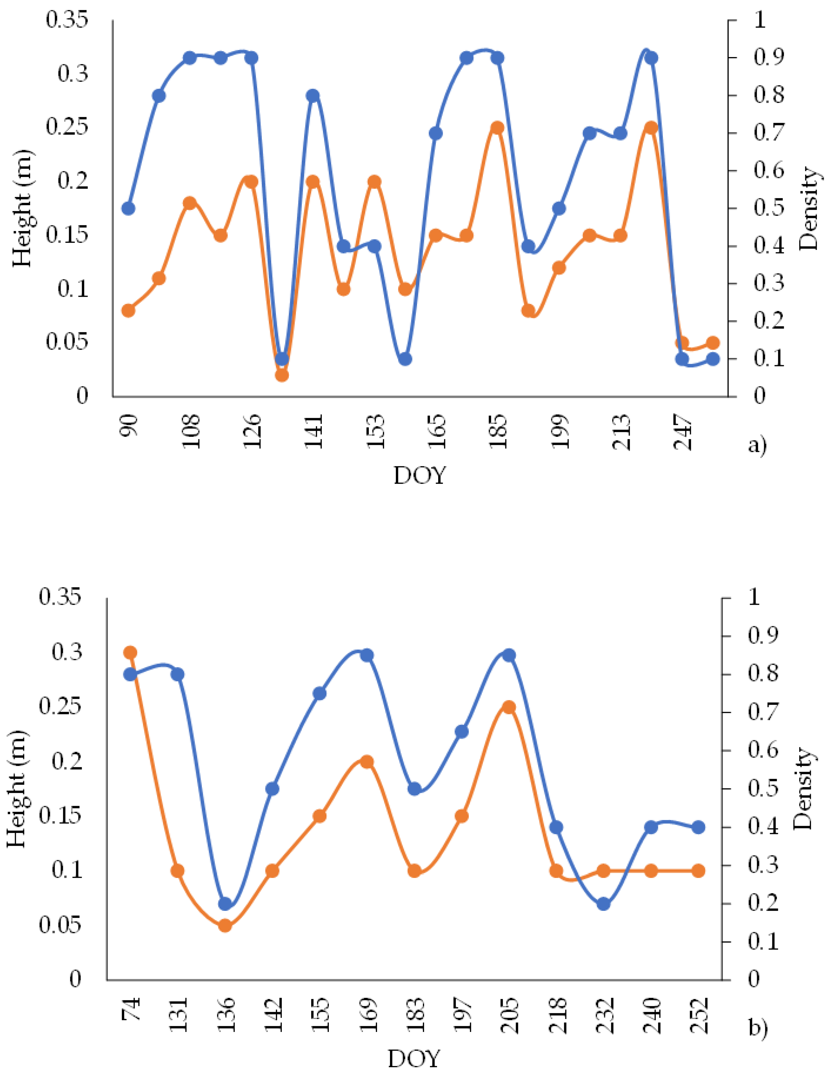
The active ground cover was composed of spontaneous species. In 2019, the density of the active coverage (performed by observation) varied between 10% and 90%, with height varied between 0.02 and 0.25 m between the rows and no active coverage in the row (

Table A1. Density and height of the green active ground cover for the 2 experimental seasons (2019–2020). Row and inter-row data.

Year	DOY	CC_dens_Row	CC_dens_InterRow	CC_Height_Row (m)	CC_Height_intRow (m)
2019	80	0	0.50	0	0.05
	91	0	0.50	0	0.08
	106	0	0.80	0	0.11
	109	0	0.90	0	0.18
	112	0	0.90	0	0.15
	127	0	0.90	0	0.20
	133	0	0.10	0	0.02
	142	0	0.80	0	0.20
	148	0	0.40	0	0.10
	154	0	0.40	0	0.20
	162	0	0.10	0	0.10
	166	0	0.70	0	0.15
	178	0	0.90	0	0.15
	186	0	0.90	0	0.25
	193	0	0.40	0	0.08
	200	0	0.50	0	0.12
	207	0	0.70	0	0.15
	214	0	0.70	0	0.15
	235	0	0.90	0	0.25
	248	0	0.10	0	0.05
	266	0	0.10	0	0.05
2020	61	0.05	0.80	0.1	0.25
	75	0.05	0.80	0.10	0.30
	132	0.05	0.80	0.05	0.10
	137	0.05	0.20	0.05	0.05
	143	0.05	0.50	0.05	0.10
	156	0.10	0.75	0.05	0.15
	170	0.15	0.85	0.05	0.20
	184	0.15	0.50	0.05	0.10
	198	0.15	0.65	0.05	0.15
	206	0.15	0.85	0.05	0.25
	219	0.10	0.40	0.05	0.10
	233	0.05	0.20	0.05	0.10
	241	0.05	0.40	0.05	0.10
	253	0.05	0.40	0.05	0.10

CC_dens_Row: density of active ground cover in the row; CC_dens_InterRow: density of active ground cover in the inter-row; CC_Height_Row: height of the active ground cover in the row (m); CC_Height_intRow: height of the active ground cover in the row (m); DOY represents the day of the year.

, Figure A1). In 2020, the density of active soil cover in the row ranged between 5% and 15%, and the height ranged between 0.05 and 0.10 m. Between the rows, the density ranged from 20% to 85%, and the height ranged between 0.05 and 0.30 m.

2.4. Model Calibration and Validation

The calibration of the SIMDualKc model [20,43,45] was performed by adjusting the crop parameters, basal crop coefficient initial (K_{cb full ini}), basal crop coefficient midseason (K_{cb full mid}), basal crop coefficient end (K_{cb full end}), and p depletion fractions, the soil evaporation parameters, depth of the evaporable layer (Z_e), total evaporable water (TEW) readily evaporable water (REW), and the local conditions of the cv. Loureiro by minimizing the residual deviations between the simulated and observed soil water content [26]. The calibration was performed by minimizing the differences between the observed and simulated SWC values in the treatment R for the year 2019. The validation used previously calibrated parameters in other treatments during 2019 and 2020. After calibration, the values of K_{cb gcover}, K_{cb crop}, K_{cb (gcover+crop) act} (basal crop and active ground cover coefficient adjusted to climate and actual conditions), and K_e could be determined to study the influence of active ground cover and vineyard, in transpiration and soil evaporation processes.

The procedures to assess the goodness-of-fit of the model were similar to those adopted in previous studies [20,43,45]. Linear regression was performed between the observed and simulated SWC values forced to the origin. A set of goodness-of-fit indicators was used to assess model fitting during the calibration and to evaluate the validation results. The indicators used were the regression coefficient (b), determination coefficient (r²), root mean square error (RMSE, mm) Equation (10), normalized RMSE (NRMSE, %), average relative error (ARE, %) Equation (11), percent bias of estimation (PBIAS, %) Equation (12), modeling efficiency (EF, dimensionless) Equation (13), average absolute error (AAE, mm) Equation (14) and index of agreement (d_IA, dimensionless) Equation (15) between the observed and model-predicted values, respectively (O_i and P_i (i = 1, 2,…, n)).

$$\mathrm{RMSE}={\left[\frac{{{\displaystyle \sum }}_{\mathrm{i} =1}^{\mathrm{n}}{\left({\mathrm{P}}_{\mathrm{i}}-{\mathrm{O}}_{\mathrm{i}}\right)}^2}{\mathrm{n}}\right]}^{0.5}$$

(10)

$$\mathrm{ARE}=\frac{100}{\mathrm{n}}{\displaystyle \sum }_{\mathrm{i} =1}^{\mathrm{n}}\left|\frac{{\mathrm{O}}_{\mathrm{i}}-{\mathrm{P}}_{\mathrm{i}}}{{\mathrm{O}}_{\mathrm{i}}}\right|$$

(11)

$$\mathrm{PBIAS}=100 \frac{{{\displaystyle \sum }}_{\mathrm{i} =1}^{\mathrm{n}}\left({\mathrm{O}}_{\mathrm{i}}-{\mathrm{P}}_{\mathrm{i}}\right)}{{{\displaystyle \sum }}_{\mathrm{i} =1}^{\mathrm{n}}({\mathrm{O}}_{\mathrm{i}})}$$

(12)

$$\mathrm{EF}=1.0-\frac{{{\displaystyle \sum }}_{\mathrm{i} =1}^{\mathrm{n}}{\left({\mathrm{O}}_{\mathrm{i}}-{\mathrm{P}}_{\mathrm{i}}\right)}^2}{{{\displaystyle \sum }}_{\mathrm{i} =1}^{\mathrm{n}}{\left({\mathrm{O}}_{\mathrm{i}}-\overline{\mathrm{O}}\right)}^2}$$

(13)

$$\mathrm{AAE}=\frac{1}{\mathrm{n}}{\displaystyle \sum }_{\mathrm{i} =1}^{\mathrm{n}}\left|{\mathrm{O}}_{\mathrm{i}}-{\mathrm{P}}_{\mathrm{i}}\right|$$

(14)

$$\mathrm{dIA}=1.0-\frac{{{\displaystyle \sum }}_{\mathrm{i} =1}^{\mathrm{n}}{\left({\mathrm{P}}_{\mathrm{i}}-{\mathrm{O}}_{\mathrm{i}}\right)}^2}{{{\displaystyle \sum }}_{\mathrm{i} =1}^{\mathrm{n}}{\left(\left|{\mathrm{P}}_{\mathrm{i}}-\overline{\mathrm{O}}\right|+\left|{\mathrm{O}}_{\mathrm{i}}-\overline{\mathrm{O}}\right|\right)}^2}$$

(15)

3. Results

The standard and calibrated crop parameters (K_{cb full ini}, K_{cb full mid}, and K_{cb full end}, p) are presented in

Table 3. Standard and calibrated model parameters.

Parameters	Standard	Source	Calibrated
Kcb full ini (dimensionless)	0.20	[29]	0.33
Kcb full mid (dimensionless)	0.80		0.684
Kcb full end (dimensionless)	0.60		0.54
p ini (dimensionless)	0.45	[6]	0.45
p mid (dimensionless)	0.45		0.54
p end (dimensionless)	0.45		0.45

K_cb = basal crop coefficients, p = depletion fraction.

[6,29]. K_{cb full ini} was slightly higher than the standard values, while in the case of K_{cb full mid} and _{Kcb end}, the values were similar to those proposed by the authors of [29]. In addition, there was a higher mean p-value than the reference.

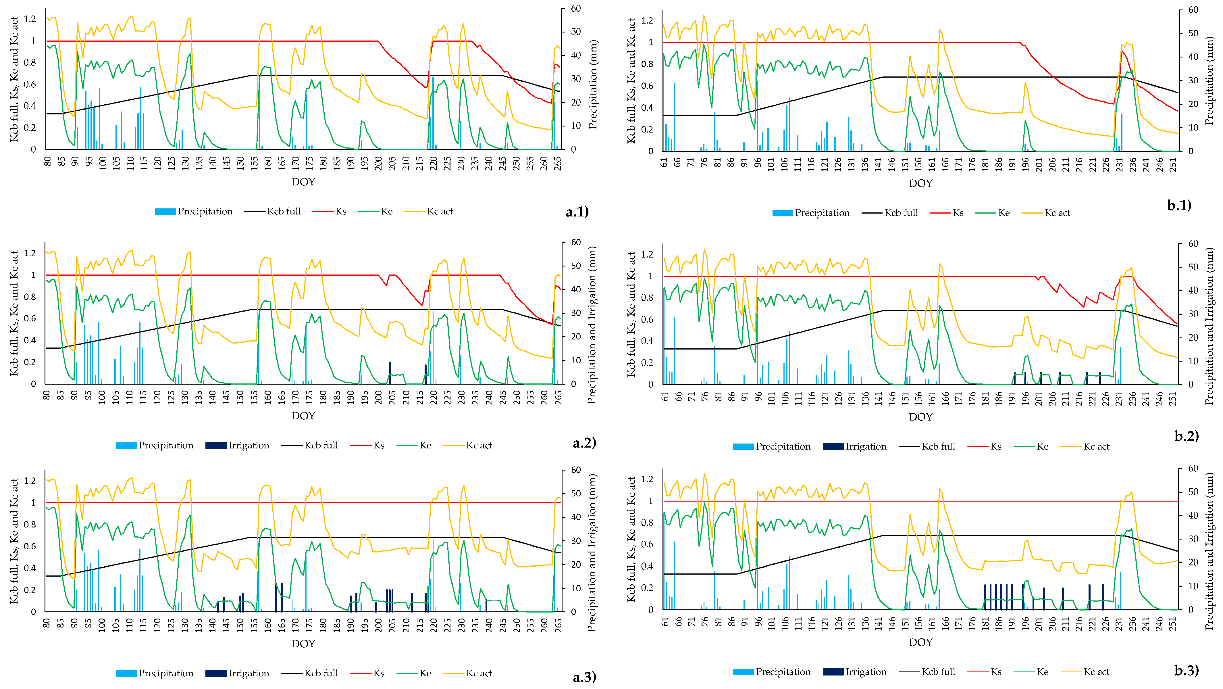
The variations of the different coefficients K_e, K_{cb full}, and K_{c act} are shown in Figure 3, along with the values of precipitation and irrigations. In Figure 3, for each treatment, the stress level (K_s) varied between 0 (maximum stress) and 1 (no stress). In the R and DI treatments, values lower than 1 were obtained in both seasons.

The total evaporable water (TEW) used was 17 mm, while the readily evaporable water (REW) used was 10 mm, and the depth of the soil evaporation layer (Z_e) was 0.1 m.

The effect of ground cover variations (Table A1) in K_{cb gcover} was negligible and limited to values 0.15–0.27 for both seasons (

Table 4. Average values of crop coefficients (-) and precipitation (mm) for different crop growth stages.

Crop Growth Stages	2019
	Dates	Kcb gcover	Kcb crop	Kcb (gcover+crop) act			Ke			Prec. (mm)
				R	DI	FI	R	DI	FI
Initial	21 May/25 May	0.26	0.00	0.26	0.26	0.26	0.93	0.93	0.93	0
Rapid growth	26 May/5 June	0.24	0.13	0.37	0.37	0.37	0.40	0.40	0.42	238
Midseason	6 June/1 September	0.27	0.21	0.45	0.47	0.48	0.22	0.23	0.27	131
End season	2 September/23 September	0.15	0.27	0.25	0.31	0.42	0.10	0.10	0.10	25
	2020
	Dates	Kcb gcover	Kcb crop	Kcb (gcover+crop) act			Ke			Prec. (mm)
				R	DI	FI	R	DI	FI
Initial	1 May/27 May	0.27	0.00	0.27	0.27	0.27	0.83	0.83	0.83	122
Rapid growth	28 May/21 June	0.25	0.09	0.33	0.33	0.33	0.52	0.52	0.52	206
Midseason	22 June/19 August	0.20	0.15	0.27	0.32	0.35	0.04	0.08	0.10	28
End season	20 August/9 September	0.17	0.22	0.21	0.30	0.39	0.19	0.20	0.21	0
Average 2019–2020		0.23	0.13	0.30	0.38	0.40	0.40	0.41	0.42	375.1

K_{cb gcover} = basal crop coefficient of ground cover, K_{cb crop} = basal crop coefficient of vineyard, K_{cb (gcover+crop) act} = actual basal crop coefficient, K_e = soil evaporation coefficient, Prec. = precipitation (mm). R = rainfed, DI = deficit irrigation, and FI = full irrigation treatments.

). Annual climate conditions modify the K_{cb crop}, mainly during midseason and end season, with higher values in 2019 than in 2020. In the case of K_{cb (gcover+crop) act} and K_e, similar values were achieved during initial and rapid growth growing seasons for both study years (2019 and 2020). To K_{cb (gcover+crop) act,} higher values were determined to FI, with respect to DI, where R treatment showed lower values, to mid and end season. The average K_e values to R treatment were lower than DI and FI treatments during midseason, with slight differences during the end season. The values of K_e during the crop growing stages are directly proportional to SWC.

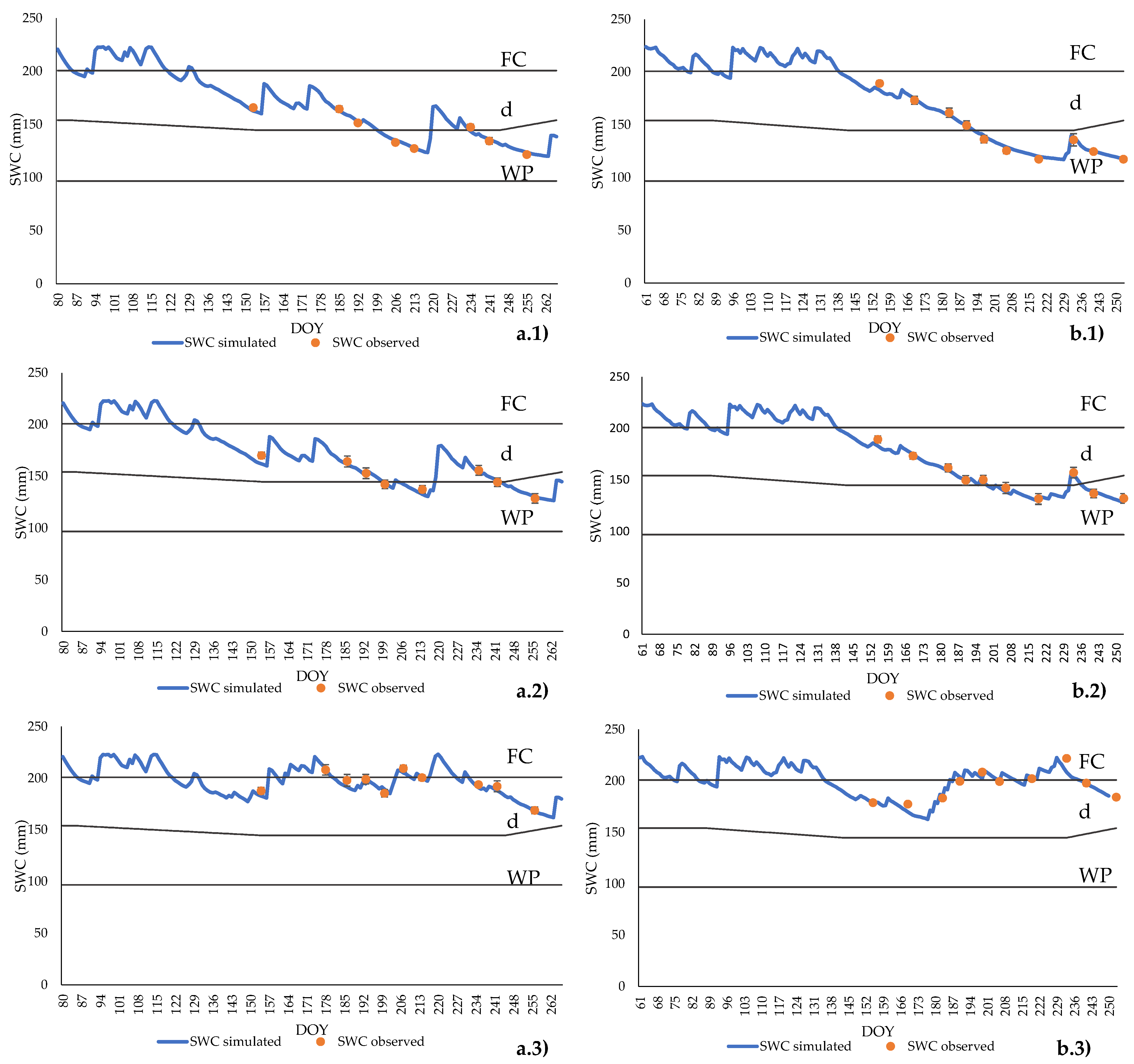
The results of the observed and simulated SWC values in R 2019, as well as the validation data, can be seen in Figure 4.

In Figure 4, the RAW value was 45 mm at the initial stage, however as the crop approached the midseason, this value increased progressively until reaching 54 mm, remaining stable until the moment of the beginning of maturation, then, it decreased again to 45 mm at the final stage.

The results of the set of goodness-of-fit indicators used to assess model fitting during calibration and to evaluate the validation results are presented in

Table 5. Goodness-of-fit indicators relative to the SIMDualKc model calibration and validations for the different treatments in the 2019 and 2020 growing seasons.

	Year	2019			2020
	Treatment	R	DI	FI	R	DI	FI
Linear regression	b	0.99	0.99	0.99	1.00	0.99	1.00
	r2	0.97	0.96	0.92	0.99	0.98	0.93
Goodness-of-fit indicators	EF	0.96	0.92	0.93	0.98	0.97	0.93
	RMSE (mm)	2.89	3.67	3.81	2.87	3.12	3.48
	NRMSE (%)	2.02	2.46	1.96	2.01	2.05	1.78
	PBIAS (%)	0.57	1.28	0.79	−0.34	0.91	0.13
	dIA	0.99	0.98	0.98	1.00	0.99	0.98
	AAE (mm)	2.26	2.92	2.66	2.21	2.69	2.99

R: rainfed; DI: deficit irrigation; FI: full irrigation; b: regression coefficient, r²: determination coefficient, EF: modeling efficiency; RMSE: root mean square error, NRMSE (%): normalized RMSE of total available water, PBIAS (%): percent bias of estimation; dIA: index of agreement; AAE: average absolute error (mm). Underlined data refer to calibration.

. In Table 5, the column of the underlined values refers to the calibration performed for the R-2019 treatment, as well as the validations for the other treatments. The b and r² values resulting from a forced regression to the origin can be observed, and the values of the indicators EF, RMSE, NRMSE (%), PBIAS (%), dIA, and AAE were obtained from the package of equations presented above (Equations (10)–(15)). The results for the regression coefficient b varied from 0.99 to 1.00, reaching close to 1.0, indicating that predicted and observed values were statistically similar for all crop seasons. The r² values ranged from 0.92 to 0.98, indicating that most of the total variance of the observed values was explained by the model. The RMSE values are quite low, ranging from 2.87 to 3.81 mm, indicating that the errors of estimation were small, representing values lower than 3.9% of the TAW. These values, combined with the low NRMSE (ranging from 1.78 to 2.46), indicate low residual errors. The AAE values were also quite small, ranging between 2.21 and 2.99 mm. The PBIAS were very low, indicating a slight underestimation bias in the calibration treatment (PBIAS = 0.57) and a moderate (PBIAS = 1.28) overestimation bias in DI treatment in 2019. Thus, the model did not show a trend for under or overestimation bias.

4. Discussion

The values obtained in this study for the HI index were higher than those observed in a study carried out with Vitis vinifera cv. Albariño in Rías Baixas (HI average of 1955.6 °C), Spain [46] (northwest Iberian Peninsula). This result indicates that in this region, the temperatures recorded were globally higher; this can be an indicator that distinguishe the regions. Regarding the CI index, it is possible to observe that the average minimum temperatures in September were higher in the Rías Baixas region (average of 14.7 °C) [46]. The Winkler (WI) and Huglin (HI) indices show that temperatures were lower in the year 2019 (Table 1). Associated with these lower temperatures, there was also a slightly lower annual precipitation value, and therefore, the values obtained with the application of the Seljaninov (SI) and Branas (BI) indices were very different in the two years, obtaining in 2019 a higher SI and a lower BI (Table 1). These indexes can explain the differences obtained in K_{c act}. As can be observed in Figure 3, the curve of K_{c act} in strategy R in 2020 (warmest year) generally presents lower values when compared to the same strategy in 2019. The result of SI and BI also explains the lower SWC values in strategy R in 2020 when compared to R in 2019 (Table 1) as well as longer stress periods (Figure 4).

Regarding the standard values, the initial and midseason differences can be compared with the calibrated values. In addition to these differences in the cultural coefficients, the best fit was obtained with equal p depletion fractions, except in midseason. During the midseason, a higher value of p depletion fraction was used, which means that the midseason culture of Vitis vinifera cv. Loureiro is less tolerant to water stress than mentioned by the authors of [6] for the generality of Vitis vinifera cultivars.

Through Figure 3, it is possible to find moments in the R vineyards (Figure 3(a1,b1)), that were subject to long periods of water stress (K_s < 1); however, in DI vineyards (Figure 3(a2,b2)), the stress periods are lower and have also shorter duration due to the irrigations adding up to compensate water shortages. In FI vineyards, in both years (Figure 3(a3,b3)) there were no moments of water stress. Moreover, in Figure 3, it is possible to find moments, (especially at the initial growth stages) when the K_e values are very similar to K_{c act}, close to 1.2. This fact is observed due to the high rainfall that occurred during these periods (Table 4) as well as the existence of low or no density and height of the soil cover vegetation. Similar trends in K_e and K_c values were observed by the authors of [26], to ‘Godello’ and ‘Mencía’ cultivars in Galicia, NW Spain.

Through the analysis of the results for the two seasons and three treatments (Table 4), K_{cb gcover} and K_{cb crop}, during the mid and end seasons, were limited to their potential values due to long periods of water stress, mainly in R and DI treatments. K_{cb (gcover+crop) act} during the initial stage (0.26), were lower than previous values reported by the authors of [20,47] (≈0.60). During the midseason, the values obtained for the K_{cb (gcover+crop) act} (0.42) were lower than those presented by the authors of [20], which collected values of 0.65 in this period. This aspect is related to the vineyard management of the Albariño, conducted in a semi-trellised system, compared to the trellis system of the Loureiro in our study. On the contrary, in the end season, slightly higher mean values of K_{cb (gcover+crop) act} are obtained for the FI treatment (0.41), being similar for the DI treatment (0.30) compared to the mean value obtained by Fandiño et al. [20] (K_{cb (gcover+crop) act} = 0.30). The higher values in FI treatment are due to a greater vegetative development of the vineyard during end season, where a K_{cb crop} was obtained (0.25), compared to the lower value, obtained by Fandiño et al. [20], with an average value of 0.14, but similar to the work of [26] with K_{cb vine end} of 0.22, to ‘Godello’ and ‘Mencía’ cultivars in Galicia, NW Spain.

In relation to basal crop coefficients, similar values of K_{cb crop} (0.18) during the midseason were obtained by Yunusa et al. [47] (0.17) to ‘Sultana’ vineyard with a 40% of ground cover in Australia. Other authors reported higher values for K_{cb mid} in wine grapes: the authors of [26] report K_{cb vine mid} = 0.25, the work of [48] reports K_{cb mid} around 0.50. However, K_{cb crop end} is much smaller than values reported by the authors of [48] in a ‘Riesling’ vineyard in the New York State, USA, who found K_{cb crop end} values of 0.55.

In Figure 4, a suitable approximation between the simulated and measured SWC values can be observed, indicating that the model can predict the SWC values throughout the vineyard season using the various irrigation strategies. The values obtained by the capacitive probe demonstrate the existence of a very low error, so we can conclude that the amount of water in the soil did not vary significantly between repetitions. The K_{cb full ini} (0.33) calibrated value was slightly higher to the initial period than values obtained by the authors of [20] (0.30) and relative higher to FAO-56 [6] standard values (0.20). This value is higher depending on the rainfall and active ground cover conditions. To the midseason, K_{cb full mid} value (0.684) was lower than values obtained by the authors of [20] (1.15) and [26] (0.75), mainly due to active ground cover conditions and crop development. Similarly, to end season, lower values were obtained to K_{cb full end} (0.54) when compared with [20] (0.90) and [26] (0.60). Final report values to K_{cb full} were near to ‘Godello’ and ‘Mencia’ cultivars values, with similar trellis management, so that the vineyard management (trellis and active ground cover) is presented as a key factor to select the correct crop coefficients when not available to use, instead of standard values of FAO-56 [6].

The indicators obtained from the forced regression to the origin show a suitable agreement between the observed and the simulated data. The other indicators (EF, RMSE, NRMSE, PBIAS, d_IA, and AAE) demonstrate that, after a previous calibration, the model can efficiently predict the SWC throughout the crop cycle using the various irrigation strategies. The b and r² values in the present work are better than those reported by the authors of [26], who obtained b values between 0.92 and 1.04, and r² values between 0.87 and 0.97 for grapevine with active ground cover. The efficiency of the model (EF) in the present study ranged between 0.92 and 0.97, whereas the authors of [26] obtained slightly lower values between 0.77 and 0.96. The results obtained in this work are similar to those obtained with other methodologies, for example, with the results obtained by the authors of [11], who also studied vine culture. However, the accuracy of the double model approach was verified using lysimeters and with the results obtained for the cultivation of Arbequina olive [9].

Considering the totality of the indicators calculated to assess the robustness of the model, it is possible to verify that, whatever the irrigation strategy (R, DI, or FI) or year of cultivation (2019 or 2020), the values obtained by these indicators indicate a suitable fit of the model.

5. Conclusions

Considering the specific parameters of the study field (soil, climate, crop, and irrigation), the calibration and validation of the SIMDualKc model were successfully performed for Vitis vinifera cv. Loureiro. In the 2 years of the field studies, 2019 and 2020, a goodness of fit was obtained between the SWC values observed with a capacitive probe and those simulated with the SIMDualKc model.

After making the necessary adjustments to the standard values [6], we obtained a suitable approximation between the real and simulated values. We conclude that the application of the dual approach with the SIMDualKc model is possible because, as other authors have noted, the model can correctly predict the SWC.

These values enable the determination of the SWC in future growth seasons, facilitating irrigation management by allowing farmers to adapt their management practices to achieve the levels of water stress that they want for their vineyard.

The use of calibrated parameters for cv. Loureiro allows farmers to efficiently use water. However, it is still necessary to carry out studies in the future to determine the vine response to the different levels of water stress generated in each irrigation treatment.

To facilitate the application of this calibration, it is recommended to round the values of K_{cb full ini}, K_{cb full mid}, and K_{cb full end} to 0.35, 0.70, and 0.55, respectively.

References

- Oliveira, A.F.; Mameli, M.G.; Cascio, M.L.; Sirca, C.; Satta, D. An Index for User-Friendly Proximal Detection of Water Requirements to Optimized Irrigation Management in Vineyards. Agronomy 2021, 11, 323. [Google Scholar] [CrossRef]
- Kim, S.; Meki, M.N.; Kim, S.; Kiniry, J.R. Crop modeling application to improve irrigation efficiency in year-round vegetable production in the texaswinter garden region. Agronomy 2020, 10, 1525. [Google Scholar] [CrossRef]
- Nesheim, I.; Barkved, L. The suitability of the ecosystem services framework for guiding benefit assessments in human-modified landscapes exemplified by regulated watersheds-Implications for a sustainable approach. Sustainability 2019, 11, 1821. [Google Scholar] [CrossRef] [Green Version]
- Islam, S.M.F.; Karim, Z. World’s Demand for Food and Water: The Consequences of Climate Change. IntechOpen 2019, 13. [Google Scholar] [CrossRef] [Green Version]
- Pereira, L.S.; Oweis, T.; Zairi, A. Irrigation management under water scarcity. Agric. Water Manag. 2002, 57, 175–206. [Google Scholar] [CrossRef]
- Allen, R.G.; Pereira, L.S.; Smith, M.; Raes, D. Crop Evapotranspiration. Guide- lines for Computing Crop Water Requirements Paper 56. FAO Irrig. Drain. 1998, 300, D05109. [Google Scholar]
- Pereira, L.S.; Paredes, P.; Melton, F.; Johnson, L.; Wang, T.; López-Urrea, R.; Cancela, J.J.; Allen, R.G. Prediction of crop coefficients from fraction of ground cover and height. Background and validation using ground and remote sensing data. Agric. Water Manag. 2020, 241, 106197. [Google Scholar] [CrossRef]
- Paço, T.A.; Pôças, I.; Cunha, M.; Silvestre, J.C.; Santos, F.L.; Paredes, P.; Pereira, L.S. Evapotranspiration and crop coefficients for a super intensive olive orchard. An application of SIMDualKc and METRIC models using ground and satellite observations. J. Hydrol. 2014, 519, 2067–2080. [Google Scholar] [CrossRef] [Green Version]
- Paço, T.A.; Paredes, P.; Pereira, L.S.; Silvestre, J.; Santos, F.L. Crop coefficients and transpiration of a super intensive Arbequina olive orchard using the dual Kc approach and the Kcb computation with the fraction of ground cover and height. Water 2019, 11, 383. [Google Scholar] [CrossRef] [Green Version]
- López-Urrea, R.; Sánchez, J.M.; de la Cruz, F.; González-Piqueras, J.; Chávez, J.L. Evapotranspiration and crop coefficients from lysimeter measurements for sprinkler-irrigated canola. Agric. Water Manag. 2020, 239, 106260. [Google Scholar] [CrossRef]
- López-Urrea, R.; Montoro, A.; Mañas, F.; López-Fuster, P.; Fereres, E. Evapotranspiration and crop coefficients from lysimeter measurements of mature “Tempranillo” wine grapes. Agric. Water Manag. 2012, 112, 13–20. [Google Scholar] [CrossRef]
- Rallo, G.; Provenzano, G.; Castellini, M.; Sirera, À.P. Application of EMI and FDR sensors to assess the fraction of transpirable soil water over an olive grove. Water 2018, 10, 168. [Google Scholar] [CrossRef] [Green Version]
- Provenzano, G.; Rallo, G.; Ghazouani, H. Assessing Field and Laboratory Calibration Protocols for the Diviner 2000 Probe in a Range of Soils with Different Textures. J. Irrig. Drain. Eng. 2016, 142, 04015040. [Google Scholar] [CrossRef]
- Zhuang, Q.; Wu, S.; Feng, X.; Niu, Y. Analysis and prediction of vegetation dynamics under the background of climate change in Xinjiang, China. PeerJ 2020, 8, e8282. [Google Scholar] [CrossRef]
- Garcia, L.; Celette, F.; Gary, C.; Ripoche, A.; Valdés-Gómez, H.; Metay, A. Management of service crops for the provision of ecosystem services in vineyards: A review. Agric. Ecosyst. Environ. 2018, 251, 158–170. [Google Scholar] [CrossRef] [Green Version]
- Lopes, C.M.; Santos, T.P.; Monteiro, A.; Rodrigues, M.L.; Costa, J.M.; Chaves, M.M. Combining cover cropping with deficit irrigation in a Mediterranean low vigor vineyard. Sci. Hortic. 2011, 129, 603–612. [Google Scholar] [CrossRef] [Green Version]
- Gattullo, C.E.; Mezzapesa, G.N.; Stellacci, A.M.; Ferrara, G.; Occhiogrosso, G.; Petrelli, G.; Castellini, M.; Spagnuolo, M. Cover crop for a sustainable viticulture: Effects on soil properties and table grape production. Agronomy 2020, 10, 1334. [Google Scholar] [CrossRef]
- Pou, A.; Gulías, J.; Moreno, M.; Tomás, M.; Medrano, H.; Cifre, J. Cover cropping in Vitis vinifera L. cv. Manto Negro vineyards under Mediterranean conditions: Effects on plant vigour, yield and grape quality. J. Int. Des Sci. La Vigne Du Vin 2011, 45, 223–234. [Google Scholar] [CrossRef] [Green Version]
- Sivcev, B.; Sivcev, I.; Rankovic-Vasic, Z. Plant protection products in organic grapevine growing. J. Agric. Sci. Belgrade 2010, 55, 103–122. [Google Scholar] [CrossRef]
- Fandiño, M.; Cancela, J.J.; Rey, B.J.; Martínez, E.M.; Rosa, R.G.; Pereira, L.S. Using the dual-K c approach to model evapotranspiration of Albariño vineyards (Vitis vinifera L. cv. Albariño) with consideration of active ground cover. Agric. Water Manag. 2012, 112, 75–87. [Google Scholar] [CrossRef]
- French, A.N.; Hunsaker, D.J.; Sanchez, C.A.; Saber, M.; Gonzalez, J.R.; Anderson, R. Satellite-based NDVI crop coefficients and evapotranspiration with eddy covariance validation for multiple durum wheat fields in the US Southwest. Agric. Water Manag. 2020, 239, 106266. [Google Scholar] [CrossRef]
- Raes, D. Book I: Understanding AquaCrop; FAO: Rome, Italy, 2017; ISBN 9789251093900. [Google Scholar]
- Rosa, R.D.; Paredes, P.; Rodrigues, G.C.; Fernando, R.M.; Alves, I.; Pereira, L.S.; Allen, R.G. Implementing the dual crop coefficient approach in interactive software: 2. Model testing. Agric. Water Manag. 2012, 103, 62–77. [Google Scholar] [CrossRef]
- Rolim, J.; Godinho, P.; Sequeira, B.; Paredes, P.; Pereira, L.S. Assessing the SIMDualKc model for irrigation scheduling simulation in Mediterranean environments. Water Sav. Mediterr. Agric. Futur. Res. Needs 2007, 1, 49–61. [Google Scholar]
- Fandiño, M.; Olmedo, J.L.; Martínez, E.M.; Valladares, J.; Paredes, P.; Rey, B.J.; Mota, M.; Cancela, J.J.; Pereira, L.S. Assessing and modelling water use and the partition of evapotranspiration of irrigated hop (Humulus Lupulus), and relations of transpiration with hops yield and alpha-acids. Ind. Crops Prod. 2015, 77, 204–217. [Google Scholar] [CrossRef]
- Cancela, J.J.; Fandiño, M.; Rey, B.J.; Martínez, E.M. Automatic irrigation system based on dual crop coefficient, soil and plant water status for Vitis vinifera (cv Godello and cv Mencía). Agric. Water Manag. 2015, 151, 52–63. [Google Scholar] [CrossRef]
- Allen, R.G.; Pruitt, W.O.; Wright, J.L.; Howell, T.A.; Ventura, F.; Snyder, R.; Itenfisu, D.; Steduto, P.; Berengena, J.; Yrisarry, J.B.; et al. A recommendation on standardized surface resistance for hourly calculation of reference ETo by the FAO56 Penman-Monteith method. Agric. Water Manag. 2006, 81, 1–22. [Google Scholar] [CrossRef]
- Allen, R.G.; Clemmens, A.J.; Burt, C.M.; Solomon, K.; O’Halloran, T. Prediction Accuracy for Projectwide Evapotranspiration Using Crop Coefficients and Reference Evapotranspiration. J. Irrig. Drain. Eng. 2005, 131, 24–36. [Google Scholar] [CrossRef] [Green Version]
- Allen, R.G.; Pereira, L.S. Estimating crop coefficients from fraction of ground cover and height. Irrig. Sci. 2009, 28, 17–34. [Google Scholar] [CrossRef] [Green Version]
- Rallo, G.; Paço, T.A.; Paredes, P.; Puig-Sirera, À.; Massai, R.; Provenzano, G.; Pereira, L.S. Updated single and dual crop coefficients for tree and vine fruit crops. Agric. Water Manag. 2021, 250, 106645. [Google Scholar] [CrossRef]
- Pereira, L.S.; Paredes, P.; Hunsaker, D.J.; López-Urrea, R.; Jovanovic, N. Updates and advances to the FAO56 crop water requirements method. Agric. Water Manag. 2021, 248, 106697. [Google Scholar] [CrossRef]
- Fraga, H.; Malheiro, A.C.; Moutinho-Pereira, J.; Santos, J.A. Climate factors driving wine production in the Portuguese Minho region. Agric. For. Meteorol. 2014, 185, 26–36. [Google Scholar] [CrossRef]
- Kottek, M.; Grieser, J.; Beck, C.; Rudolf, B.; Rubel, F. World map of the Köppen-Geiger climate classification updated. Meteorol. Zeitschrift 2006, 15, 259–263. [Google Scholar] [CrossRef]
- Cardoso, A.S.; Alonso, J.; Rodrigues, A.S.; Araújo-Paredes, C.; Mendes, S.; Valín, M.I. Agro-ecological terroir units in the North West Iberian Peninsula wine regions. Appl. Geogr. 2019, 107, 51–62. [Google Scholar] [CrossRef]
- Winkler, A.J.; Cook, J.A.; Kliewer, W.M.; Lider, L.A. General Viticulture, 4th ed.; University of California Press: Berkley, CA, USA, 1974; ISBN 9780520025912. [Google Scholar]
- Huglin, P. Nouveau mode d’évaluation des possibilités héliothermiques d’un milieu viticole. Comptes Rendus L’académie D’agriculture Fr. 1978, 64, 1117–1126. [Google Scholar]
- Tonietto, J. Les Macroclimats Viticoles Mondiaux et L’influence du Mésoclimat sur la Typicité de la Syrah et du Muscat de Hambourg dans le Sud de la France: Méthodologie de Caráctérisation; Ecole Nationale Superieure Agronomique De Montpellier: E.N.S.A: Montpellier, France, 1999. [Google Scholar]
- Seljaninov, G.T. Agroclimatic Map of the World; Hydrometeoizdat Publishing House: Leningrad, Russia, 1966. [Google Scholar]
- Branas, J.; Bernon, G.; Levadoux, L. Eléments de Viticulture Générale; Imp. Dehan: Bordeaux, France, 1946. [Google Scholar]
- WRB World Reference Base for Soil Resources. World Soil Resources Reports 106; FAO: Rome, Italy, 2014; ISBN 9789251083697. [Google Scholar]
- Evett, S.R.; Stone, K.C.; Schwartz, R.C.; O’Shaughnessy, S.A.; Colaizzi, P.D.; Anderson, S.K.; Anderson, D.J. Resolving discrepancies between laboratory-determined field capacity values and field water content observations: Implications for irrigation management. Irrig. Sci. 2019, 37, 751–759. [Google Scholar] [CrossRef] [Green Version]
- Liu, Y.; Pereira, L.S.; Fernando, R.M. Fluxes through the bottom boundary of the root zone in silty soils: Parametric approaches to estimate groundwater contribution and percolation. Agric. Water Manag. 2006, 84, 27–40. [Google Scholar] [CrossRef]
- Rosa, R.D.; Paredes, P.; Rodrigues, G.C.; Alves, I.; Fernando, R.M.; Pereira, L.S.; Allen, R.G. Implementing the dual crop coefficient approach in interactive software. 1. Background and computational strategy. Agric. Water Manag. 2012, 103, 8–24. [Google Scholar] [CrossRef]
- Baggiolini, M.; Lorenz, H.; Bleiholder, H.; T., V.D.B.; Stauss, R.; Weber, E.; Witzenberger, A.; Hack, H.; Bleiholder, H.; Buhr, L.; et al. Stades phénologiques repères de la vigne. Arboric. Hortic. 1993, 44, 7–9. [Google Scholar]
- Paredes, P.; Rodrigues, G.J.; Petry, M.T.; Severo, P.O.; Carlesso, R.; Pereira, L.S. Evapotranspiration partition and crop coefficients of Tifton 85 bermudagrass as affected by the frequency of cuttings. Application of the FAO56 dual Kc model. Water 2018, 10, 558. [Google Scholar] [CrossRef] [Green Version]
- Cancela, J.J.; Trigo-Córdoba, E.; Martínez, E.M.; Rey, B.J.; Bouzas-Cid, Y.; Fandiño, M.; Mirás-Avalos, J.M. Effects of climate variability on irrigation scheduling in white varieties of Vitis vinifera (L.) of NW Spain. Agric. Water Manag. J. 2016, 170, 99–109. [Google Scholar] [CrossRef]
- Yunusa, I.A.M.; Walker, R.R.; Guy, J.R. Partitioning of seasonal evapotranspiration from a commercial furrow-irrigated Sultana vineyard. Irrig. Sci. 1997, 18, 45–54. [Google Scholar] [CrossRef]
- Intrigliolo, D.S.; Lakso, A.N.; Piccioni, R.M. Grapevine cv. “Riesling” water use in the northeastern United States. Irrig. Sci. 2009, 27, 253–262. [Google Scholar] [CrossRef]
Figure 1.
Daily weather data recorded in the field relative to (a) maximum (Tmax, °C) and minimum (Tmin, °C) temperatures; (b) minimum relative humidity (RHmin, %), wind speed at 2 m height (U2, m s−1) and (c) precipitation and reference evapotranspiration (ETo, mm d−1) for the period 2019–2020.
Figure 2.
Position of the access probe tubes located in full irrigation ( ![Agronomy 11 02062 i001]() ), deficit irrigation (
), deficit irrigation ( ![Agronomy 11 02062 i002]() ), and rain-feed (
), and rain-feed ( ![Agronomy 11 02062 i003]() ) treatments (a). A schematic view of vines, emitters, and access probe tubes (b).
) treatments (a). A schematic view of vines, emitters, and access probe tubes (b).
), deficit irrigation (
), and rain-feed (
), deficit irrigation ( ), and rain-feed ( ) treatments (a). A schematic view of vines, emitters, and access probe tubes (b).
Figure 3.
Precipitation ( ![Agronomy 11 02062 i004]() ), irrigation (
), irrigation ( ![Agronomy 11 02062 i005]() ) Kcb full (
) Kcb full ( ![Agronomy 11 02062 i006]() ), Ks (
), Ks ( ![Agronomy 11 02062 i007]() ), Ke (
), Ke ( ![Agronomy 11 02062 i008]() ), and Kc act (
), and Kc act ( ![Agronomy 11 02062 i009]() ) and relative to the: (a) year 2019, (b) year 2020; (1) rainfed (R), (2), deficit irrigation (DI), (3) full irrigation (FI).
) and relative to the: (a) year 2019, (b) year 2020; (1) rainfed (R), (2), deficit irrigation (DI), (3) full irrigation (FI).
), irrigation (
) Kcb full (
), Ks (
), Ke (
), and Kc act (
), irrigation ( ) Kcb full ( ), Ks ( ), Ke ( ), and Kc act ( ) and relative to the: (a) year 2019, (b) year 2020; (1) rainfed (R), (2), deficit irrigation (DI), (3) full irrigation (FI).
Figure 4.
Simulated ( ![Agronomy 11 02062 i010]() ) vs. observed (
) vs. observed ( ![Agronomy 11 02062 i011]() ) average available soil water content (SWC) relative to the: (a) year 2019, (b) year 2020; (1) rainfed (R), (2) deficit irrigation (DI), (3) full irrigation (FI). DOY represents the day of the year. Error bars represent the standard deviation of the mean observed values. Curves FC, WP, and d represent the soil water content at field capacity, wilting point, and d the soil water content when depletion equals the p fraction, respectively.
) average available soil water content (SWC) relative to the: (a) year 2019, (b) year 2020; (1) rainfed (R), (2) deficit irrigation (DI), (3) full irrigation (FI). DOY represents the day of the year. Error bars represent the standard deviation of the mean observed values. Curves FC, WP, and d represent the soil water content at field capacity, wilting point, and d the soil water content when depletion equals the p fraction, respectively.
) vs. observed (
) vs. observed ( ) average available soil water content (SWC) relative to the: (a) year 2019, (b) year 2020; (1) rainfed (R), (2) deficit irrigation (DI), (3) full irrigation (FI). DOY represents the day of the year. Error bars represent the standard deviation of the mean observed values. Curves FC, WP, and d represent the soil water content at field capacity, wilting point, and d the soil water content when depletion equals the p fraction, respectively.