Assessing and Modeling Ecosystem Carbon Exchange and Water Vapor Flux of a Pasture Ecosystem in the Temperate Climate-Transition Zone

Abstract

The rising frequency of extreme weather events and global warming are greatly challenging pastoral ecosystem productivity, particularly in the temperate climate-transition regions. While this could cause greater gross primary production (GPP) mainly contributed by the warm-season vegetation, the consequences for the dynamics of net ecosystem exchange (NEE) and hydrological responses (e.g., evapotranspiration, ET) on an ecosystem level are poorly known. Here, we investigated the evolution of plant phenology, nutritive value, energy balance, and carbon/water budgets of a cool-season dominated pastoral ecosystem in the temperate zone; integrating both eddy covariance (EC) flux measurement and simulation modeling-based uncertainty analysis. Throughout the two-year duration (2017–2018) of this study, the entire pasture ecosystem remained a strong carbon sink (NEE = −1.23 and −1.95 kg C m⁻², respectively) with 74% and 62% of available energy loss explained by EC fluxes, respectively. The cumulative ET was 735.8 and 796.8 mm, respectively; and the overall ecosystem water use efficiency (EWUE) were calculated as 6.5 g C kg⁻¹ water across both growing seasons. The above-ground biomass yield agreed with the cumulative GPP and was inversely correlated with grass nutritive value. The uncertainty analysis indicated that accurate EC flux gap-filling models could be constructed using support vector machine trained time-series models (NEE, R² = 0.77, RMSE = 11.8; ET, R² = 0.90, RMSE = 73.8). The performance benchmarking tests indicated that REddyProc-based gap-filling performance was very limiting and highly variable (NEE, R² = 0.21–0.64; ET, R² = 0.79–0.87), particularly for estimating NEE. Overall, the warm-season vegetation encroachment greatly filled the production gap of cool-season grasses, leading to greater cumulative NEE and EWUE on a system level, compared with those from many other reported field-crop or grassland studies using EC approaches. The complex and dynamic nature of grassland ecosystems greatly challenged the conventional REddyProc-based EC flux gap-filling performance. However, accurate machine learning models could be constructed for error/uncertainty control purposes and, thus, should be encouraged in future studies.

1. Introduction

Pasture ecosystems serve important functions in providing high-quality feed to herbivores, producing biofuel feedstocks, and offering great ecological services such as carbon sequestration and biodiversity. However, the resilience and sustainability of these ecosystems have been challenged by climate change, weed encroachment, and anthropogenic intervention; leading to great uncertainties over the carbon/water budget and energy balance dynamics on a system level [1,2,3]. Thus, capturing and modeling the carbon/water vapor footprints of these pasture ecosystems using advanced instrumentation methods and computational approaches could greatly enhance our understanding of ecosystem functioning and behavior under the changing climate conditions.

Located in the middle of a climate transition zone, the middle Tennessee region has excellent weather conditions for plant production. In particular, several cool-season grass species such as tall-fescue (Lolium arundinaceum (Schreb.) Darbyish.), orchardgrass (Dactylis glomerata L.), and kentucky bluegrass (Poa pratensis L.) are well adapted to the soil and climate conditions in this interfacing environment between the northeast and southeast vegetation zones [4,5]. These plant species, together with many introduced and/or native warm-season grasses, make this temperate transition zone one of the most productive and diverse plant production regions in the world. Most importantly, these cool-season dominated pasture ecosystems are very sensitive to rising temperatures and drought conditions, evidenced by increasing encroachment of warm-season species in the summer, and rising frequency and intensity of insect and weed outbreaks. These characteristics provide us with excellent candidate ecosystems to investigate the dynamics and behaviors of carbon/water vapor footprints along with their interactions with various environmental/ecological factors and legacy effects.

Numerous studies were conducted previously to explore how carbon fluxes and/or ecosystem productivity respond to different managerial factors or species composition within pasture ecosystems [6,7,8,9,10]. For example, Skinner [9] found that season alterations (winter vs. summer) can significantly impact ecosystem productivity and carbon balance of cool-season pasture ecosystems. Hunt et al. [6] reported that the net ecosystem carbon budget of a ryegrass (Lolium perenne L.) and clover (Trifolium repens L.) dominated dairy pasture could be greatly altered by irrigation input or grazing activities. Likewise, Zhou et al. [10] found that carbon dynamics of an old world bluestem (Bothriochloa caucasica C. E. Hubb.) pasture depended greatly on interactions between climatic (e.g., precipitation pattern) and managerial interactions (e.g., fertilization and hay harvest). These studies have provided updated evidence regarding how a pasture ecosystem responds to various biotic and abiotic factors. However, very few studies simultaneously investigated both carbon and water budgets; and a very crucial piece of information relating to uncertainty analysis of flux data using advanced simulation modeling approaches was extremely limited [6] and even non-existent in the temperate climate transition pasture ecosystems.

Kallenbach [11] and Hunt et al. [6] noted that the nutrient cycling processes and carbon balance dynamics of pasture ecosystems are very complex and could be governed by many exogenous factors and interactions. In light of this, the main goals for this study were to: (i) quantify and characterize how inter-annual climatic changes and management practices could affect water, carbon, and energy dynamics of a cool-season dominated pasture ecosystem in the climate transition area; (ii) conduct uncertainty analysis of flux data gap-filling capacity using different driver variables and machine learning algorithms, and benchmark the results against well-established methods. We postulated that carbon and water fluxes of such systems should be very complex, which could greatly challenge the modeling performance. Meanwhile, we also hypothesized that accurate flux data gap-filing models could be constructed using high-quality eddy covariance (EC) data in conjunction with machine learning algorithms.

2. Material and Methods

2.1. Study Site Description

The study was conducted at Lascassas, TN, USA. The primary soil type was Hillwood gravelly silt loam (12% to 20% slopes, Alfisol, thermic Oxyaquic Fraglossudalf). The long-term (>30 years) average annual precipitation and mean annual temperature were 1397 mm and 15 °C, respectively. The entire pasture was measured as 12.8 ha with the geometric center located at the latitude of 35°53′19.66″ N and the longitude of 86°16′23.77″ W. The grassland pasture was originally established in 2008 and was dedicated for hay production or periodical cattle grazing. It was primarily managed as a cool-season grass dominated natural pastoral ecosystem without application of chemical fertilizers, pesticides, or herbicides. No grazing activities were allowed since the establishment of the EC towers in late 2016. Biomass harvest was performed when the majority of the cool-season grasses reach boot stage. In particular, hay was harvested, cured, and baled from the entire pasture twice in (17 July and 6 September) 2017 and (15 July and 17 September) 2018. Botanical composition was evaluated before EC data collection in late 2016, indicating ~40% of tall fescue, ~10% of kentucky bluegrass, ~20% of orchardgrass, and ~30% of other forbs and legumes. Warm-season grass encroachment (35–40% of botanical composition) was typically observed during the hot summer months to early fall (July to August) mainly consisting of purpletop (Tridens flavus (L.) Hitchc.), johnsongrass (Sorghum halepense (L.) Pers.), and dallisgrass (Paspalum dilatatum Poir.); and the warm-season grass population dwindled rapidly in late fall (September to October).

The entire EC-tower system was established in late August 2016 and was continuously recording data until late August of 2018. This time window included two complete growing cycles of typical cool-season grasses which starts from the beginning of the stockpiling season (or fall-planting season) in the early autumn to the end of summer-dormancy season of the following year. In Middle Tennessee, fall-planting (from late August to Mid-September) of cool-season grasses is generally preferred for controlling weed outbreak and Sclerotinia homoeocarpa F.T. Bennett infection [12] compared to spring planting. The detailed patterns of daily average ambient air temperature (Tair), soil volumetric water content (SVWC), and precipitation during each growing season are shown in Figure 1.

In particular, the cumulative growing-season precipitation was 1212 and 1353 mm; and the average Tair was 15.8 and 14.3 °C for the first and the second growing seasons, respectively. The average SVWC was 26.6 and 31.4% with the values mostly between 8.6 to 36.2% and 18.4 to 39.7% during the two consecutive growing seasons, respectively.

2.2. Eddy Covariance Tower Establishment and Other Accessory Instruments

The instrument tower consisted of a complete EC system and other accessory meteorological sensors, including a Gill-WM WindMaster 3-D Sonic Anemometer (Gill Instruments Ltd., Lymington, Hampshire, UK, at 3 m height) and an LI-7500RS open-path infrared gas analyzer (IRGA, Li-Cor Inc., Lincoln, NE, USA at a 3 m height) integrated with the SMARTFlux System. The software estimates quality of each flux data point using a flux quality flag obtained from the integral results of the steady-state and the development turbulence tests. The flagging policy is in compliance with the documented standards specified by the ICOS (Integrated Carbon Observation System), AmeriFlux, and FLUXNET; which uses numerical values ‘0’, ‘1’, and ‘2’ to indicate high-quality, suitable for budget analysis, and poor-quality data; respectively.

Supplementary instruments were included in the LI-7900-102 Biomet System Package (Li-Cor Inc., Lincoln, NE, USA). The whole package included an NR Lite2 net Radiometer (Kipp and Zonen Corp., Delft, The Netherlands at 2.5 m height), a Vaisala HMP155 Humidity and Temperature sensor (Vaisala Corp., Helsinki, Finland at 2.8 m height) housed in an RM Young 41005-5 Radiation Shield (R.M. Young Company, Traverse City, MI, USA), three Hukseflux HFP01SC Self-Calibrating Soil Heat Flux sensors (Hukseflux Thermal Sensors, Delft, The Netherlands at 8 cm depth), three Stevens Hydra Probe II (Stevens Water Monitoring Systems Inc., Portland, OR, USA at 6 cm depth), an LI-200R Pyranometer (Li-Cor Inc., NE, USA at 2.5 m height), an LI-190R Quantum Sensor (Li-Cor Inc., NE, USA at 2.5 m height), a TR-525USW Rain/Precipitation gauge (Texas Instruments Inc., Dallas, TX, USA at 1.5 m height), and a Sutron Xlite 9210 Data logger (Sutron Corp., Sterling, VA, USA).

2.3. Flux Data Processing and Gap Filling

The daily summary logged files containing 30 min flux values were collected and stored as tab-delimited text files. The REddyProc Software Package from the Max Planck Institute for Biogeochemistry was used for flux data gap-filling and partitioning of net ecosystem exchange (NEE) into ecosystem respiration (ER) and gross primary production (GPP). In particular, the night-time based algorithms [13] were used for NEE partitioning; and the Ustar-based methods in conjunction with the Moving Point Test threshold estimation algorithms [14] were used for flux data filtering. The detailed information regarding the data filtering, gap-filling, and partitioning [13,15] could be found at the REddyProc website: https://www.bgc-jena.mpg.de/bgi/index.php/Services/REddyProcWebRPackage (accessed date: 24 January 2021). According to the sign convention for presenting NEE data, negative flux values indicate overall CO₂ sequestration (fluxes from the atmosphere to the ecosystem) and positive values indicate overall CO₂ release (fluxes from the ecosystem to the atmosphere). Throughout the entire duration of this study, 16.5% of NEE data and 15.9% of latent heat flux (LE) data were classified as “gap” either caused by missing values or identified by the Ustar-filtering algorithms. Evapotranspiration (ET) was calculated using LE based on equations described by Rajan et al. [16]. Obvious outliers (NEE beyond ±50 μmol m⁻² s⁻¹) [17,18] were removed manually from the dataset. All daily cumulative values, including NEE, ER, GPP, and ET; were calculated by integrating the value-by-seconds plotting using the “trapz” function (trapezoidal numerical integration) in MATLAB.

The energy balance and closure of the entire ecosystem were evaluated by regressing the 30 min values of total turbulent fluxes (H + LE) with the available energy accumulation [net radiation (Rn)-soil heat flux (G)] within each growing season. Specifically, non-gap-filled high-quality data, indicated by ‘0′ quality flag values for corresponding LE and H, and those ranging from −200 to 500 and from −200 to 800 W m⁻² of H and LE, respectively; were retained for this task [19,20]. After applying all filtering criteria mentioned above, 28% of data were removed from the energy balance/closure analysis. Finally, both coefficient of determination (R²) and root mean square error (RMSE) were used for model fitting assessment and the results were presented by growing season.

2.4. Plant Biomass Sampling and Nutritive Value Estimation

Plant biomass samples were taken from three 0.3 m² quadrats at a 5 cm cutting height from randomly selected locations from April to August within each growing season. Sampling dates were 13 May, 26 June, 20 July, 27 August, for the first growing season; and 12 May, 19 June, 17 July, 25 August, for the second growing season. This sampling schedule was designed to avoid winter dormancy seasons and to effectively capture the end-of-spring growth of cool-season grasses, summer growth of the majority of warm-season grasses, and the biomass production of cool-season grasses during stockpiling seasons within each year. All biomass samples were immediately stored in paper bags and then shipped back to the laboratory and dried in a commercial oven at 60 °C to a constant weight. Cumulative biomass production was then correlated with GPP using simple linear regression. Following dry matter measurement, all samples were ground to fine powders that could pass 1 mm screen using a Wiley mill (Comeau Technique Ltd., Vandreuil-Dorion, Quebec, Canada). All powder samples were then scanned on a Foss DS2500 (Eden Prairie, MN) near-Infrared Spectrometer using the 2017 Grass Hay calibration model developed by the NIRS Feed and Forage Consortium (Hillsboro, WI) for nutritive value analysis. Reported nutritive indices included relative feed value (RFV), crude protein (CP), acid detergent fiber (ADF), neutral detergent (NDF), ash, fat, and lignin concentration. The Global H statistical test compared the samples against the model and other samples within the database for accurate results, where all samples fit the equation with H < 3.0 and are reported accordingly [21].

2.5. Modeling-Based Uncertainty Analysis and Benchmarking

To assess the efficacy and accuracy of the REddyProc-based gap filling algorithms on NEE and LE, we implemented a series of statistical/machine learning algorithms and benchmarked our results against REddyProc-produced results. In particular, NEE and LE were of primary interests, because both variables could be directly measured by EC systems and later used for GPP/ER partitioning and ET calculation, respectively. To complete this task, we first extracted the high-quality flux data according to the u-star filtering algorithm specified by REddyProc [22] and signal intensity associated with each flux data point, which retained the 30-min flux data that have a signal intensity of at least 60% and a u-star quality flag value of “zero,” indicating high-quality data point. Following that, the entire dataset was randomly and evenly partitioned into 10 subsets of similar size (10-fold cross validation, 10-fold CV). Each time, one subset of data were removed from the whole dataset to create artificial gaps and then gap-filled by REddyProc. This process was repeated 10 times until all ReddyProc predicted data were obtained and recombined to form a complete predicted dataset, which was then regressed with the original high-quality dataset for performance evaluation. In particular, we tested three different gap-filling conditions used by REddyProc [22]; including: only the target variables (NEE or LE) are missing but Rg, Tair, and VPD are available (Rg + Tair + VPD); both Tair and VPD are missing but Rg is available (Rg); and all three variables are missing (None) by artificially removing corresponding variable from the input dataset. Meanwhile, we also implemented our own least-square-based linear models (LSLM), artificial neural network models (ANN), and SVM models for gap-filling based on the same 10-fold CV regime. Additionally, 12 easy-to-measure EC-independent (without requiring IRGA or Sonic Anemometer) driver variables (features) were selected for this task, including hour readings, Rg, Tair, Tsoil, RH, VPD, Photosynthetic Photon Flux Density, Soil Heat Flux, Rn, wind speed, precipitation, and SVWC. The rationale for this was that we wanted to evaluate the possibility for accurately predicting high-resolution (30 min) flux data just based on easy-to-measure environmental variables without relying on high-cost IRGA or sonic anemometer. For the linear model, we used the least-square leaner, sparse-reconstruction-by-separable-approximation optimizer, and lasso-based regularization. For ANN, we constructed feedforward neural net with three hidden layers with ten, eight, and five neurons within each layer, respectively. For SVM, we used Gaussian kernel with grid-search optimizer identified hyper-parameters on standardized data. Additionally, instead of using the entire nine-subset training data, we also tested the performance of using just the 7- or 14-day flanking window (FW) around the artificial gap for model training processes, which closely mirror the gap-filling algorithms (dt ≤ 7 or 14 days) used by REddyProc [22]. Modeling performances were evaluated based on simple linear regression analysis between the predicted data and original data, and the final R² and RMSE were presented. The overall data analysis scheme is summarized in Figure 2.

3. Results

3.1. Energy Balance Analysis and Daily Cumulative Carbon Fluxes

The simple linear regression models used in the energy balance/closure analysis indicated great correlation between the available energy (Rn-G) and the sum of the turbulent fluxes (H + LE; Figure 3).

In particular, the first growing season data yielded an R² value of 0.91 and an RMSE value of 57 W m⁻², and the second growing season yielded an R² value of 0.83 with an RMSE value of 79 W m⁻². The slope results from both seasons indicated partial energy balance closure (<1), indicating that measured turbulence fluxes accounted for 74% and 62% of available energy loss during each growing season, respectively. The rest of the available energy was primarily transferred to the above-heat-flux-sensor soil layer, vegetation canopy (mainly used for photosynthesis), and the atmospheric air layer between the soil horizon and the IRGA.

Foot-print analysis [23] indicated that at least 70–80% of flux data was from within the research field throughout the entire growing season. The overall patterns of daily cumulative NEE, GPP, and ER for the entire pasture ecosystem are depicted in Figure 4.

The daily maximum NEE reached up to 21.1 and 20.7 g C m⁻² for the first (early fall 2016 to late summer 2017) and second growing seasons (early fall 2017 to late summer 2018), respectively; and the minimum NEE reached up to −33.5 and –43.6, g C m⁻², respectively. The seasonal average daily NEE was −5.2 and −7.8 g C m⁻². Large fluctuation was observed in daily cumulative GPP, with the average values of −21.7 and −23.9, maximum values of −0.02 and −0.37, and minimum values of −49.3 and −49.8 g C m⁻², for the first and the second growing seasons, respectively. Following similar trends, the average, maximum, and minimum ER values were 16.5, 41.3, and 0.07 g C m⁻², respectively, for the first growing season; and 11.8, 36.9, and 0.61 g C m⁻², respectively, for the second growing season. The seasonal cumulative NEE, GPP, and ER were −1.23, −3.46, and 2.23 kg C m⁻², respectively, for the first growing season; and −1.95, −2.98, and 1.03 kg C m⁻², respectively, for the second growing season. Again, the negative signs indicate carbon fluxes from the atmosphere into the ecosystem and vice versa.

3.2. Evapotranspiration

Figure 5 depicts the changes of daily ET of the ecosystem. Average daily ET during the first growing season (1 September 2016 to 31 August 2017) and the second growing season (1 September 2017 to 31 August 2018) was 2.0, and 2.1 mm day⁻¹, respectively. The greatest ET values were observed on 20 June 2017 (5.7 mm day⁻¹) and 7 June 2018 (5.5 mm day⁻¹). The cumulative seasonal ET was 735.8 and 796.8 mm for the first and the second growing seasons, respectively. We regressed the monthly cumulative GPP with ET based on a simple linear regression, yielding a linear model (R² = 0.57, p-value < 0.01) with a slope of 6.48 (average EWUE = 6.48 g C kg⁻¹) and an intercept of 139.8 g C m⁻².

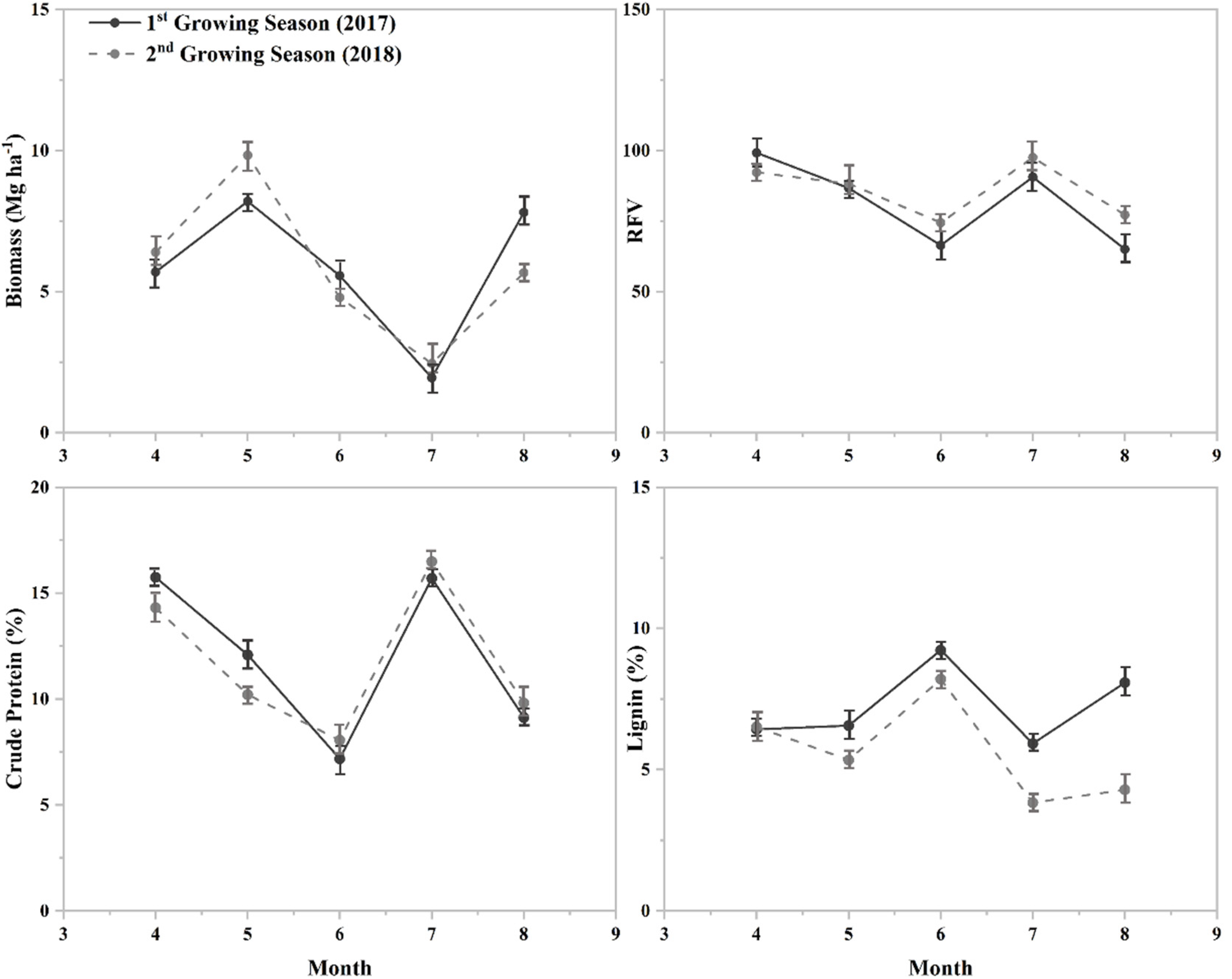
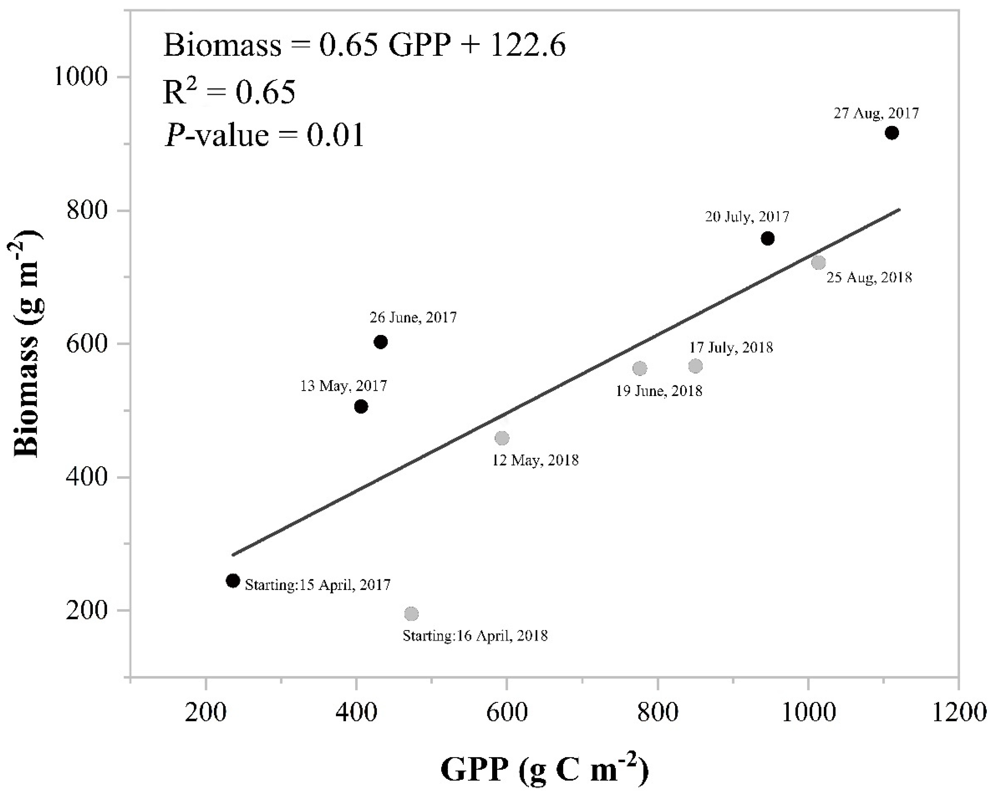
3.3. Plant Biomass and Nutritive Value

The end-of-spring season biomass production were 5.7 and 6.4 Mg ha⁻¹ in April and peaked at 8.2 and 9.8 Mg ha⁻¹ in May in the first and second growing seasons; respectively (Figure 6).

July sampling was conducted after hay cutting and, thus, resulted in very low biomass production (average: 2.2 Mg ha⁻¹). Fall-season stockpile growth increased the biomass back to 7.8 and 5.6 Mg ha⁻¹ on average for the first and second growing seasons, respectively. Grass nutritive value, indicated by RFV, was the greatest in April (average: 95.5), and started declining in the summer. The lowest values reached 66 in the first growing season. A dramatic RFV increase was detected in July immediately after each hay cutting and started declining again as biomass increased in the stockpiling season. The dynamics of grass CP level closely mirrored those of RFV. Particularly, the average late-spring and after-cutting CP level was around 15% in April and 16% in July. The low CP levels were found in June and August, averaging at 7.6 and 9.4%, respectively. Lignin concentration started low in the beginning of the growing season at 6.4% and peaked at 8.7% in June. Following hay cutting, lignin concentration dropped to 5.9 and 3.9%, in the first and second growing seasons, respectively. Overall, the cumulative above-ground biomass agreed with the cumulative GPP, yielding an R² value of 0.66 across both growing seasons (Figure 7).

3.4. Flux Data Modeling, Uncertainty Analysis, and Benchmarking

For NEE gap-filling, the overall performance of SVM-based models outcompeted all others (

Table 1. Benchmarking performance of gap-filling artificially created missing net ecosystem exchange (NEE) or latent heat flux (LE) data points. Results were evaluated as R² and root mean square error (RMSE) values (in parenthesis) based on a simple linear regression between predicted and eddy covariance-measured values. Particularly, last-square linear models (LSLM), artificial neural network (ANN), and support vector machine (SVM) algorithms were used and evaluated based on different cross validation settings (10-fold CV, 7/14 day flaking windows). Three different variable settings used by REddyProc were compared, including: global radiation, ambient air temperature, and vapor pressure deficit are all available (Rg + Tair + VPD); both Tair and VPD are missing but Rg is available (Rg); and all three variables are missing (None).

Target Variable	Algorithm	Training/Testing Partition Setting			Average
		10-Fold CV	7-Day FW	14-Day FW
NEE	LSLM	0.57 (7.8)	0.33 (17.7)	0.42 (13.9)	0.44 (13.3)
	ANN	0.64 (13.4)	0.69 (13.4)	0.02 (153.6)	0.45 (60.1)
	SVM	0.71 (12.7)	0.77 (11.8)	0.77 (11.8)	0.75 (12.1)
		Feature Setting
		None	Rg	Rg + Tair + VPD
	REddyProc	0.21 (40.9)	0.64 (15.7)	0.56 (19.6)	0.47 (25.4)
		Training/Testing Partition Setting
		10-Fold CV	7-Day FW	14-Day FW
LE	LSLM	0.61 (76.4)	0.55 (132.8)	0.57 (127.6)	0.57 (112.2)
	ANN	0.77 (105.5)	0.85 (91.7)	0.86 (87.0)	0.83 (94.7)
	SVM	0.86 (86.8)	0.90 (74.1)	0.90 (73.8)	0.89 (78.2)
		Feature Setting
		None	Rg	Rg + Tair + VPD
	REddyProc	0.79 (114.4)	0.85 (95.6)	0.87 (93.1)	0.83 (101.0)

).

The R² values of the regression between ANN-predicted NEE and the original NEE were satisfactory based on a 10-fold CV and a 7-day FW settings. However, a big reduction in performance was found when 14-day FW setting was used (R² = 0.02), which was unexpected. Meanwhile, the 7-day FW setting appeared to be a better setting compared with others. Likewise, SVM-based models yielded the optimal performance across all partition settings with an average R² value of 0.89 and an average RMSE value of 78.2. Both ANN-based models and the REddyProc software produced very similar results. The LSLM-based models generally provided the worst performance indices across all partitioning settings, and 10-fold CV generally provided the best performance for linear models. Interestingly, no performance plunge was detected under ANN-based LE models. Obviously, REddyProc gap-filling algorithms could provide reliable predictions for LE, but its performance on NEE prediction appeared to be limited. In general, the regressions between REddyProc-based predictions and original values explained more variation as more features were included in the models (from none to all three variables). Interestingly, Rg-only models appeared to be the best model (R² = 0.64) for NEE gap-filling. Finally, Figure 8 and Figure 9 depict the performance of the best gap-filling machine learning models for NEE and LE, respectively. The best results generated by REddyProc-based models were also included in both figures for comparison purposes. The optimal results of NEE and LE gap-filling were both provided by SVM-based models using 7-day FW setting.

4. Discussion

4.1. Energy Dynamics and Carbon Flux

The energy closure values obtained were generally within the range (0.6–0.9) of natural grassland ecosystems reported by other studies [24,25], which is typically lower in natural complex ecosystems such as pastures compared with row-cropping systems [26]. The remaining energy fraction can be retrieved from energy storage in the top soil layer above the heat flux plates, and from the vegetation canopy between the soil surface and the IRGA sensor head; which primarily consists converted energy by photosynthesis. The values found in this study (0.74 and 0.62 for the first and the second growing seasons, respectively) were close to the lower bound within the normal range for C3 plants [27], indicating that the EC systems properly captured and recorded energy fluxes on an ecosystem level. The slightly lower energy closure values observed in this study could be attributed to the fact that global warming gradually pushes the climate transition zones towards the north, causing significant encroachment of summer annual/perennial species (e.g., large crabgrass (Digitaria sanguinalis (L.) Scop.) purpletop, johnsongrass, dallisgrass, etc.) during late summer/early fall growing seasons. This warm-season encroachment scenario complemented the depleted production of cool-season species during hot summer months, therefore, significantly increased overall photosynthetic activity and consequentially increased biomass production and eco-efficiency. Additionally, this could also be caused by the increased heat storage portion in open canopy dominated grassland sites as reported by Wilson et al. [28].

Unlike warm-season annual/perennial grasses, which produce the majority of biomass during the late summer-early fall of each year; the growth of cool-season grasses typically peaks at the spring and fall seasons of each year with summer (summer slump) and winter dormancy periods spliced in between [29]. This bimodal growth distributions of cool-season grasses were also observed in this study (indicated by the GPP pattern in Figure 4) and are generally well-known in grassland ecosystem community. However, what is less known is the large day-by-day variation of GPP and NEE caused by different environmental and managerial factors. Particularly, hay bailing events on 17 July and 6 September 2017, as well as on 15 July 2018 rapidly transitioned the ecosystem from a net carbon sink to carbon source for a short period of time as indicated by the shifting of NEE from negative to positive numbers. Similar findings were also reported by Zhou et al. [10] from a warm-season, old world bluestem dominated grassland in Oklahoma. It was also noteworthy that GPP responded more rapidly than NEE after bailing, turning the entire ecosystem into a carbon emission source for approximately 12 days after the September cutting in 2017 and about 5 days after the July cutting in both 2017 and 2018. Additionally, the July cutting removed a small portion of senesced warm-season grasses and very little cool-season grasses that were still in summer dormancy, thus, resulting in shorter duration of responses. Following a short duration of carbon emission period, both GPP and NEE increased rapidly triggered by vigorous regrowth of young plant tissues.

The large negative daily GPP values (strong carbon sink) observed in this study were primarily caused by the warm-season grass production in summer. Additionally, greater abundance of summer-season precipitation and SVWC in the first growing season had also resulted in more negative GPP in the first growing season (Figure 1 and Figure 4). However, the first season’s NEE indicated a less carbon sink than the second season, mainly because of the increased summer respiration intensity, caused by the higher night-time temperatures associated with more precipitation (Figure 1 and Figure 4). Therefore, unlike the semiarid environment, precipitation might actually reduce carbon sequestration potential at an ecosystem level in the humid temperate regions. The seasonal cumulative GPP/NEE values obtained in this study were more negative, indicating strong biomass productivity and carbon sequestration capacity. Zhou et al. [10] also reported that GPP for a warm-season old world bluestems-based pasture only reached up to 21 g C m⁻² day⁻¹, which was very similar to those values reported by Rajan et al.) [16] and Wagle et al. [20], but only about half of what we found in our grassland ecosystem. This magnitude differences were likely caused by the fact that the majority of the warm-season grass species found in the Southeastern U.S. feature great biomass production capacity (e.g., purpletop, johnsongrass, and dallisgrass), which are well-adapted to the humid southeastern weather and typically have much larger canopy architecture than those warm-season short-bunchy grasses found in the semiarid western U.S. regions. Additionally, in an ecosystem carbon exchange comparison study, Zeri et al. [30] pointed out that the extended growing seasons of perennial warm-season grasses offer excellent carbon sequestration capacity compared to many annual species. As expected, the seasonal cumulative GPP/NEE values were substantially greater than those reported values from other managed cool-season monoculture pastures or warm-season row-cropping systems. For example, Shurpali et al. [31] reported that the annual maximum cumulative GPP of a cool-season reed canary grass (Phalaris arundinaceae L.) pasture in eastern Finland only reached −689 g C m⁻². In another study, a kentucky bluegrass monoculture pasture only yielded an annual NEE value of −1.1 kg C m⁻² [32]. Cotton et al. [33] found that a perennial warm-season hay pasture in Fort Valley of Georgia provided an annual NEE value of −1.62 kg C m⁻², which was similar to our results from the first growing season (−1.78 kg C m⁻²) but still substantially lower than the second growing season (−2.68 kg C m⁻²). In our study, we attributed the low seasonal GPP/NEE values (strong carbon sink) to the fact that the pasture was partially managed as a natural ecosystem with few biomass production gaps and almost whole-year-long growing season involving succession of dominance between cool and warm-season grass species.

Based on NEE data, the entire ecosystem remained a net carbon sink during the majority of the time within each growing season (Figure 4). This contradicts the findings reported by Skinner [9], indicating that a cool-season pasture ecosystem in Pennsylvania with very similar grass species composition could become a carbon source during the winter months. However, previous studies also indicated that transitioning from row-crop to perennial grass systems could greatly enhance GPP and NEE, but it might take more than one or two years before turning the entire ecosystem into a carbon sink [8]. The longer time period since the establishment of this pasture ecosystem might play a role in causing the differences between our study and the one reported by Skinner [16]. Meanwhile, Skinner [34] also found that the threshold temperature for C3-dominated pastures to remain actively sequestering carbon should be about −4 °C, below which is a temperature range not commonly seen in the middle Tennessee region (Figure 1). The climate transition zone of the U.S. typically has mild winter temperature and ample precipitation throughout the growing season. Therefore, the grass-dominated pasture ecosystems were rarely of a net carbon source even during the winter months.

4.2. Evapotranspiration and Ecosystem Water Use Efficiency

Information relating to quantification of ET of C3 species-dominated ecosystems is extremely limited. The EC-measured daily ET values (2.0 to 2.1 mm day⁻¹, Figure 5) obtained from this study were lower than that reported from a soybean monoculture study conducted in the Mississippi Delta region (4.4 mm day⁻¹) [27]. This is mainly caused by the differences in solar radiation intensity and solar elevation angle affected by the latitude difference. As expected, the daily ET values were smaller than that from sorghum (Sorghum bicolor L.) and maize (Zea mays L.) fields found in semiarid environments [20]. On the ecosystem level across the two growing seasons, GPP was significantly (p < 0.05) correlated with ET but the model only explained 37% of variation in the data. This indicates that the impact of precipitation/ET on carbon uptake of perennial cool-season grass dominated systems in the climate transition zones of the U.S. is moderate, as this region typically receives ample precipitation year-round. In general, C3 species have lower WUE than C4. However, summer warm-season species encroachment could significantly increase the overall EWUE. Therefore, this grassland ecosystem provided greater average EWUE (6.5 g C kg⁻¹) than that reported from warm-season perennial monoculture systems, such as old world bluestem (3.3 to 4.1 g C kg⁻¹ water); 2.5 to 3.1 g C kg⁻¹ water) [9,19] and switchgrass (3.1 g C kg⁻¹ water) [16].

4.3. Biomass Productivity and Plant Nutritive Value

The decline in plant nutritive value with advancing maturity and accumulating biomass yield was observed in this research, as indicated in other previous studies [35,36]. Summer dormancy of cool-season grasses greatly decreased the overall biomass production but this effect was largely offset by warm-season encroachment, which maintained the biomass production at above the −4.5 Mg ha⁻¹ level. Apparently, late-summer cutting significantly reduced standing biomass, and the new growth greatly increased plant nutritive value, reflected in RFV, CP, and lignin levels. The initial spring-season grass CP concentration (around 15%) largely represented the mixture of tall fescue, orchardgrass, and kentuky bluegrass; and we considered this number within the typical range of cool-season grasses without N fertilization [4]. As expected, CP concentration dropped to a very low level in summer as warm-season grasses became more abundant. Additionally, it seemed like CP was more responsive towards regrowth of juvenile tissues compared to the overall digestibility and voluntary intake responses as indicated by RFV values. In particular, RFV is a quality index that considers both NDF and ADF values, as well as their derived voluntary intake and dry matter digestibility levels [37]. Overall, the pasture ecosystem maintained RFV values between fair to utility levels.

4.4. Model Performance

The REddyProc-based gap-filling and partitioning algorithms developed and maintained by the Max Planck Institute for Biogeochemistry are widely accepted as one of the standard methods in the EC flux measurement community [22,26]. The program determines flux gaps during the low turbulent mixing values (u-star filtering) based on low friction velocity, which are identified using moving point method, breakpoint detection, or bootstrapping uncertainty analysis. The purpose for this filtering process was to remove biased flux estimates caused by undetectable advection found in the stable nocturnal surface layer below the IRGA sensor head [38]. Meanwhile, it also uses a look-up table approach based on similarities of meteorological conditions found within a 7- or 14-day time frame for gap-filling. In the original paper, Wutzler et al. [22] benchmarked their results against the BGC online tool (BGC16, 2016 version MPI-BGC in Jena Sect. 3). However, comparisons were only made between the BGC16 and REddyProc predicted values, which indicated excellent agreement; but no comparisons against EC-measured real data were performed. Therefore, we think the benchmarking results obtained from this study could be very informative to the EC flux measurement community. Additionally, Acevedo et al. [39] and Hunt et al. [6] also pointed out that the standard deviation of the vertical wind speed could serve as a better sorting parameter, but the results obtained using both were similar. Therefore, we accepted the more popular u-star-based filtering results in this study as one of the main criteria for selecting high-quality data.

The results from this study indicated that non-parametric, non-linear, kernel methods, such as SVM generally provided superior gap-filling performance than REddyProc. The ANN-based models could be used for predicting both NEE and LE gaps, but the performance stability remained questionable, which could be caused by the uncertainties associated with the structure parameters (e.g., number of hidden layers and neurons in each layer). Overall, gap-filling LE data could be completed with much greater accuracies than NEE. This is anticipated, because the carbon dynamics on an ecosystem level are governed by much more complex plant–soil–microbes interplays than LE, thus, leading to greater challenges for the modeling processes. The 10-fold CV approach used much more training data than either the 7- or 14-day FW methods. However, only one model was constructed for each routine (training and testing), consisting of nine-fold training and one-fold testing. On the other hand, both the 7- and 14-day FW methods required training and testing on each individual gap data point, thus, resulted in a much greater number of model constructions, but with substantially less training data within each routine. Overall, the 10-fold CV approach was computationally cheaper and more time-efficient. The 7- or 14-day FW methods inherently considered the time-series correlations, as only those observed data temporally close to the artificial gap data points were used for model training. Therefore, the slightly improved performance observed from the FW methods indicated that there exists some time-series correlation in the dataset but not significantly impacting the overall gap-filling performance. Finally, except for the abnormality observed under the ANN-based 14-day FW NEE gap-filling models, little difference was found between the 7- versus 14-day FW methods. This indicated that: although the threshold time length for accurate model training was unknown, a 7-day FW dataset (2 × 7 days × 48 half hours = 672 sample vectors for each training process) should contain enough information for constructing satisfactory prediction models.

To date, only a few studies have been conducted in designing and evaluating gap-filling methods for EC flux data. For example, approaches using the mean diurnal variation and the meteorological similarity-based look-up table approaches were compared by Falge et al. [40], but again, no real EC measured value-based comparisons were conducted. In another study, Hui et al. [41] constructed a multiple imputation algorithm based on expectation and maximization algorithms but the predicted results lacked consistency across various forest ecosystems. There is another ANN-based gap-filling algorithm originally proposed by Hsu et al. [42], but was largely designed for hydrological modeling not dedicated for general EC flux data. In some most recent study, Kunwor et al. [43] designed three non-linear regression approaches for gap-filling NEE, but yielded variable prediction accuracy and limited reliability. Hayek et al. [44] indicated that a simple parametric model of missing storage incorporated with a PAR-extrapolated advective respiration loss approach could yield comparable, even slightly better results for gap-filling forest NEE flux data than REddyProc. However, its applicability and effectiveness in row-crop or pasture-based ecosystem studies remain unclear. Likewise, an earlier popular EC gap-filling model developed by Dunn et al. [45] also had a strong focus on forest ecosystems. Before the advent of REddyProc, ANN-based algorithms were generally regarded as one of the best gap-filling approaches [46]. However, as indicated in this study, the uncertainties associated with its structure parameter setting and lack of stability might hinder its popularity in the future. We considered SVM as the optimal machine learning algorithm for EC gap-filling. Overall, REddyProc-based algorithms provided limited performance while predicting NEE but was relatively reliable for LE.

5. Conclusions

Taken together, a grassland pasture exemplifies a complex and dynamic ecosystem. This case study used EC tower-based flux measurement approaches, integrated with field data measurement and simulation modeling to investigate the evolution of plant phenology, nutritive value, energy balance, and carbon/water fluxes of a cool-season grassland ecosystem in the temperate climate transition region. Climate change has caused significant summer warm-season encroachment, thus, resulted in high ecoefficiency (high GPP) and EWUE. The modeling-based uncertainty analysis indicated that REddyProc can effectively predict LE data, but NEE gap filling should proceed with caution. Finally, building novel EC gap-filling models using machine learning algorithms should be important future direction.

References

1. Bond-Lamberty, B.; Thomson, A.M. Temperature-associated increases in the global soil respiration record. Nat. Cell Biol. 2010, 464, 579–582. [Google Scholar] [CrossRef] [PubMed]
2. Cumming, G.; Buerkert, A.; Hoffmann, E.M.; Schlecht, E.; Von Cramon-Taubadel, S.; Tscharntke, T. Implications of agricultural transitions and urbanization for ecosystem services. Nat. Cell Biol. 2014, 515, 50–57. [Google Scholar] [CrossRef] [PubMed]
3. Moss, R.H.; Edmonds, J.A.; Hibbard, K.A.; Manning, M.R.; Rose, S.K.; van Vuuren, D.P.; Carter, T.R.; Emori, S.; Kainuma, M.; Kram, T.; et al. The next generation of scenarios for climate change research and assessment. Nat. Cell Biol. 2010, 463, 747–756. [Google Scholar] [CrossRef] [PubMed]
4. Kallenbach, R.; Roberts, C.; Lory, J.; Hamilton, S. Nitrogen Fertilization Rates Influence Stockpiled Tall Fescue Forage through Winter. Crop Sci. 2017, 57, 1732–1741. [Google Scholar] [CrossRef]
5. Nelson, C.J.; Moore, K.J.; Collins, M. Forages and Grassland in a Changing World. In Forages, Volume 1: An Introduction to Grassland Agriculture, 7th ed.; Blackwell Publishing: Ames, IA, USA, 2018; pp. 3–18. [Google Scholar]
6. Hunt, J.E.; Laubach, J.; Barthel, M.; Fraser, A.; Phillips, R.L. Carbon budgets for an irrigated intensively grazed dairy pasture and an unirrigated winter-grazed pasture. Biogeosciences 2016, 13, 2927–2944. [Google Scholar] [CrossRef] [Green Version]
7. Leahy, P.; Kiely, G. The effect of introducing a winter forage rotation on CO2 fluxes at a temperate grassland. Agric. Ecosyst. Environ. 2012, 156, 49–56. [Google Scholar] [CrossRef] [Green Version]
8. Lohila, A. Annual CO2exchange of a peat field growing spring barley or perennial forage grass. J. Geophys. Res. Space Phys. 2004, 109, 18116. [Google Scholar] [CrossRef]
9. Skinner, H. Winter carbon dioxide fluxes in humid-temperate pastures. Agric. For. Meteorol. 2007, 144, 32–43. [Google Scholar] [CrossRef]
10. Zhou, Y.; Xiao, X.; Wagle, P.; Bajgain, R.; Mahan, H.; Basara, J.; Dong, J.; Qin, Y.; Zhang, G.; Luo, Y.; et al. Examining the short-term impacts of diverse management practices on plant phenology and carbon fluxes of Old World bluestems pasture. Agric. For. Meteorol. 2017, 237–238, 60–70. [Google Scholar] [CrossRef] [Green Version]
11. Kallenbach, R.L. Describing the Dynamic: Measuring and Assessing the Value of Plants in the Pasture. Crop Sci. 2015, 55, 2531–2539. [Google Scholar] [CrossRef]
12. Bates, G.; Harper, C.; Allen, F. Forage & Field Crop Seeding Guide For Tennessee. The University of Tennessee Agricultural Extension Service, PB378 8/08 E12-5115-00-004-09 09-0041, 2008. Available online: http://trace.tennessee.edu/utk_agexcrop/41 (accessed on 12 July 2021).
13. Reichstein, M.; Falge, E.; Baldocchi, D.; Papale, D.; Aubinet, M.; Berbigier, P.; Bernhofer, C.; Buchmann, N.; Gilmanov, T.; Granier, A.; et al. On the separation of net ecosystem exchange into assimilation and ecosystem respiration: Review and improved algorithm. Glob. Chang. Biol. 2005, 11, 1424–1439. [Google Scholar] [CrossRef]
14. Papale, D.; Reichstein, M.; Aubinet, M.; Canfora, E.; Bernhofer, C.; Kutsch, W.; Longdoz, B.; Rambal, S.; Valentini, R.; Vesala, T.; et al. Towards a standardized processing of Net Ecosystem Exchange measured with eddy covariance technique: Algorithms and uncertainty estimation. Biogeosciences 2006, 3, 571–583. [Google Scholar] [CrossRef] [Green Version]
15. Falge, E.; Baldocchi, D.; Olson, R.; Anthoni, P.; Aubinet, M.; Bernhofer, C.; Burba, G.; Ceulemans, R.J.; Clement, R.; Dolman, A.; et al. Gap filling strategies for defensible annual sums of net ecosystem exchange. Agric. For. Meteorol. 2001, 107, 43–69. [Google Scholar] [CrossRef] [Green Version]
16. Abraha, M.; Gelfand, I.; Hamilton, S.K.; Shao, C.; Su, Y.-J.; Robertson, G.P.; Chen, J. Ecosystem Water-Use Efficiency of Annual Corn and Perennial Grasslands: Contributions from Land-Use History and Species Composition. Ecosystems 2016, 19, 1001–1012. [Google Scholar] [CrossRef]
17. Rajan, N.; Maas, S.J.; Cui, S. Extreme Drought Effects on Carbon Dynamics of a Semiarid Pasture. Agron. J. 2013, 105, 1749–1760. [Google Scholar] [CrossRef] [Green Version]
18. Zeeman, M.; Hiller, R.; Gilgen, A.K.; Michna, P.; Plüss, P.; Buchmann, N.; Eugster, W. Management and climate impacts on net CO2 fluxes and carbon budgets of three grasslands along an elevational gradient in Switzerland. Agric. For. Meteorol. 2010, 150, 519–530. [Google Scholar] [CrossRef] [Green Version]
19. Wagle, P.; Kakani, V.G.; Huhnke, R. Evapotranspiration and Ecosystem Water Use Efficiency of Switchgrass and High Biomass Sorghum. Agron. J. 2016, 108, 1007–1019. [Google Scholar] [CrossRef]
20. Wagle, P.; Gowda, P.H.; Moorhead, J.E.; Marek, G.W.; Brauer, D.K. Net ecosystem exchange of CO2 and H2O fluxes from irrigated grain sorghum and maize in the Texas High Plains. Sci. Total Environ. 2018, 637–638, 163–173. [Google Scholar] [CrossRef]
21. Murray, I.; Cowe, I. Sample preparation. In Near-Infrared Spec-Troscopy in Agriculture; Roberts, C.A., Workman, J.J., Reeves, J.B., Eds.; ASA, CSSA, and SSSA: Madison, WI, USA, 2004; pp. 75–112. [Google Scholar]
22. Wutzler, T.; Lucas-Moffat, A.; Migliavacca, M.; Knauer, J.; Sickel, K.; Šigut, L.; Menzer, O.; Reichstein, M. Basic and extensible post-processing of eddy covariance flux data with REddyProc. Biogeosciences 2018, 15, 5015–5030. [Google Scholar] [CrossRef] [Green Version]
23. Kljun, N.; Calanca, P.; Rotach, M.W.; Schmid, H.P. A simple two-dimensional parameterisation for Flux Footprint Prediction (FFP). Geosci. Model Dev. 2015, 8, 3695–3713. [Google Scholar] [CrossRef] [Green Version]
24. Foken, T. The Energy Balance Closure Problem: An Overview. Ecol. Appl. 2008, 18, 1351–1367. [Google Scholar] [CrossRef] [PubMed]
25. Rajan, N.; Maas, S.J.; Cui, S. Extreme drought effects on summer evapotranspiration and energy balance of a grassland in the Southern Great Plains. Ecohydrology 2015, 8, 1194–1204. [Google Scholar] [CrossRef]
26. Anapalli, S.S.; Fisher, D.K.; Reddy, K.N.; Krutz, J.L.; Pinnamaneni, S.R.; Sui, R. Quantifying water and CO2 fluxes and water use efficiencies across irrigated C3 and C4 crops in a humid climate. Sci. Total Environ. 2019, 663, 338–350. [Google Scholar] [CrossRef] [PubMed]
27. Anapalli, S.S.; Fisher, D.K.; Reddy, K.N.; Wagle, P.; Gowda, P.H.; Sui, R. Quantifying soybean evapotranspiration using an eddy covariance approach. Agric. Water Manag. 2018, 209, 228–239. [Google Scholar] [CrossRef]
28. Wilson, K.; Goldstein, A.; Falge, E.; Aubinet, M.; Baldocchi, D.; Berbigier, P.; Bernhofer, C.; Ceulemans, R.; Dolman, H.; Field, C.; et al. Energy balance closure at FLUXNET sites. Agric. For. Meteorol. 2002, 113, 223–243. [Google Scholar] [CrossRef] [Green Version]
29. Collins, M.; Nelson, C.J. Grasses for Northern Areas. In Forages, Volume 1: An Introduction to Grassland Agriculture, 7th ed.; Collins, M., Nelson, C.J., Moore, K.J., Barnes, R.F., Eds.; Blackwell Publishing: Ames, IA, USA, 2018; pp. 131–132. [Google Scholar]
30. Zeri, M.; Andersonteixeira, K.J.; Hickman, G.C.; Masters, M.D.; DeLucia, E.H.; Bernacchi, C. Carbon exchange by establishing biofuel crops in Central Illinois. Agric. Ecosyst. Environ. 2011, 144, 319–329. [Google Scholar] [CrossRef] [Green Version]
31. Shurpali, N.J.; Hyvönen, N.P.; Huttunen, J.T.; Clement, R.J.; Reichstein, M.; Nykänen, H.; Biasi, C.; Martikainen, P.J. Cultivation of a perennial grass for bioenergy on a boreal organic soil—Carbon sink or source? GCB Bioenergy 2009, 1, 35–50. [Google Scholar] [CrossRef]
32. Wu, J.; Bauer, M.E. Estimating Net Primary Production of Turfgrass in an Urban-Suburban Landscape with QuickBird Imagery. Remote Sens. 2012, 4, 849–866. [Google Scholar] [CrossRef] [Green Version]
33. Cotten, D.L.; Zhang, G.; Leclerc, M.Y.; Raymer, P.; Steketee, C.J. Carbon dioxide fluxes from Tifway bermudagrass: Early results. Int. J. Biometeorol. 2017, 61, 103–113. [Google Scholar] [CrossRef]
34. Skinner, R.H.; Adler, P.R. Carbon dioxide and water fluxes from switchgrass managed for bioenergy production. Agric. Ecosyst. Environ. 2010, 138, 257–264. [Google Scholar] [CrossRef]
35. Cui, S.; Allen, V.G.; Brown, C.P.; Wester, D.B. Growth and Nutritive Value of Three Old World Bluestems and Three Legumes in the Semiarid Texas High Plains. Crop Sci. 2013, 53, 329–340. [Google Scholar] [CrossRef]
36. Gelley, C.; Nave, R.L.G.; Bates, G. Forage Nutritive Value and Herbage Mass Relationship of Four Warm-Season Grasses. Agron. J. 2016, 108, 1603–1613. [Google Scholar] [CrossRef] [Green Version]
37. Collins, M.; Newman, Y.C. Forage quality. In Forages, Volume 1: An Introduction to Grassland Agriculture, 7th ed.; Collins, M., Nelson, C.J., Moore, K.J., Barnes, R.F., Eds.; Blackwell Publishing: Ames, IA, USA, 2018; pp. 339–354. [Google Scholar]
38. Gu, L.; Falge, E.M.; Boden, T.; Baldocchi, D.D.; Black, T.; Saleska, S.R.; Suni, T.; Verma, S.B.; Vesala, T.; Wofsy, S.C.; et al. Objective threshold determination for nighttime eddy flux filtering. Agric. For. Meteorol. 2005, 128, 179–197. [Google Scholar] [CrossRef] [Green Version]
39. Acevedo, O.C.; Moraes, O.; Degrazia, G.A.; Fitzjarrald, D.R.; Manzi, A.O.; Campos, J.G. Is friction velocity the most appropriate scale for correcting nocturnal carbon dioxide fluxes? Agric. For. Meteorol. 2009, 149, 1–10. [Google Scholar] [CrossRef]
40. Falge, E.; Baldocchi, D.; Olson, R.; Anthoni, P.; Aubinet, M.; Bernhofer, C.; Burba, G.; Ceulemans, R.; Clement, R.; Dolman, A.; et al. Gap filling strategies for long term energy flux data sets. Agric. For. Meteorol. 2001, 107, 71–77. [Google Scholar] [CrossRef] [Green Version]
41. Hui, D.; Wan, S.; Su, B.; Katul, G.; Monson, R.; Luo, Y. Gap-filling missing data in eddy covariance measurements using multiple imputation (MI) for annual estimations. Agric. For. Meteorol. 2004, 121, 93–111. [Google Scholar] [CrossRef]
42. Hsu, K.-L.; Gupta, H.; Gao, X.; Sorooshian, S.; Imam, B. Self-organizing linear output map (SOLO): An artificial neural network suitable for hydrologic modeling and analysis. Water Resour. Res. 2002, 38, 1302. [Google Scholar] [CrossRef] [Green Version]
43. Kunwor, S.; Starr, G.; Loescher, H.W.; Staudhammer, C.L. Preserving the variance in imputed eddy-covariance measurements: Alternative methods for defensible gap filling. Agric. For. Meteorol. 2017, 232, 635–649. [Google Scholar] [CrossRef] [Green Version]
44. Hayek, M.N.; Wehr, R.; Longo, M.; Hutyra, L.R.; Wiedemann, K.; Munger, J.W.; Bonal, D.; Saleska, S.R.; Fitzjarrald, D.R.; Wofsy, S.C. A novel correction for biases in forest eddy covariance carbon balance. Agric. For. Meteorol. 2018, 250–251, 90–101. [Google Scholar] [CrossRef]
45. Dunn, A.L.; Barford, C.C.; Wofsy, S.C.; Goulden, M.L.; Daube, B.C. A long-term record of carbon exchange in a boreal black spruce forest: Means, responses to interannual variability, and decadal trends. Glob. Chang. Biol. 2007, 13, 577–590. [Google Scholar] [CrossRef] [Green Version]
46. Moffat, A.M.; Papale, D.; Reichstein, M.; Hollinger, D.Y.; Richardson, A.D.; Barr, A.G.; Beckstein, C.; Braswell, B.; Churkina, G.; Desai, A.R.; et al. Comprehensive comparison of gap-filling techniques for eddy covariance net carbon fluxes. Agric. For. Meteorol. 2007, 147, 209–232. [Google Scholar] [CrossRef]
Figure 1. Daily ambient air and soil temperature (top), precipitation, and soil volumetric water content (SVWC, bottom) of a grass-dominated grassland ecosystem from the 2016–2017 and 2017–2018 growing seasons located in Middle Tennessee. Dashed lines separate years from each other.
Agronomy 11 02071 g001
Figure 2. The overall data analysis scheme and logic flow of the net ecosystem exchange (NEE) and latent heat flux (LE) gap-filling and uncertainty analysis.
Agronomy 11 02071 g002
Figure 3. Energy balance closure for the 2016–2017 and 2017–2018 growing seasons of a cool-season grass dominated grassland ecosystem located in Middle Tennessee. Rn, G, H and LE represent net radiation, soil heat flux, sensible heat flux, and latent heat flux; respectively. Data points used were based on 30 min average values.
Agronomy 11 02071 g003
Figure 4. Thirty-minute average net ecosystem exchange (NEE) and the partitioned gross primary production (GPP) and ecosystem respiration (ER) of a cool-season grass-dominated grassland ecosystem from the 2016–2017 and 2017–2018 growing seasons located in Middle Tennessee. Dashed lines separate calendar years from each other.
Agronomy 11 02071 g004
Figure 5. Daily cumulative evapotranspiration (ET) of a grass-dominated grassland ecosystem from the 2016–2017 and 2017–2018 growing seasons located in Middle Tennessee. Dashed lines separate calendar years from each other.
Agronomy 11 02071 g005
Figure 6. Evolution of biomass, relative feed value (RFV), crude protein (CP) concentration, and lignin concentration from April to August within the 2017 and 2018 growing seasons of a grass-dominated grassland ecosystem located in Middle Tennessee. A one-time hay harvest was conducted around each mid-July.
Agronomy 11 02071 g006
Figure 7. Above-ground biomass yield versus cumulative gross primary production (GPP) from April to August within the 2017 and 2018 growing seasons of a grass-dominated grassland ecosystem located in Middle Tennessee.
Agronomy 11 02071 g007
Figure 8. Benchmarking results of filling artificial gaps of the net ecosystem exchange (NEE) data based on the optimal prediction models and cross-validation settings. Regressions of predicted NEE by the REddyProc software using just global radiation alone (top-left), support vector machine (SVM, top-right) and artificial neural network (ANN, bottom-left) using 7-day window training data flanking each missing/testing value, and the least-square linear model (LSLM) based on a 10-fold cross validation (10-fold CV, bottom-right); against the eddy-covariance (EC) measured NEE values are presented. The red line indicated 1:1 perfect prediction line.
Agronomy 11 02071 g008
Figure 9. Benchmarking results of filling artificial gaps of the latent heat flux (LE) data based on the optimal prediction models and cross-validation settings. Regressions of predicted NEE by the REddyProc software using global radiation, ambient air temperature (Tair), and vapor pressure deficit (VAP, top-left); support vector machine (SVM, top-right) and artificial neural network (ANN, bottom-left) using 7- and 14-day window training data flanking each missing/testing value, respectively; and the least-square linear model (LSLM) based on a 10-fold cross validation (10-fold CV, bottom-right); against the eddy-covariance (EC) measured LE values are presented. The red line indicated 1:1 perfect prediction line.
Agronomy 11 02071 g009