Predicting the Emergence of Echinochloa crus-galli (L.) P. Beauv. in Maize Crop in Croatia with Hydrothermal Model

Abstract

Echinochloa crus-galli (L.) P. Beauv. is the most common monocotyledonous weed in maize crops in Croatia. Crop–weed interference is influenced by weed emergence patterns, and knowledge of the timing of weed emergence is crucial for the development of an efficient integrated weed-management program. Therefore, two-year field experiments were conducted in a maize crop sown in early May in continental Croatia to determine the emergence pattern of E. crus-galli from natural seedbank. In laboratory studies, the estimated base temperature and base water potential for the Croatian ecotype of E. crus-galli were 10.8 °C and −0.97 MPa, respectively. Then, the estimated germination parameters were compared with the values embedded in the AlertInf model from Italy (Veneto) to calibrate this hydrothermal model. The estimated hydrothermal units were around 28 for the onset (10%) and 93 for the middle (50%) emergence of E. crus-galli. Our findings showed that the AlertInf model satisfactorily simulated the emergence of E. crus-galli in maize crop in Croatia (EF = 0.97 in 2019 and 0.98 in 2020), indicating its potential use in other geographical areas

1. Introduction

Crop-weed interference is affected by the timing of weed emergence, and knowledge of the peak weed emergence period is critical to developing an effective integrated weed-management program [1]. According to Vleeshouwers and Kropff [2], emergence is the result of two different processes: germination and pre-emergence growth. Each process is influenced by different abiotic and biotic environmental factors, which consequently determine the timing of weed emergence. Seed germination is influenced by soil temperature, soil moisture, light exposure, temperature fluctuations, nitrate concentration, soil pH, and gaseous environment in the soil [3]. After successful germination, the developed seedlings or coleoptile emerge from the soil, and the factors that can influence the pre-emergence growth and emergence are soil type, soil texture, timing of tillage, depth of tillage, type of tillage, crop residues, etc. [4]. The timing of weed emergence can be predicted using weed emergence models.

Adequate soil temperature and moisture are the main factors triggering emergence [5]; both mechanistic and empirical models include these factors. Mechanistic models are developed in growing chambers using a different range of temperatures and water potentials, while empirical models rely on the observations of the emergence in the field and the periodicity of occurrence of certain species as a function of weather data [6,7,8]. Both models describe weed emergence with hydrothermal time (HTT), which is based on two germination parameters - base temperature (T_b) and base water potential (Ψ_b). T_b is the lowest temperature at which germination can occur, while Ψ_b is the minimum value of soil water potential at optimal temperature under which the germination rate is zero [9,10]. Based on these parameters, hydrothermal units (HT) are accumulated during the growing season when the average daily soil or air temperature and soil water potential were above Ψ_b, respectively, until the end of weed emergence. HT units are growing degree day-like measurements that accumulate the heat units above T_b only on days when soil moisture is above Ψ_b.

These models have been shown to be sufficiently accurate in predicting weed emergence in specific areas where they have been developed. For example, in maize, two HTT models are available as software applications for growers: AlertInf in Italy [11] and WeedCast in the United States [12].

The idea of extending the models to other climatic zones was proposed by Grundy [1]. However, for reliable application of the predictive emergence model, the germination parameters of the local populations should be estimated. This is because the conditions specific for seed development as well as numerous other abiotic and biotic factors can influence the adaptation and behavior of the plant in a given climatic region [13]. In addition, climate change may affect weed germination behavior. Therefore, it is important to study the biology of weed germination for each population. Laboratory experiments have shown the differences in the values of the germination parameters of different populations of the same species. For example, Leiblein-Wild et al. [14] estimated the differences in T_b between European and North American populations of Ambrosia artemisiifolia L. (2.0 °C and 4.2 °C, respectively) and explained this variation as an adaptation to new agroecological conditions, which is a characteristic of invasive plant species. In addition, Bürger and Colbach [15] estimated different T_b values for Chenopodium album L. and Echinochloa crus-galli (L.) P. Beauv. between the French and German populations, with 5.8 °C vs. 1.5 °C and 6.2 °C vs. 10.2 °C, respectively. Although the data of estimated Ψ_b between populations of the same weed species are limited, Masin et al. [7] estimated different values of Ψ_b for two populations of Amaranthus retroflexus L. in Italy (Padova, Pisa). The estimated values of Ψ_b for the populations in Padova and Pisa were 0.41 MPa and −0.62 MPa, respectively. Excluding specific population germination parameters, Loddo et al. [13] attempted to validate the AlertInf model for Abutilon theophrasti Med. with populations collected at eight sites in Europe and the USA, and validation was successful at only two sites. However, model validation is more successful when calibrated for the specific geographic location. For example, Leblanc et al. [16] successfully predicted C. album emergence by calibrating the model for different soils at three sites in Canada. Additionally, Masin et al. [11] in Italy successfully transferred the AlertInf model from the Veneto to Tuscany regions for three species (C. album, Sorghum halepense (L.) Pers., and A. theophrasti) in which the estimated germination parameters were not statistically different between the two populations.

Currently, weed emergence prediction using the AlertInf model is possible for ten summer species: A. theophrasti, Digitaria sanguinalis (L.) Scop., E. crus-galli, Polygonum persicaria L., Setaria viridis (L.) Beauv., Solanum nigrum L., A. retroflexus, C. album, Setaria pumila (Poir.) Roem & Schultz, and S. halepense [7]. Among the species included in the model, E. crus-galli is by far the most interesting to test the ability to extend the prediction of its emergence in Croatia. Being one of the most problematic weeds in the world [17], it is also the important weed in maize crop in Croatia occurring in 91% of the fields on the Croatian mainland monitored over a 40-year period (1969–2009) [18]. In untreated plots in Croatian soybean field trials, this weed species was present with an average of 48 plants per square meter [19]. The population density of E. crus-galli is similar in other row crops such as maize, where the competition caused by this species reduces grain yield by up to 50%, depending on the density of E. crus-galli and the crop growth stage [20].

The successful validation and transfer of the model AlertInf from Veneto to the Tuscany region has generated the idea of possibly using the model in maize crop in Croatia. Namely, maize is the most important arable crop in Croatia, and the HTT model could be a useful tool for farmers to adjust herbicide application based on predicted field emergence. Predicting weed emergence helps determine the appropriate time to apply herbicides when the largest population of weed species is present in the field. This approach contributes to low pesticide use in agriculture, as required by new EU agricultural strategies (The EU Green Deal).

Therefore, the first objective of the study was to estimate the germination parameters (T_b and Ψ_b) of a Croatian population of E. crus-galli and then to compare them with the Italian population modeled by AlertInf. The second objective was to validate the AlertInf HTT model with the emergence data of E. crus-galli observed in a maize field in continental Croatia.

2. Materials and Methods

2.1. Laboratory Experiments—Estimation of Base Temperature and Base Water Potential

Freshly matured seeds of E. crus-galli were collected in October 2013 from the Experimental Station of the University of Zagreb Faculty of Agriculture, Sasinovecki Lug (45°50′59.6″ N 16°09′53.9″ E). The seeds were cleaned, placed in paper bags, and stored in a refrigerator (4 °C) until the start of the experiment.

The laboratory germination experiments were conducted in 2014 and performed at different temperatures and water potentials in the germination chambers. To estimate T_b, 100 seeds per three replicates were sown in Petri dishes containing distilled water and sealed with parafilm to prevent evaporation. Petri dishes with sown seeds were placed in germination chambers (W87R, KW Apparecchi Scientifici SRL, Monteriggioni, Italy) at different temperatures (8, 12, 16, 20, 24, and 28 °C) and a photoperiod of 12 h:12 h (day–night). To estimate the Ψ_b, the same number of seeds was sown in plastic containers (10 cm diameter and 7 cm high) [7]. The seeds were sown in these containers to obtain a sufficient amount of solution at each water potential throughout the experimental period. Polyethylene glycol (PEG) 6000 (Sigma-Aldrich Chemie GmbH 25322-68-3, St. Louis, MO, USA) was used to achieve different water potentials, and the solutions were prepared with eight water stress levels: 0.00 (pure distilled water), −0.05, −0.10, −0.25, −0.38, −0.50, −0.80, and −1.00 MPa [21]. The PEG 6000 solutions were prepared according to the methodology described by Michel and Kaufman [21] using the formula:

OP = (−1.18 · 10⁻²) · C − (1.18 · 10⁻⁴) · C+ (2.67 · 10⁻⁴) · C·T + (8.39 · l0⁻⁷) · C²T

(1)

where OP is the osmotic pressure, C is the PEG concentration expressed as different weights to reach different stress levels, and T is the temperature (24 °C).

Plastic containers with 50 mL of PEG solution were placed at 24 °C with a photoperiod of 12 h:12 h (day–night) in the germination chamber. Temperature was chosen according to the preliminary experiments where the germination rate of E. crus-galli was highest at 24 °C. The photoperiod used in the experiment was the same as used in the experiment of Masin et al. [7]. The light intensity in the chamber was 40–50 μmol m⁻².

The monitoring of germination was performed as described in Šoštarčić et al. [22] and Masin et al. [7]. Germination was recorded daily to analyze the germination dynamics at different temperatures and water potentials. Germination lasted between 2 and 64 days, depending on the temperature and water potential.

2.2. Field Experiments and Laboratory Analyses

2.2.1. Monitoring of E. crus-galli Emergence in Maize

During the two growing seasons of maize, the emergence of E. crus-galli was monitored at the experimental station of Sasinovecki Lug to verify the transferability of the AlertInf model. The field experiment was set in a maize crop highly infested by E. crus-galli observed in a previous year. Maize was grown under recommended agronomic practices and operations. Previous crops in rotation were winter wheat (Triticum aestivum L.) and winter barley (Hordeum vulgare L.) for maize crops grown in 2019 and 2020, respectively. After harvesting winter cereals, an experimental field was moldboard ploughed in the autumn of each year. Shallow spring-tooth harrowing in early spring (mid-March) for soil loosening was followed by seedbed preparation using a field cultivator just before sowing. Hybrid Bc 418 was sown on 8 May 2019 and 5 May 2020 at the recommended rate (75.188 seeds per ha) in rows 70 cm apart.

Monitoring of E. crus-galli emergence was carried out three times a week by placing 12 metal formed squares (0.3 × 0.3 m) between maize rows. The first seedlings to emerge (with visible true leaves) of E. crus-galli were counted and then removed by gently plucking three times a week, without additional soil rotation.

Monitoring of the emergence ended when no emergent seedlings were observed for at least two weeks after closing the maize canopy (BBCH 18-19). In both years, monitoring started after maize sowing and lasted until 30 June and 29 June in 2019 and 2020, respectively.

Average daily soil temperature and soil moisture were monitored in the field by installing a temperature data logger (HOBO UA-001-08, Onset Computer Corporation, Bourne, MA, USA) and a moisture measuring devices (ECH2O 10HS Soil Water Content sensor, Meter Group Inc., Pullman, WA, USA) at the soil depth of up 5 cm. The data on air temperature and precipitation were recorded from the university meteorological station located at the experimental field, in order to compare the meteorological conditions between the two experimental years. The air temperature, soil temperature, and precipitation during the experimental period are shown in

Table 1. Average air and soil temperature and precipitation for the Sasinovecki Lug field site, recorded during the two experimental periods. Air temperature and precipitation were provided by the university meteorological station located at the experimental field, while soil temperature was recorded with the temperature data logger (HOBO UA-001-08, Onset Computer Corporation, Bourne, MA, USA).

Experimental Period	Average Air Temperature (°C)	Average Soil Temperature (°C)	Precipitation (mm)
2019
8–31 May	13.0	15.2	54.8
1–30 June	22.6	24.9	85.6
1–5 July	22.0	22.6	12.4
2020
5–31 May	15.3	17.8	58.6
1–29 June	19.3	22.1	85.6

.

2.2.2. Soil Analysis

Before the start of the experiment, a 1 m deep soil pit was dug in order to describe, sample, and classify the soil at the site. The soil profile is a Calcaric Endogleyic Fluvisol (Aric, Siltic) with the following horizons according to IUSS Working Group WRB [23]: Ap-C-Cl [24]. From each soil horizon, along with the disturbed samples, the undisturbed samples were taken using 100 cm³ cores. In this paper, only the selected properties of the 30 cm deep topsoil (ploughed layer, i.e., Ap horizon) are presented (

Table 2. Selected properties of the analyzed topsoil (Ap horizon).

Soil Physicochemical Properties a					Soil Water Retention Properties (Vol %) b
Texture	Organic matter %	CaCO3 %	pHKCl	Bulk density g cm−3	Field capacity	Plant wilting point	Plant- available water
Silt loam [25]	2.7 [25]	7.0	7.28 [25]	1.16	44.0	20.6	23.4

^a The results for soil texture, organic matter, and pH_KCl were adapted from Pintar et al. [25]. ^b The soil field capacity (FC) was measured at 0.033 MPa, and plant wilting point (PWP) was measured at 1.5 MPa; the plant-available water (PAW) volume was calculated as PAW = FC − PWP.

).

The disturbed soil samples were air-dried and sieved through the 2 mm sieve. The soil particle size distribution was determined by the pipette method. The soil organic matter (SOM) was analyzed as humus content by wet oxidation and back titration (Tyurin method). Soil carbonates were determined volumetrically as the content of CaCO₃. Soil pH was measured electrometrically using a glass electrode. Soil bulk density was obtained gravimetrically from triplicate undisturbed samples, with the mean value reported in the paper (Table 2).

Soil water retention was analyzed from the disturbed samples using the Soilmoisture Equipment Corp. extractors by applying pressures of 0.01, 0.033, 0.625, and 1.5 MPa and then by determining the corresponding soil water contents gravimetrically. The volumetric soil water contents were calculated by multiplying the mass soil water contents with the soil bulk density (Table 2). The RETC computer program (U.S. Salinity Laboratory, USDA, ARS: Riverside, CA, USA) [26] was used to build the water retention curve of the studied soil, which was then used to obtain the water potentials that correspond to the soil water contents measured during the experiment.

2.3. Statistical Analysis

A parabolic model was used to describe the effect of temperature, while a logistic model was used to describe the effect of water potential. T_b and Ψ_b were estimated using cumulative germination data, which were presented as germination dynamics. The effect of the temperature and water potential on germination dynamics, expressed in days (t₁₀, t₅₀, and t₉₀), was analyzed using means of variance analysis (ANOVA). After a significant F-test, the LSD test for p = 0.05 was used to compare the mean values. The germination dynamics curve was generated using the logistic function in the Bioassay97 statistical program [27] to determine the initial (t₁₀), medium (t₅₀), and final (t₉₀) germination times. A linear regression, estimated using the bootstrap method [28], provided the best fit of germination rate (reciprocal of time to 50% germination) against incubation temperature or water potential. The values of T_b and Ψ_b were estimated as the intercept of the regression line with the temperature or water potential axis [7,22,29].

Then, the germination parameters of E. crus-galli were compared with the germination parameters of the Italian population. The aim of the comparison was to verify whether inserting the value of the Croatian population into the AlertInf model is necessary, which would be a model recalibration, whether statistical difference is found between the values of the Italian and Croatian populations, and whether the model can be used without recalibration. The criterion of overlap of the 95% confidence intervals estimated with the bootstrap method was used to compare the values of the germination parameters of Croatian and Italian populations of E. crus-galli as described in Šoštarčić et al. [22].

The soil temperature and soil moisture data during the experimental period in the field were used to calculate hydrothermal units (HT) according to Masin et al. [30]:

HTi = n · max (T_si − T_b, 0) + HTi-1
T_si < T_o: n = 0 if Ψ_si ≤ Ψ_b; n = 1 if Ψ_si > Ψ_b
T_si > T_o: n = 0 if Ψ_si ≤ Ψ_b + K_t (T_si − T_o); n = 1 if Ψ_si> Ψ_b + K_t (T_si − T_o)

(2)

where T_si and Ψ_si are the average daily soil temperature and water potential at a depth of 5 cm, T_b is the base temperature, Ψ_b is the base water potential, T_o is the optimal temperature for seed germination, and K_t is the slope of the relationship between Ψ_b and Tsi in the supra-optimal temperature range.

Model Validation

In order to verify the applicability of the model to maize in Croatia, the weed emergence dynamics of E. crus-galli were simulated by the Italian AlertInf model [30]. Emergence dynamics are expressed by the Gompertz function according to the following equation:

CE = 100 · exp (−a · exp [−b · HT])

(3)

where CE represents cumulative emergence, a is related to an HT lag before emergence starts, and b is related to the slope of the curve.

The simulation used the daily average values of soil temperature and soil water potential recorded in the field. The germination parameters used were the estimated T_b and Ψ_b of the Croatian population, the optimal temperature (T_o), the slope (K_t), and the Gompertz coefficients (a and b) estimated for Italian populations. The cumulated emergence percentage of both years was simulated, and the predictions were compared with the observations. The overall model performance was evaluated using root mean square error (RMSE) and modeling efficiency (EF), calculated as follows:

$$\mathrm{RMSE}=\sqrt{\frac{1}{\mathrm{n}}{\displaystyle \sum }_{\mathrm{i}=1}^{\mathrm{n}}{\left({\mathrm{P}}_{\mathrm{i}}-{\mathrm{O}}_{\mathrm{i}}\right)}^2}$$

(4)

$$\mathrm{EF}=\frac{{\displaystyle \sum _{\mathrm{i}=1}^{\mathrm{n}}{({\mathrm{O}}_{\mathrm{i}}-\overline{\mathrm{O}})}^2}-{\displaystyle \sum _{\mathrm{i}=1}^{\mathrm{n}}{({\mathrm{P}}_{\mathrm{i}}-{\mathrm{O}}_{\mathrm{i}})}^2}}{{\displaystyle \sum _{\mathrm{i}=1}^{\mathrm{n}}{({\mathrm{O}}_{\mathrm{i}}-\overline{\mathrm{O}})}^2}}$$

(5)

where P_i is the simulated value, O_i is the measured value, Ō is the mean of the measured value, and N is the number of observations.

3. Results and Discussion

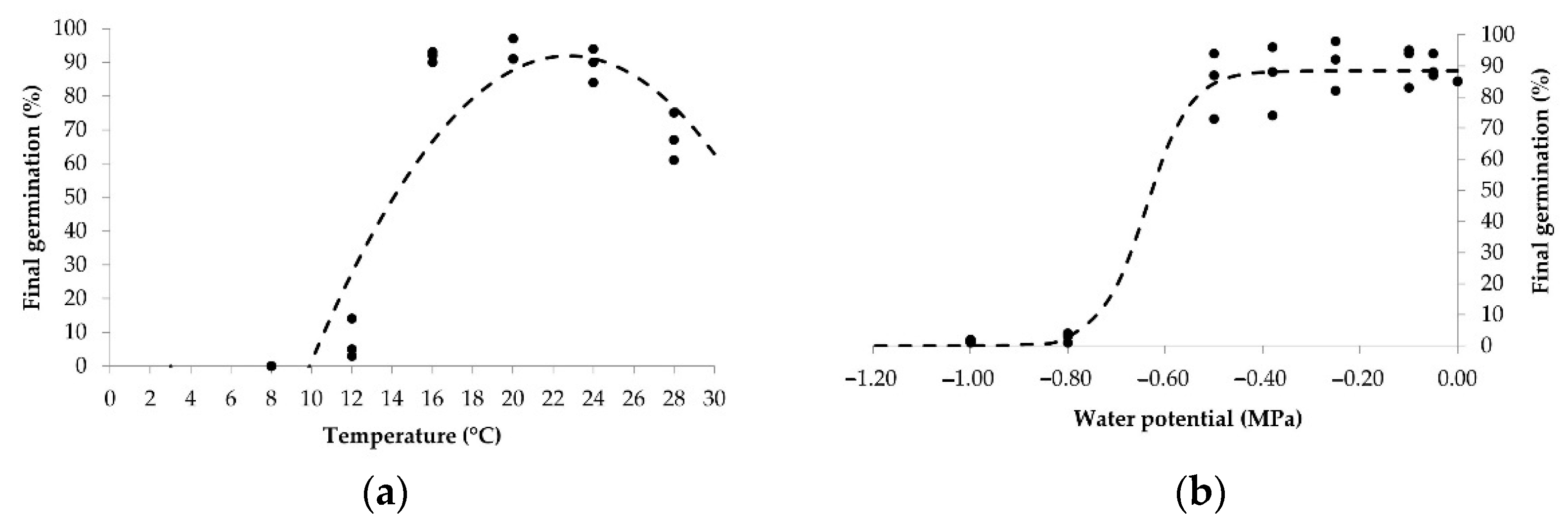
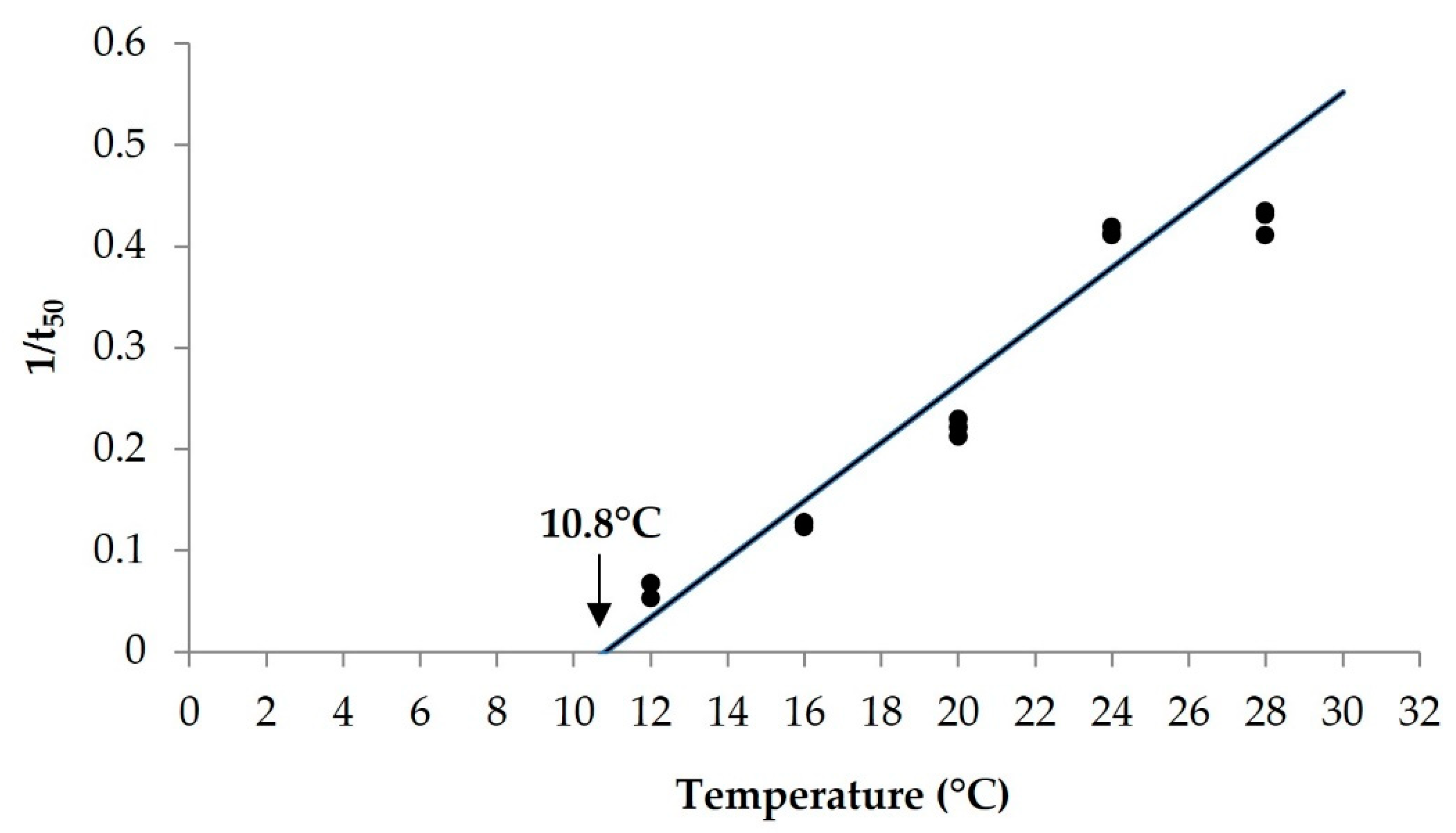
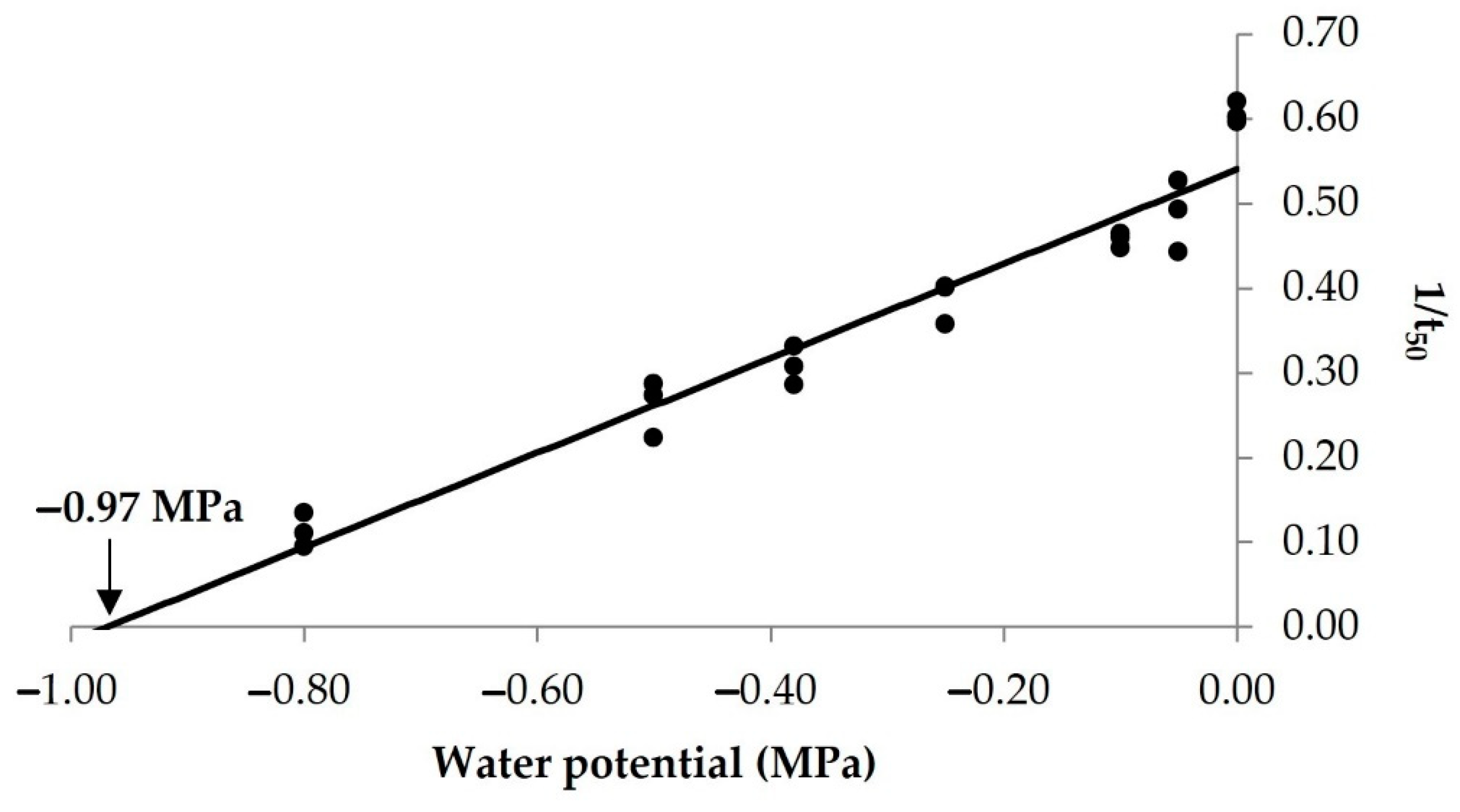
3.1. Estimation of Base Temperature and Base Water Potential

The final germination of E. crus-galli at different temperatures ranged from 0 to 93% (Figure 1a). The highest germination was recorded at temperatures 16, 20, and 24 °C (92, 93, and 89%, respectively). Germination decreased at 12 °C (7%), while no germination was recorded at 8 °C. In addition, at the highest studied temperature, 28 °C, germination decreased (68%). High germination was observed across all water potentials from 0.00 to −0.50 MPa (85–86%), and germination decreased at −0.80 MPa (3%) and −1.00 MPa (2%) (Figure 1b).

The daily recorded germination was analyzed as germination dynamics over the studied period, and the results are presented in

Table 3. Germination dynamics (t₁₀, t₅₀, and t₉₀) at the different studied temperatures and water potentials at 24 °C.

°C	t10	t50	t90	MPa	t10	t50	t90
28	1.6 a	2.4 a	3.4 a	0.00	1.3 a	1.6 a	2.1 a
24	3.2 b	3.8 ab	4.6 ab	−0.05	1.6 b	2.2 ab	3.0 a
20	3.1 b	4.6 b	6.7 b	−0.10	1.8 b	2.6 ab	3.6 a
16	5.2 e	8.1 c	12.6 c	−0.25	2.3 c	3.3 bc	4.7 a
12	13.9 d	16.2 d	18.7 d	−0.38	2.6 e	3.6 bc	4.3 a
				−0.50	2.9 d	3.9 c	5.8 a
				−0.80	1.6 b	9.0 d	50.0 b

Differences between the initial (t₁₀), medium (t₅₀), and final (t₉₀) germination under different temperatures and water potentials according to one-way analysis of variance (ANOVA). Different small letters (a–d) within a column indicate a statistical difference according to Fisher’s Least Significant Difference (LSD) test at p < 0.05.

. The germination dynamics at the different studied temperatures lasted from 3.4 to 18.7 days. As expected, the onset of germination was fastest at 28 °C, starting after 1.6 days, whereas it was the slowest at 12 °C, starting after 13.9 days. The same trend was observed for mean germination (t₅₀) and final germination (t₉₀). Germination decreased with the decrease in water potential, with statistical differences observed in t₁₀ and t₅₀. The germination dynamics were the fastest at 0.00 MPa (water-saturated environment), while taking 50 days at −0.80 MPa (dry environment).

Reciprocal time to t₅₀ was used to create a linear regression line and estimate T_b (10.8 °C, Figure 2) and Ψ_b (−0.97 MPa, Figure 3) for the Croatian population of E. crus-galli. The estimated T_b value for the Croatian population is similar to the estimated values for the Iranian population (10.4 °C) [31] and a German origin (10.2 °C) [15]. A similar value was also reported for a Texas population, 9.7 °C [32]. In contrary, the lowest T_b of E. crus-galli was estimated for a French population: 6.2 °C [33]. Meanwhile, Steinmaus [34] estimated the highest T_b, 13.8 °C, in California. To our knowledge, little information is found in the literature on the Ψ_b of E. crus-galli. However, Guillemin et al. [33] reported the Ψ_b value of −1.19 MPa for a French population.

The T_b value of the Croatian population of E. crus-galli is 0.9 °C lower than the T_b value of the Italian population (

Table 4. Comparison of base temperature (T_b) and base water potential (Ψ_b) of Echinochloa crus-galli Croatian and Italian population estimated with the bootstrap method [28], 95% confidence interval (95% CI), and coefficient of determination (r²). Estimated values of the Italian population were adapted from Masin et al. [7].

Population	Tb (°C)	±95 CI	r2	Ψb (MPa)	±95 CI	r2
Croatia	10.8	0.27	0.94	−0.97	0.06	0.94
Italy [7]	11.7	0.28	0.89	−0.97	0.04	0.95

). No overlap in the T_b values between the two populations is found; therefore, the populations differ in this parameter. However, the Ψ_b values of the two populations overlap, indicating that the Croatian and Italian populations of E. crus-galli do not differ in this parameter. Among other factors that might influence the difference in the estimated value, the climatic conditions at the two sites might have affected the T_b value. Namely, Zagreb is classified as Dfb, with a cold climate, precipitation without a dry season, and a warm summer. Padova is classified as Cfa, with a temperate climate, precipitation without a dry season, and a warm summer minimum [35]. The average annual temperature in Zagreb is 11.8 °C, while the average annual temperature in Padova is 12.2 °C. A similar trend was observed for another grass weed species, S. pumila, of which the estimated T_b of the Croatian population is 6.6 °C, while the Italian population has a T_b of 10.4 °C [22].

3.2. Field Experiments

Data on the emergence of E. crus-galli in maize crops at Sasinovecki Lug were used to validate the AlertInf model developed with germination parameters (T_b = 10.8 °C and Ψ_b = −0.97 MPa) of the Croatian population. The optimal temperature (T_o = 26 °C), the slope of the relationship (K_t = 0.1) between Ψ_b and T_si, and the Gompertz coefficient (a = 4.17, and b = 0.02) were adopted from Masin et al. [30].

As dominant weed species in a natural seedbank in a Croatian field [18], E. crus-galli was present in high density in Sasinovecki Lug. The average densities were 933 and 834 plants/m² in 2019 and 2020, respectively, which highlight the reliability of the model stimulation. Indeed, a prediction of E. crus-galli emergence by AlertInf in Veneto was performed by a much lower weed density (56.6 plants/m²) [30]. Model simulation of E. cus-galli emergence in maize at Sasinovecki Lug is shown in Figure 4a,b for 2019 and 2020, respectively. The AlertInf model fit the observed data satisfactorily, with EF indices of 0.97 and 0.98 in 2019 and 2020, respectively. However, the emergence data show that the model underestimated the onset of emergence in 2019 and overestimated it in 2020. In addition, a slight overestimation was observed in 2019 from the middle to the end of emergence. The RMSE is 1.69 and 1.38 in 2019 and 2020 respectively, which means that the average deviation predicted from measured values is small.

In 2019, the AlertInf model predicted an initial emergence (11%) of E. crus-galli at 29.1 cumulative HT units on 31 May (Figure 4a). However, in the field, this emergence was observed 5 days earlier, on 26 May, 18 days after sowing (DAS). The model predicted the middle emergence (52%) on 6 June at 96.2 cumulative HT units. Field observations at this time were similar, with emergence monitored from 4 to 8 June (40–50%). In addition, according to the model, an 81% emergence at 157.9 HT units should have occurred on 10 June. However, in the field, this was achieved on 12 June. The model predicted 91% of emergence only one day earlier than the value observed in the field (18 June vs. 19 June). Similarly, the model predicted the end of emergence (99–100%) on 26 June at 312 HT units, whereas in the field; this was on 28 June.

In contrast to 2019, in 2020, the model overestimated the onset of emergence (0–30%), while the middle and the end of emergence data were consistent with predicted values. In 2020, the onset of emergence (10%) was predicted for 16 May at 27.3 HT units (Figure 4b). In the field, this emergence was observed on 18 and 22 May, i.e., between 13 and 17 DAS. The middle emergence predicted by the model was reached at a cumulative 93.1 HT units on 24 May. The field situation was also similar, with middle emergence observed from 22 to 25 May (32–63%), i.e., 17 to 20 DAS. Moreover, the prediction of 80% of emergence was achieved at 156.3 HT units, which should have been achieved on 3 June according to the model. In the field, the 85% emergence of E. crus-galli was observed two days earlier (85%) on 1 June. The end of emergence was predicted on 17 June at 342.5 HT units, while it was observed in the field from 12 June.

As previously mentioned, the observed field emergence of E. crus-galli varied only slightly between 2019 and 2020 when calendar days were considered. In both years, emergence began after sowing (early May) and continued through the end of June, coinciding with the closing of the maize canopy and the concomitant decline in E. crus-galli emergence. The cessation of emergence with the closing of the leaf canopy has already been documented [5] and explained by the change in soil climate. However, studies based on determination of emergence pattern often are performed in a crop-free field [36,37,38]. Nevertheless, when E. crus-galli emergence was observed without the crop at 12 sites in the United States, the emergence extended into September [39]—much longer than in our study. Therefore, conducting these experiments and observing emergence within a crop and between different crops are necessary due to the differences in crop canopy architecture. [30].

Our findings suggest that the use of the AlertInf model for predicting the emergence of E. crus-galli in Sasinovecki Lug (Croatia) is fully feasible considering the threshold EF value of 0.5 for an acceptable model prediction [40]. When transferring the AlertInf from Veneto to Tuscany, Masin et al. [11] estimated the EF values for the emergence of A. theophrasti, C. album, and S. halepense to be 0.98, 0.99, and 0.98, respectively. On the contrary, Egea-Cobrero et al. [41] used the Myers et al. [42] dataset from the United Sates to validate the emergence of A. theophrasti in Golega (Portugal) and Minnesota (United States), obtaining EFs of 0.30 and 0.97, respectively. Due to the low EF in Portugal, the authors concluded that the same model could not be used in Portugal. However, the results of the current study do not allow us to generalize the application of the model to different environmental conditions and agronomic practices. For example, in this study, tillage and seedbed preparation did not differ in both years. The effect of tillage on the vertical distribution of seed in the seed bank is well known, and different tillage practices can significantly affect field emergence. However, Vasileiadis et al. [37] concluded that the emergence of E. crus-galli was stable over the years under different simulated tillage systems (conventional, reduced, and, no-till), so AlertInf could be adopted for maize grown under different tillage conditions considering this fact. Another factor that could influence the emergence and effectiveness of the model is soil type, which was not considered in this experiment and should be further investigated. A good example is the study by Leblanc et al. [16], who calibrated a predictive mathematical model to different soil types by adjusting the base temperature of C. album seedlings to the soil texture.

In order to set an appropriate time for weed control, determining the time of weed emergence in the field is important, which according to our study can be predicted for E. crus-galli by AlertInf. In Croatian maize fields, E. crus-galli is almost always controlled with pre-emergence or post-emergence herbicides, usually in combination with inter-row cultivation. According to Oriade and Forcella [43], the efficacy of inter-row cultivation is highest when 60% of S. viridis, another important monocot maize species, has emerged. Based on our experiment, inter-row cultivation should be applied from 96 to 113 cumulative HT units. The best efficacy of post-emergence foliar herbicides is achieved when 70–80% of weeds have emerged in the field [7,44]. According to AlertInf, foliar application should be made at a cumulative 140–144 HT units. Finally, the AlertInf model can be used to support the adoption of integrated weed control tactics and post-emergence band application with inter-row cultivation, which can significantly reduce herbicide use in maize [45].

4. Conclusions

E. crus-galli is the most important monocotyledonous weed in maize in Croatia and other geographical areas. The possible use of the existing weed emergence model for this species could be useful for weed control programs. In this study, the Italian AlertInf model had to be calibrated with the T_b values of the Croatian population of E. crus-galli, as there were statistical differences with the Italian population embedded in the model. The calibrated AlertInf model showed good prediction of E. crus-galli emergence when validated with field data from continental Croatia (Šašinovečki Lug). Therefore, the use of AlertInf for predicting E. crus-galli at this site is successful.

Future experiments should focus on increasing the complexity of the AlertInf model by including previously mentioned factors such as environmental conditions (soil type) and agronomic practices (type of tillage) that could influence the emergence of E. crus-galli. For practical purposes, the use of AlertInf by Croatian farmers could be a good way to predict the emergence of E. crus-galli without the need to measure and monitor all of the parameters required as inputs by complex mechanistic models [1,17]. The results of this study encourage us to extend AlertInf to other important maize weed species for which the germination parameters have already been estimated [22]. The possible extension of AlertInf to other geographical areas could be the focus of further experiments.

References

1. Grundy, A.C. Predicting weed emergence: A review of approaches and future challenges. Weed Res. 2003, 43, 1–11. [Google Scholar] [CrossRef]
2. Vleeshouwers, L.M.; Kropff, M.J. Modelling field emergence patterns in arable weeds. New Phytologist. 2000, 148, 445–457. [Google Scholar] [CrossRef]
3. Merfield, C.N. False and Stale Seedbeds: The Most Effective Non-Chemical WeedManagement Tools for Cropping and Pasture Establishment; The BHU Future Farming Centre: Lincoln, New Zealand, 2013; p. 23. [Google Scholar]
4. Mohler, C.L. Weed life history: Identifying vulnerabilities. In Ecological Management of Agricultural Weeds; Liebman, M., Mohler, C.L., Staver, C.P., Eds.; Cambridge University Press: Cambridge, UK, 2001; pp. 40–98. [Google Scholar] [CrossRef]
5. Forcella, F.; Benech-Arnold, R.L.; Sanchez, R.; Ghersa, C.M. Modeling seedling emergence. Field Crop Res. 2000, 67, 123–139. [Google Scholar] [CrossRef]
6. García, A.L.; Recasens, J.; Forcella, F.; Torra, J.; Royo-Esnal, A. Hydrothermal Emergence Model for Ripgut Brome (Bromus diandrus). Weed Sci. 2013, 61, 146–153. [Google Scholar] [CrossRef]
7. Masin, R.; Loddo, D.; Benvenuti, S.; Zuin, M.C.; Macchia, M.; Zanin, G. Temperature and Water Potential as Parameters for Modeling Weed Emergence in Central-Northern Italy. Weed Sci. 2010, 58, 216–222. [Google Scholar] [CrossRef]
8. Leguizamon, E.S.; Fernandez-Quintanilla, C.; Barroso, J.; Gonzalez-Andujar, J.L. Using thermal and hydrothermal time to model seedling emergence of Avena sterilis spp. ludoviciana in Spain. Weed Res. 2005, 45, 149–156. [Google Scholar] [CrossRef]
9. Gummerson, R.J. The effect of constant temperatures and osmotic potentials on the germination of sugar beet. J. Exp. Bot. 1986, 37, 729–741. [Google Scholar] [CrossRef]
10. Bradford, K.J. Water relations in seed germination6. In Seed Development and Germination; Kigel, J., Galili, G., Eds.; Marcel Dekker, Inc.: New York, NY, USA, 1995; pp. 351–396. [Google Scholar]
11. Masin, R.; Loddo, D.; Benvenuti, S.; Otto, S.; Zanin, G. Modeling Weed Emergence in Italian Maize Fields. Weed Sci. 2012, 60, 254–259. [Google Scholar] [CrossRef] [Green Version]
12. Archer, D.W.; Forcella, F.; Eklund, J.J.; Gunsolus, J. WeedCast Version 2.0. 2001. Available online: http://www.morris.ars.usda.gov (accessed on 15 July 2021).
13. Loddo, D.; Bozic, D.; Calha, I.M.; Dorado, J.; Izquierdo, J.; Šćepanović, M.; Barić, K.; Carlesi, S.; Leskovsek, R.; Peterson, D.; et al. Variability in seedling emergence for European and North American populations of Abutilon theophrasti. Weed Res. 2019, 59, 15–27. [Google Scholar] [CrossRef] [Green Version]
14. Leiblein-Wild, M.C.; Kaviani, R.; Tackenberg, O. Germination and seedling frost tolerance differ between the native and invasive range in common ragweed. Oecologia 2014, 174, 739–750. [Google Scholar] [CrossRef] [Green Version]
15. Bürger, J.; Colbach, N. Germination base temperature and relative growth rate of 13 weed species—Comparing populations from two geographical origins. In Proceedings of the 28th German Conference on Weed Biology and Weed Control, Braunschweig, Germany, 27 February–1 March 2018; Volume 458, pp. 419–426. [Google Scholar] [CrossRef]
16. Leblanc, M.L.; Cloutier, D.C.; Stewart, K.A.; Hamel, C. Calibration and validation of a common lambsquarters (Chenopodium album) seedling emergence model. Weed Sci. 2004, 52, 61–66. [Google Scholar] [CrossRef]
17. Holm, L.; Doll, J.; Holm, E.; Pancho, J.; Herberger, J. World Weeds: Natural Histories and Distribution; John Wiley & Sons: New York, NY, USA, 1997. [Google Scholar]
18. Šarić, T.; Ostojić, Z.; Stefanović, L.; Deneva Milanova, S.; Kazinczi, G.; Tyšer, L. The changes of the composition of weed flora in southeastern and central europe as affected by cropping practices. Herbologia 2011, 12, 8–12. [Google Scholar]
19. Šćepanović, M.; Ostojić, Z.; Barić, K. Ograničenja mogućnosti suzbijanja korova u soji nakon nicanja. In Zbornik Sažetaka 56; seminara biljne zaštite. Cvjetković, B. (ur.); Hrvatsko društvo biljne zaštite: Opatija, Croatia, 2012; pp. 27–28. [Google Scholar]
20. Bosnic, A.C.; Swanton, C.J. Influence of barnyardgrass (Echinochloa crus-galli) time of emergence and density on corn (Zea mays). Weed Sci. 1997, 45, 276–282. [Google Scholar] [CrossRef]
21. Michel, B.E.; Kaufmann, M.R. The Osmotic Potential of Polyethylene Glycol 6000. Plant Physiol. 1973, 51, 914–916. [Google Scholar] [CrossRef] [PubMed]
22. Šoštarčić, V.; Masin, R.; Loddo, D.; Brijačak, E.; Šćepanović, M. Germination parameters of selected summer weeds: Transferring of the Alertinf model to other geographical regions. Agronomy 2021, 11, 292. [Google Scholar] [CrossRef]
23. IUSS Working Group WRB. World Reference Base for Soil Resources. International Soil Classification System for Naming Soils and Creating Legends for Soil Maps; World Soil Resources Reports; No. 106; FAO: Rome, Italy, 2014. [Google Scholar]
24. FAO. Guidelines for Soil Description, 4th ed.; Food and Agriculture Organization of the United Nations: Rome, Italy, 2006; p. 97. [Google Scholar]
25. Pintar, A.; Stipičević, S.; Lakić, J.; Barić, K. Phytotoxicity of mesotrione residues on sugar beet (Beta vulgaris L.) in agricultural soils differing in adsorption affinity. Sugar Tech. 2020, 22, 137–142. [Google Scholar] [CrossRef]
26. van Genuchten, M.T.; Leij, F.J.; Yates, S.R. The RETC Code for Quantifying the Hydraulic Functions of Unsaturated Soils, Version 1.0; EPA Report 600/2-91/065; U.S. Salinity Laboratory, USDA, ARS: Riverside, CA, USA, 1991.
27. Onofri, A. Bioassay97: A new Excel VBA macro to perform statistical analyses on herbicide dose-response data. Ital. J. Agrometeorol. 2001, 3, 40–45. [Google Scholar]
28. Efron, B. Bootstrap methods: Another look at the jackknife. Ann. Stat. 1979, 7, 1–26. [Google Scholar] [CrossRef]
29. Masin, R.; Zuin, M.C.; Zanin, G.; Tridello, G. Weed Turf: Software for improving summer annual weed control in turf. Ital. J. Agrometeorol. 2005, 50, 46–50. [Google Scholar]
30. Masin, R.; Loddo, D.; Gasparini, V.; Otto, S.; Zanin, G. Evaluation of Weed Emergence Model AlertInf for Maize in Soybean. Weed Sci. 2014, 62, 360–369. [Google Scholar] [CrossRef]
31. Loddo, D.; Ghaderi-Far, F.; Rastegar, Z.; Masin, R. Base temperatures for germination of selected weed species in Iran. Plant Prot. Sci. 2018, 54, 60–66. [Google Scholar] [CrossRef] [Green Version]
32. Wiese, A.M.; Binning, L.K. Calculating the Threshold Temperature of Development for Weeds. Weed Sci. 1987, 35, 177–179. [Google Scholar] [CrossRef]
33. Guillemin, J.P.; Gardarin, A.; Granger, S.; Reibel, C.; Munier-Jolain, N.; Colbach, N. Assessing potential germination period of weeds with base temperatures and base water potentials. Weed Res. 2013, 53, 76–87. [Google Scholar] [CrossRef]
34. Steinmaus, S.J.; Prather, T.S.; Holt, J.S. Estimation of base temperatures for nine weed species. J. Exp. Bot. 2000, 51, 275–286. [Google Scholar] [CrossRef] [Green Version]
35. Kottek, M.; Grieser, J.; Beck, C.; Rudolf, B.; Rubel, F. World map of the Koppen-Geiger climate classification updated. Meteorol. Z. 2006, 15, 259–263. [Google Scholar] [CrossRef]
36. Zambrano-Navea, C.; Bastida, F.; Gonzalez-Andujar, J.L. A hydrothermal seedling emergence model for Conyza bonariensis. Weed Res. 2013, 53, 213–220. [Google Scholar] [CrossRef] [Green Version]
37. Vasileiadis, V.P.; Froud-Williams, R.J.; Loddo, D.; Eleftherohorinos, I.G. Emergence dynamics of barnyardgrass and jimsonweed from two depths when switching from conventional to reduced and no-till conditions. Span. J. Agric. 2016, 14, e1002. [Google Scholar] [CrossRef] [Green Version]
38. Werle, R.; Sandell, L.D.; Buhler, D.D.; Hartzler, R.G.; Lindquist, J.L. Predicting emergence of 23 summer annual weed species. Weed Sci. 2014, 62, 267–279. [Google Scholar] [CrossRef]
39. Bagavathiannan, M.V.; Norsworthy, J.K.; Smith, K.L.; Burgos, N. Seedbank Size and Emergence Pattern of Barnyardgrass (Echinochloa crusgalli) in Arkansas. Weed Sci. 2011, 59, 359–365. [Google Scholar] [CrossRef]
40. Ramanarayanan, T.S.; Williams, J.R.; Dugas, W.A.; Hauck, L.M.; McFarland, A.M.S. Using APEX to Identify Alternative Practices for Animal Waste Management. Part I: Model Description and Validation; ASAE Paper No. 972209; American Society of Agricultural Engineers: St. Joseph, MI, USA, 1997. [Google Scholar]
41. Egea-Cobrero, V.; Bradley, K.; Calha, I.M.; Davis, A.S.; Dorado, J.; Forcella, F.; Lindquist, J.L.; Sprague, C.L.; Gonzalez-Andujar, J.L. Validation of predictive empirical weed emergence models of Abutilon theophrasti Medik based on intercontinental data. Weed Res. 2020, 60, 297–302. [Google Scholar] [CrossRef]
42. Myers, M.W.; Curran, W.S.; VanGessel, M.J.; Calvin, D.D.; Mortensen, D.A.; Majek, B.A. Predicting weed emergence for eight annual species in the northeastern United States. Weed Sci. 2004, 52, 913–919. [Google Scholar] [CrossRef]
43. Oriade, C.; Forcella, F. Maximizing efficacy and economics of mechanical weed control in row crops through forecasts of weed emergence. J. Crop Prod. 1999, 2, 189–205. [Google Scholar] [CrossRef]
44. Otto, S.; Masin, R.; Casari, G.; Zanin, G. Weed–Corn Competition Parameters in Late-Winter Sowing in Northern Italy. Weed Sci. 2009, 57, 194–201. [Google Scholar] [CrossRef]
45. Loddo, D.; Scarabel, L.; Sattin, M.; Pederzoli, A.; Morsiani, C.; Canestrale, R.; Tommasini, M.G. Combination of herbicide band application and inter-row cultivation provides sustainable weed control in maize. Agronomy 2020, 10, 20. [Google Scholar] [CrossRef] [Green Version]
Figure 1. Estimated models of the final germination of Echinochloa crus-galli. A parabolic model was used to describe the effect of temperature (a), while a logistic model was used to describe the effect of water potential (b). The black dots represent the observed germination, while the dashed line represents the model.
Agronomy 11 02072 g001
Figure 2. Estimated base temperatures (Tb) for the germination of Echinochloa crus-galli. The solid line represents the linear regression line, and the points represent the inverse value of the time necessary to reach 50% of germination (1/t50) estimated for the single replicates. The estimated value of the base temperature is the intersection of the regression line with the X-axis, Tb = 10.8 ± 0.27; y = 0.0288x − 0.3119, and R2 = 0.94.
Agronomy 11 02072 g002
Figure 3. Estimated base water potentials (Ψb) for the germination of Echinochloa crus-galli. The solid line represents the linear regression line, and the points represent the inverse value of the time necessary to reach 50% of germination (1/t50) estimated for the single replicates. The estimated value of the base water potential is the intersection of the regression line with the X-axis, Ψb = −0.97 ± 0.06; y = 0.5578x + 0.5404, and R2 = 0.94.
Agronomy 11 02072 g003
Figure 4. Cumulative emergence of Echinochloa crus-galli observed in the field (triangle) during 2019 (a) and 2020 (b) and the AlertInf prediction of emergence (line). Hydrothermal units are expressed as calendar days. The seed bed preparation was performed on 8 May 2019 and 5 May 2020.
Agronomy 11 02072 g004aAgronomy 11 02072 g004b