Plum Ripeness Analysis in Real Environments Using Deep Learning with Convolutional Neural Networks

Abstract

Digitization and technological transformation in agriculture is no longer something of the future, but of the present. Many crops are being managed by using sophisticated sensors that allow farmers to know the status of their crops at all times. This modernization of crops also allows for better quality harvests as well as significant cost savings. In this study, we present a tool based on Deep Learning that allows us to analyse different varieties of plums using image analysis to identify the variety and its ripeness status. The novelty of the system is the conditions in which the designed algorithm can work. An uncontrolled photographic acquisition method has been implemented. The user can take a photograph with any device, smartphone, camera, etc., directly in the field, regardless of light conditions, focus, etc. The robustness of the system presented allows us to differentiate, with 92.83% effectiveness, three varieties of plums through images taken directly in the field and values above 94% when the ripening stage of each variety is analyzed independently. We have worked with three varieties of plums, Red Beaut, Black Diamond and Angeleno, with different ripening cycles. This has allowed us to obtain a robust classification system that will allow users to differentiate between these varieties and subsequently determine the ripening stage of the particular variety.

1. Introduction

Extremadura is a region in Spain with the highest agricultural potential and one of the largest exporters of raw materials in the field of agriculture. Our region is characterized by its exports, among others, of fruits such as plums. In the European Union as a whole, Spain is considered to be one of the largest producers of plums. In recent years, the volume of tonnes produced has been growing, most of which is destined for export, thus creating an strong foreign market. According to the the United Nations Food and Agriculture Organization (FAO), production in Spain in 2019 reached 179,840 tonnes of plums, making it one of the top 13 producing countries in the world. Extremadura, with 4885 ha of area in production, in 2018 is the leading national producer, with more than 74,000 tonnes. In Extremadura, growing conditions are particularly favourable, allowing long production periods from June to September, with a range of varieties of different characteristics.

The consumption of fruit and vegetables, both on the domestic and foreign markets, increasingly demands strict quality parameters, as well as the objective of preserving fresh produce on the market for a longer period of time. This makes it necessary to provide technicians and growers with the necessary knowledge to ensure that their products are of the highest possible quality and to predict certain characteristics of the fruit at an early stage, as well as the most likely harvesting date. These predictions will allow growers to adopt corrective agronomic measures, if necessary, and to know the characteristics of their harvest and, therefore, adapt to market demand. The optimum state of commercial ripeness at harvest will be key to achieving an appetising product after transport and storage until it reaches its destination. This information would be fundamental for the organisation of the campaign, which is very complex.

Currently, a great part of fruit evaluation in the field is conducted by visual inspection techniques in combination with destructive measuring equipment, which not only takes time away from production, but also consumes valuable technician time that is sometimes not available, which has great limitations. This traditional method depends on the experience and criteria of the person carrying out the evaluation. There are many varieties of plums, each with a different ripening cycle and different external characteristics. Having a model that allows us to know the state of ripening and/or growth of the fruit would allow us to adjust agronomic practices, such as irrigation, adapted to the varieties, thus optimising water consumption. It seems reasonable that with the technology currently available, systems should be implemented which, supported by image analysis and computer processing, facilitate decision making by using the available information captured quickly, automatically and reliably. Therefore, these processes should now be supported by computer tools that allow farmers to make a decision to improve production, based on artificial intelligence.

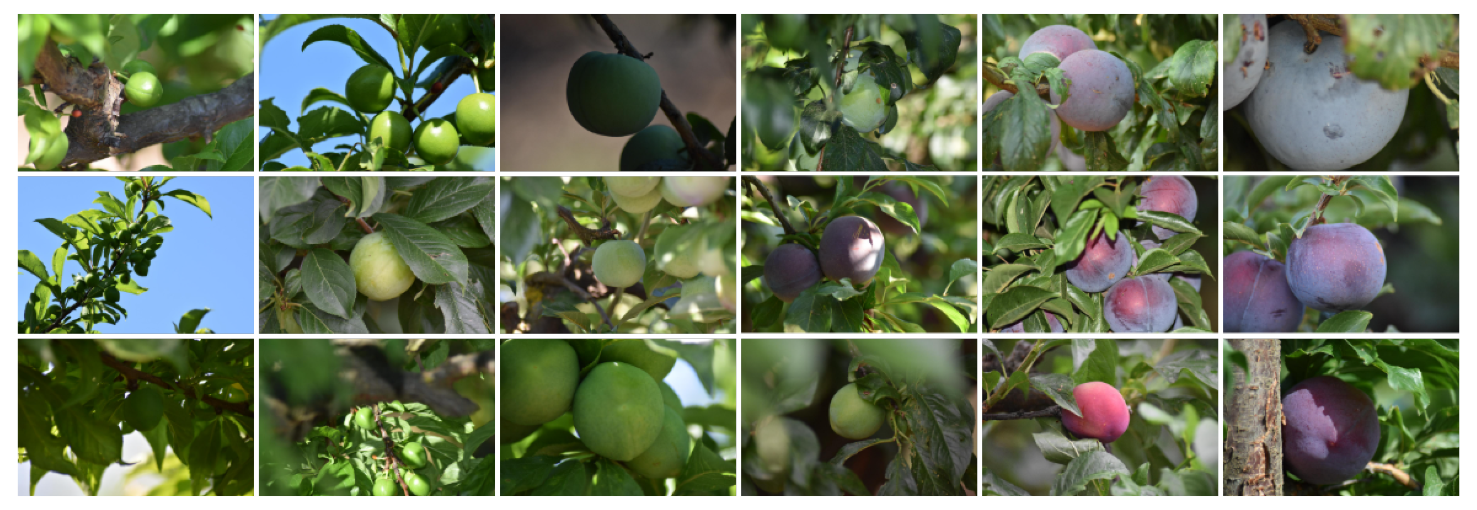
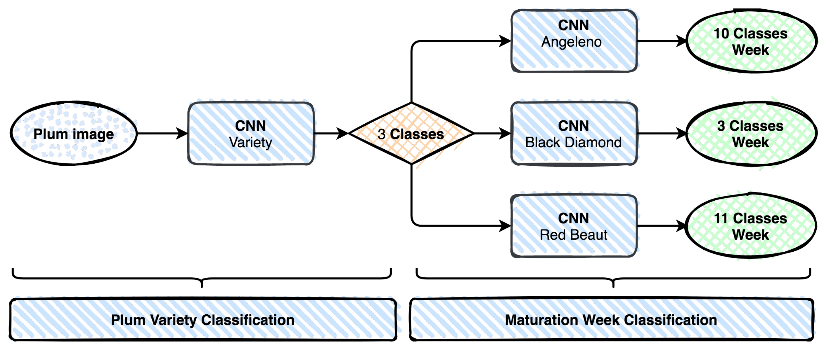
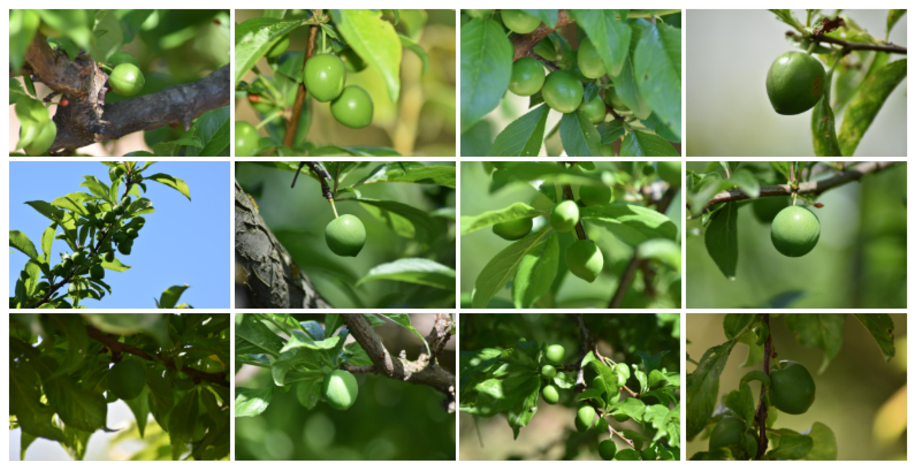
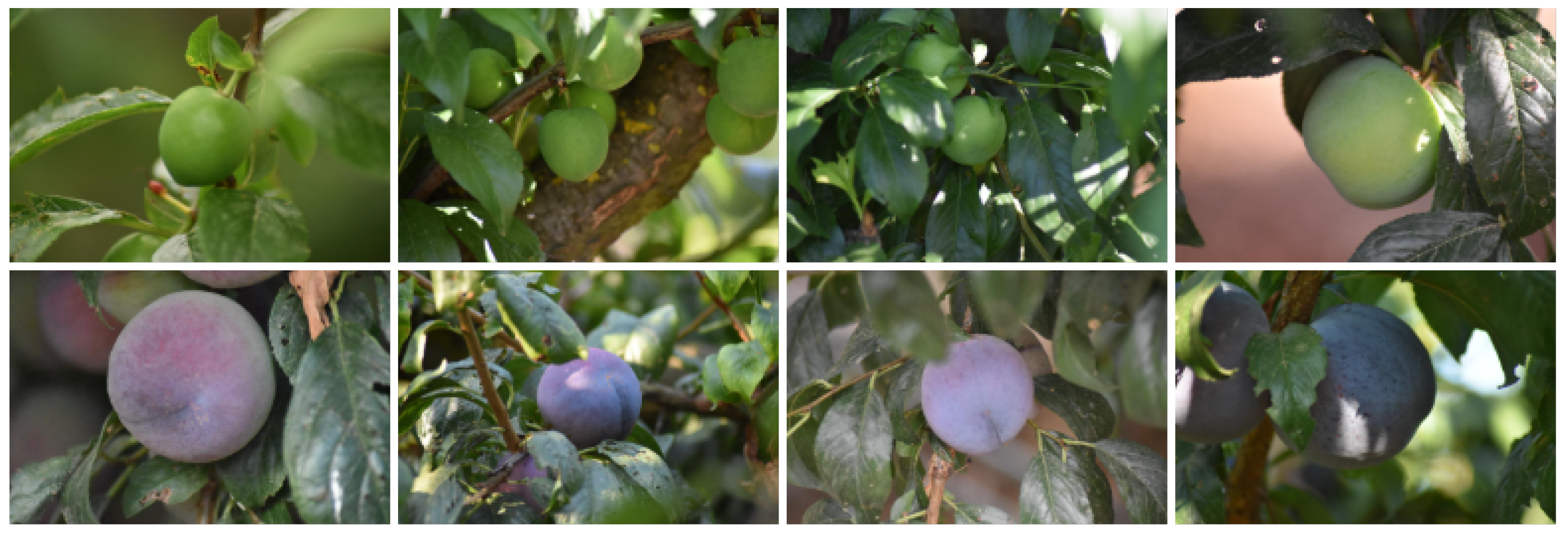
The study presented in this paper is foccused on three plum varieties, Red Beaut, Black Diamond and Angeleno, present at the Agrarian Research Center La Orden-Valdesequera (CICYTEX, Center for Scientific and Technological Research of Extremadura) (http://cicytex.juntaex.es/es/centros/la-orden-valdesequera, accessed on 17 November 2021). The main objective of this study is to identify the variety of the plums by means of an image captured by a conventional photo camera in order to subsequently detect the state of ripeness of the plum. We can focus this problem as a typical image classification problem with some peculiarities. The problem can be divided into two different sub-problems, both based on image recognition and classification: recognising the variety of plum in an image and, subsequently, recognising the ripening state of the plum. Each variety has its own ripening cycle, which implies that the study of ripening must be conducted independently for each of the varieties used in this study. We can observe two independent problems or we can build a chain of two recognition systems where we have to previously recognise the variety in order to estimate ripening. In order to understand the high difficulty level of this combined task, it is very important to highlight the nature of the images; they have been acquired in the field and in its natural environment. Unlike the images collected in a laboratory, these images have no position or illumination control, and they have different backgrounds: Sometimes there are shadows or high brights, and at many times there are partial occlusions, different zoom sizes and multiple fruits in the same picture. All of these image features turn the recognition and classification process into a more complex and more difficult achievement. 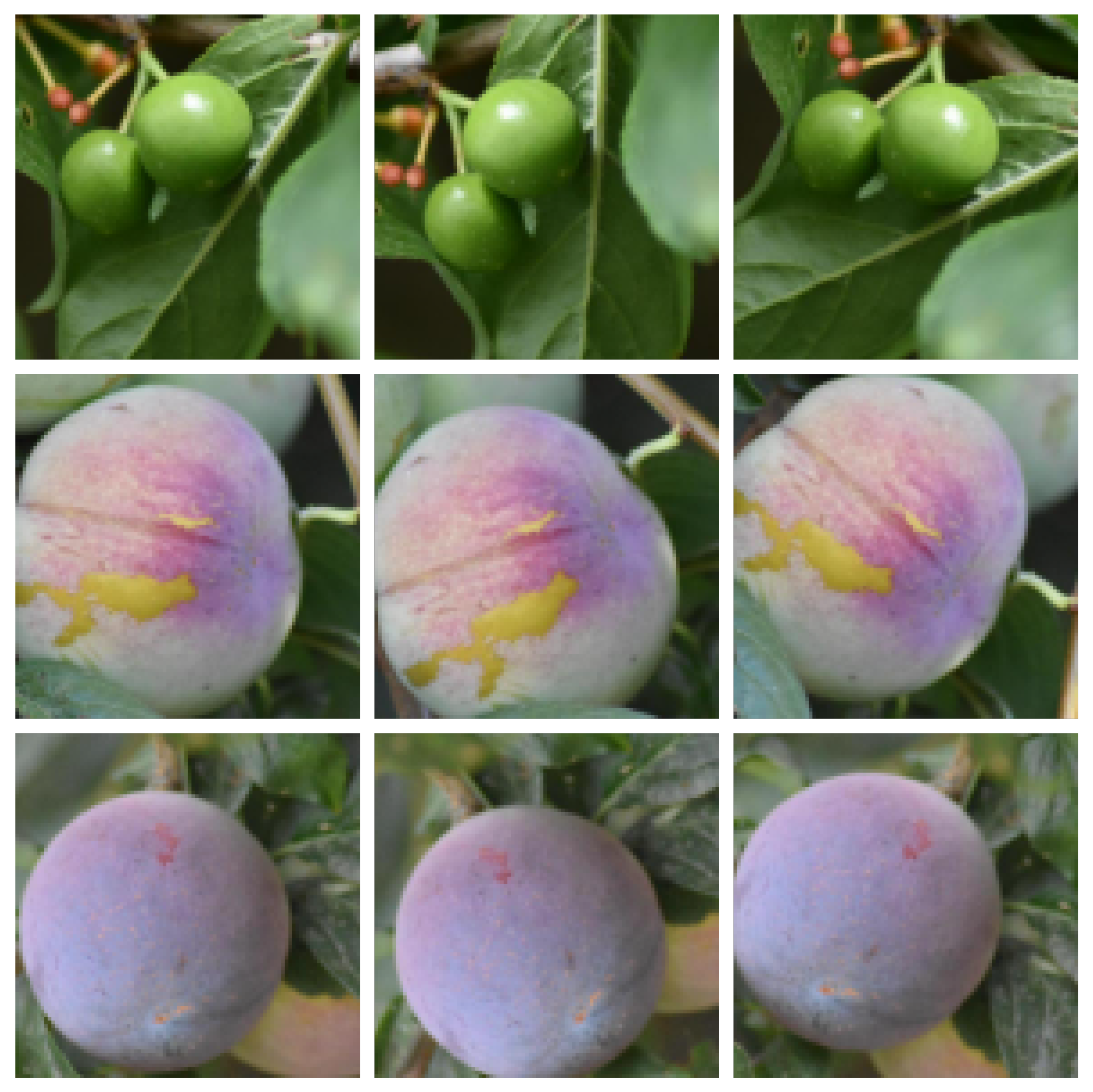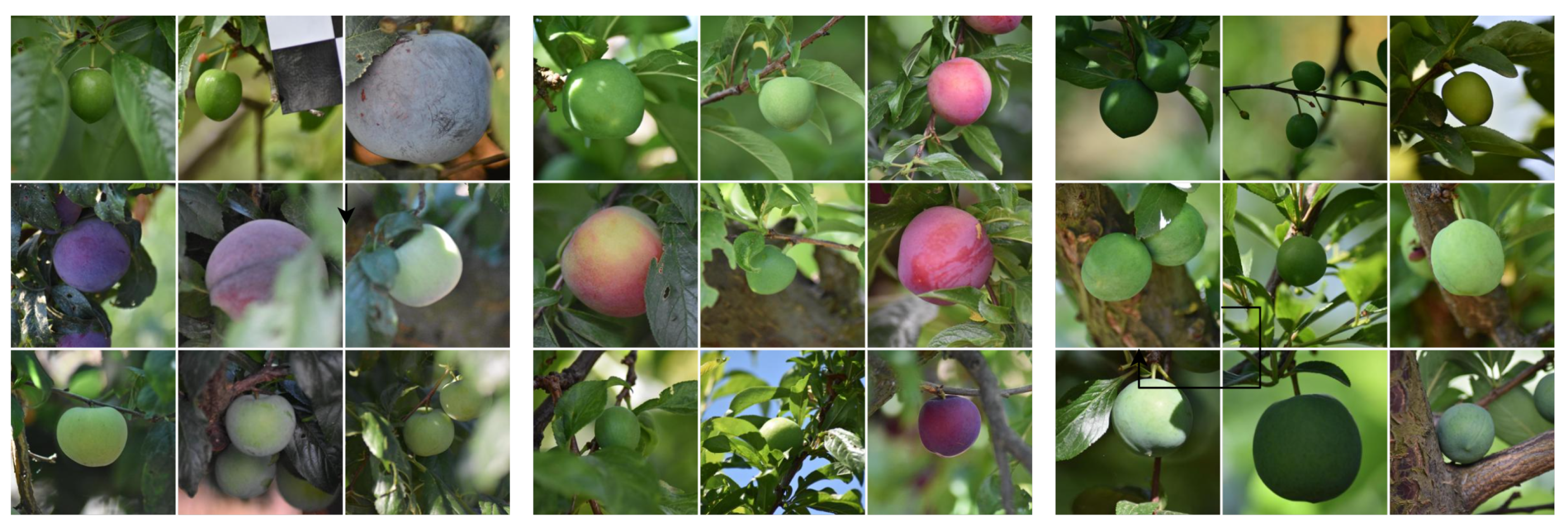In Figure 1, we can observe examples of plum images and the natural conditions of their acquisition process. The images are organized into a matrix, where each row illustrates one variety and its ripening cycle. The image classification challenges are deeply related with the image diversity along the same variety and the image similarities between different varieties. The three varieties are very similar in early stages, and they become more diverse in advanced ripeness stages, particularly in color; the shape remains similar for untrained eyes.

In the last few years, a new area of study known as deep learning (DL) has emerged in the field of machine learning. This new area encompasses different techniques that are fundamentally characterized by a hierarchical learning process in which high-level structures are automatically built starting from low-level ones across multiple layers, starting from the raw data (i.e., the pixel values of an image). DL appears as an alternative to traditional machine learning methods, which require a careful selection of hand-designed features from which the classifier can detect patterns by means of one, two at most, nonlinear transformation of those features. These classical methods have proven to be quite effective for solving simple or well-delimited problems but encounter difficulties in dealing with real-world complex problems such as object and speech recognition. By contrast, DL techniques have hugely improved the state of the art in such complex tasks. In this study, we focus on a DL technique for supervised learning known as deep convolutional neural networks (CNN) [1,2], which has shown outstanding performances for visual objects recognition. CNN benefits from the spatial structure of input data, that is, the images.

We propose a two-stage system based on DL with Convolutional Neural Networks (CNN). Among all the architectures available for CNNs applied to image classification, we used AlexNet, which has already proved is efficiency in this kind of problem [3]. Our system will address distinct problems using the same input images: plum variety recognition and plum ripening estimation in weeks. We tackle each problem independently by using the same methodologies and taking advantage of acquired knowledge. Each stage of the problem uses a CNN based system; however, in order to estimate plum ripening, we need to know its variety because ripening cycles are distinct. Thus, we can use the output of the first classification system, which is variety, to chose the correct network to perform ripening classification. As a machine learning system, it needs to be trained and tested in order to figure out its accuracy quality.

This paper is organized as follows: In Section 2, we present the state of the art for this kind of problem. In Section 3, we make a system overview. In Section 4, we detail our methodology for the described problem. In Section 5, we describe and present our experiments and results. Finally, in Section 6, we present our conclusions.

2. State of the Art

We consider artificial intelligence as a set of modern computing techniques permitting us to perform tasks based on data capture, analysis and decision making in a fully automated manner, but in many areas of application we are far from that reality. Artificial intelligence was postulated in 300 BC by Aristotle, who was the first to describe “in a structured way a set of rules, syllogisms, which describe a part of the workings of the human mind and which, when followed step by step, produce rational conclusions from given premises.” The next great contribution to artificial intelligence can be found in Alan Turing’s article “On computable numbers, with an application to the Entscheidungsproblem” [4] where he establishes the theoretical basis for computer science, which will later give rise to the artificial intelligence we know today.

The great boom of artificial intelligence applied to the field of computer vision has allowed a significant advance in a multitude of problems. We can find synergies between agriculture and artificial intelligence [5] as well as the incipient use of the so-called Internet of Things in agriculture [6,7,8] and prediction models [9].

As we can observe, artificial intelligence is beginning to take hold in agriculture and more recently in crops such as plums. Papers [10,11,12] present results demonstrating the effectiveness of artificial intelligence applied to agriculture, most notably in Japanese plum. Works such as those presented in [1,2,3,13,14,15,16,17,18] present results in the field of computer vision and DL; however, works that are precise and that research ripeness analysis of fruit using images collected in real environment and without capture constrains are insufficient.

By studying the use of computer vision techniques focused on food analysis, we can find a multitude of works such as those presented in [19,20,21,22,23]. The great advances in this field allow us to study substantial information about the nature and attributes of the objects present in a scene, in this case food. However, we cannot only study objects on the basis of an RGB image that provides colour, shape, texture and so on. An important new feature is to be able to study regions of the electromagnetic spectrum where the human eye is unable to operate, such as in the ultraviolet (UV), near infrared (NIR) or infrared (IR). These analysis techniques are included in the so-called non-destructive techniques, which make it possible to analyse a food without having to destroy it unlike other techniques used in laboratories where it is necessary to destroy the food in order to extract certain quality indicators.

The general pattern of plum fruit growth has been described as a double sigmoid with three stages (Khan, 2016; Zuzunaga et al., 2001). In early maturing varieties, the time of fruit development is very short, and there is no clear definition of the beginning and end of each stage. However, although the fruit remains on the tree for several months in some late maturing varieties, some studies show a continuous growth of the fruit without clearly differentiating each stage as it occurs in other stone fruit trees [24,25,26,27].

The rentability of a fruit orchad is based on having detailed information on the phenology and physiology of the crop, as well as on the agro-ecological conditions imposed by specific growing conditions. The production of Japanese plums is mainly destined for fresh consumption, and its sale is based on its size, colour and flavour, which reflect the quality of the product. It is essential to know the agronomic behavior and the sensitivity to water stress in each stage of the fruit during the preharvest period in order to ensure optimal fruit quality [28,29].

3. System Overview

Our system tackles two different but related problems using DL based on CNNs [30]. It uses an image acquired in the plum’s natural environment and estimates the variety of the fruit regardless of the ripening stage, and it is also able to estimate the ripening week of the plum since it knows its variety. We consider it a two problem system or a chained system with two stages: plum variety classification and ripening week classification.

As illustrated in Figure 2, each classification problem is based on a CNN [31] or transfer deep learning methods [32]. The first stage is dedicated to the first described problem: the plum variety. We used a CNN with three classes, one for each plum variety: Angeleno, Black Diamond and Red Beaut. The second stage may work independently with previous human labeling or in a chained mode using the classification output of the first stage. Depending on the fist stage output, one of the CNNs of the second stage is activated to perform ripening week classification: 10 weeks cycle for Angeleno, 3 weeks cycle for Black Diamond and 11 weeks cycle for Red Beaut. In summary our system can work in three different modes: plum variety classification (first stage), ripening week classification (second stage) or in a two-stage combined mode to perform plum variety classification and correspondent ripening week. Moreover, with respect to the two-stage system sketch and architecture, there are a lot of important features and decisions that confer unique characteristics and result in accurate results. Among them are image preprocessing, image normalization and representation, data augmentation processes, CNN layers and architecture and the training methodology. All of them will be detailed described.

3.1. Variety Problem

Plum variety study is the fist stage of our sketch in Figure 3. It presents tremendous challenges due to the nature of images, as explained before. The high similarity between variety classes, in particular, in the earlier ripening weeks is a huge challenge for correct classification even for a farmer’s trained eyes (see Figure 3). This fact along with the high variability in images of the same variety during the ripening cycle transforms the task of variety recognition in natural environments and in different ripening stages on a very complex and difficult achievement.

3.2. Ripening Problem

The other important study conducted in this paper is plum ripening. Each variety of the plum, Angeleno, Red Beaut and Black Diamond, has a different ripening cycle. Ripening is related to the time of the fruit from fruit set to the time of harvest. Our aim is that given a picture of a plum and knowing its variety, we will be able to predict its ripeness measured in weeks. Each variety has a different ripening cycle in weeks so it is fundamental to know the variety of the plum in an image; thus, we can use human knowledge in order to label correctly the images or use output of the study introduced in Section 3.1. Therefore, to make a complete study of plum ripening, we have to develop three classifier systems, each one dedicated for each variety according to the system sketch illustrated in Figure 2.

The second part of the system sketch is the ripening classification system that has, in account, the previous classification of the plum variety. Figure 4 shows a set of images of Angeleno variety during a ripeness cycle, it is possible to observe that images of contiguous weeks are very similar. As in the variety problem, this becomes a very hard task even for farmers’ trained eyes due to the similarity and to the large number of classes that, for some cycles, reach 11 weeks.

4. Methodology

Therefore, identifying plum variety in an image as well as the ripening cycle is an ambitious objective that we accomplished with notable results by using DL with convolutional neural networks. Consequently, CNNs use an architecture based on three key principles [15]: local receptive fields, shared weights and bias and pooling layer.

AlexNet, which was first proposed by Alex Krizhevsky et al. in the 2012 ImageNet Large Scale Visual Recognition Challenge (ILSVRC-2012) [33] is a fundamental, simple and effective CNN architecture, which is mainly composed of cascaded stages, namely, convolution layers, pooling layers, rectified linear unit (ReLU) layers and fully connected layers. Specifically, AlexNet is composed of five convolutional layers: The first layer, the second layer, the third layer and the fourth layer are followed by the pooling layer, and the fifth layer is followed by three fully connected layers. For the AlexNet architecture, the convolutional kernels are extracted during the back-propagation optimization procedure by optimizing the entire cost function with the stochastic gradient descent (SGD) algorithm. Generally, the convolutional layers act upon the input feature maps with the sliding convolutional kernels in order to generate convolved feature maps, and the pooling layers operate on the convoluted feature maps to aggregate the information within the given neighborhood window with a max pooling operation or average pooling operation. The reason for why AlexNet is successful can be attributed to some of the practical strategies, for instance, the ReLU non-linearity layer and the dropout regularization technique.

The proposed method for the two-problem classification process is based on deep learning (DL) using the convolutional neuronal network AlexNet architecture. Two different approaches were considered: one based on DL process from scratch and another one based on transfer learning using the same CNN architecture AlexNet.

The standard AlexNet architecture is prepared for a 1000 classes problem: eighth-layer fully connected layer of output 1000 neurons (since there are 1000 classes). We transform the eighth layer into three classes, and we use the SoftMax function to compute the loss.

4.1. The Image Datasets

In this subsection, we present our image database and the construction processes of the datasets used for the two studied problems. In machine learning processes, the construction of the dataset is a very important task: It includes the definition of the training set validation set and test set, and it may include some image preprocessing, such as resizing cropping or filtering. Our image database was collected in the orchard during two ripening cycles and during 2 years, 2018 and 2019, with favorable climatic conditions (without rain) by using a regular camera, and it includes images of three varieties of plum: Angeleno, Black Diamond and Red Beaut. Each variety is also divided into balanced ripening classes as described in

Table 1. Plum image database.

Year	Variety	Weeks	Images	Size	Format
	Angeleno	10	4773	1200 × 800	JPEG
2018	Black Diamond	3	1440	1200 × 800	JPEG
	Red Beaut	11	4320	1200 × 800	JPEG
	Angeleno	8	1860	1200 × 800	JPEG
2019	Black Diamond	7	2430	1200 × 800	JPEG
	Red Beaut	6	2630	1200 × 800	JPEG

.

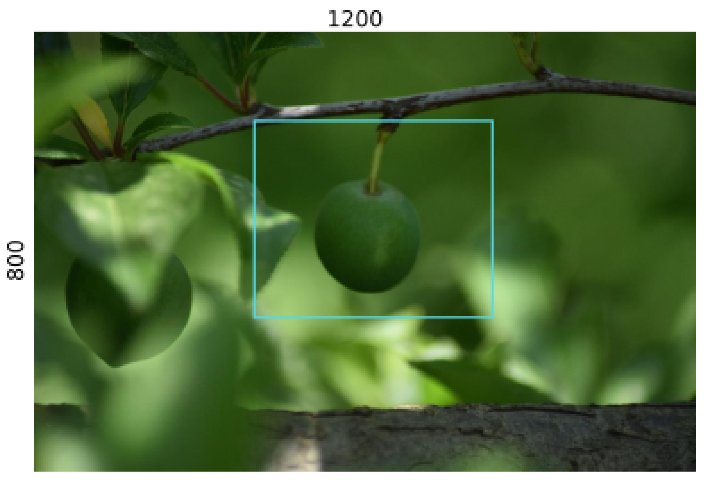
The original images were collected in the plum orchard in real environments without image characteristics concerns. All images are have 1200 pixels in width and 800 pixels in height; however, in the majority of the cases, there is a lot of unnecessary information in the image because the fruit (plum) occupies a small part of the image that is typically centered despite as shown in Figure 5. The Black Diamond variety images were only collected in three different weeks for the 2018 year. Due to logistic restrains, the natural ripening cycle is of 2 to 3 months.

As mentioned before, we will use neuronal networks for the classification process, particularly a CNN called AlexNet that was previously described. This network was designed for classification problems, and its architecture uses RGB images as inputs. The input images sizes are typified as squares of 256 pixels; thus, images with different sizes have to be transformed to the input square size. Usually, resizing or crop transformations or both are used to accomplish the desired size. During our study, we tested two different techniques for image size transformation, which resulted in two different datasets with different preprocessing techniques. We constructed two different datasets using different preprocessing techniques, each one with advantages and disadvantages. 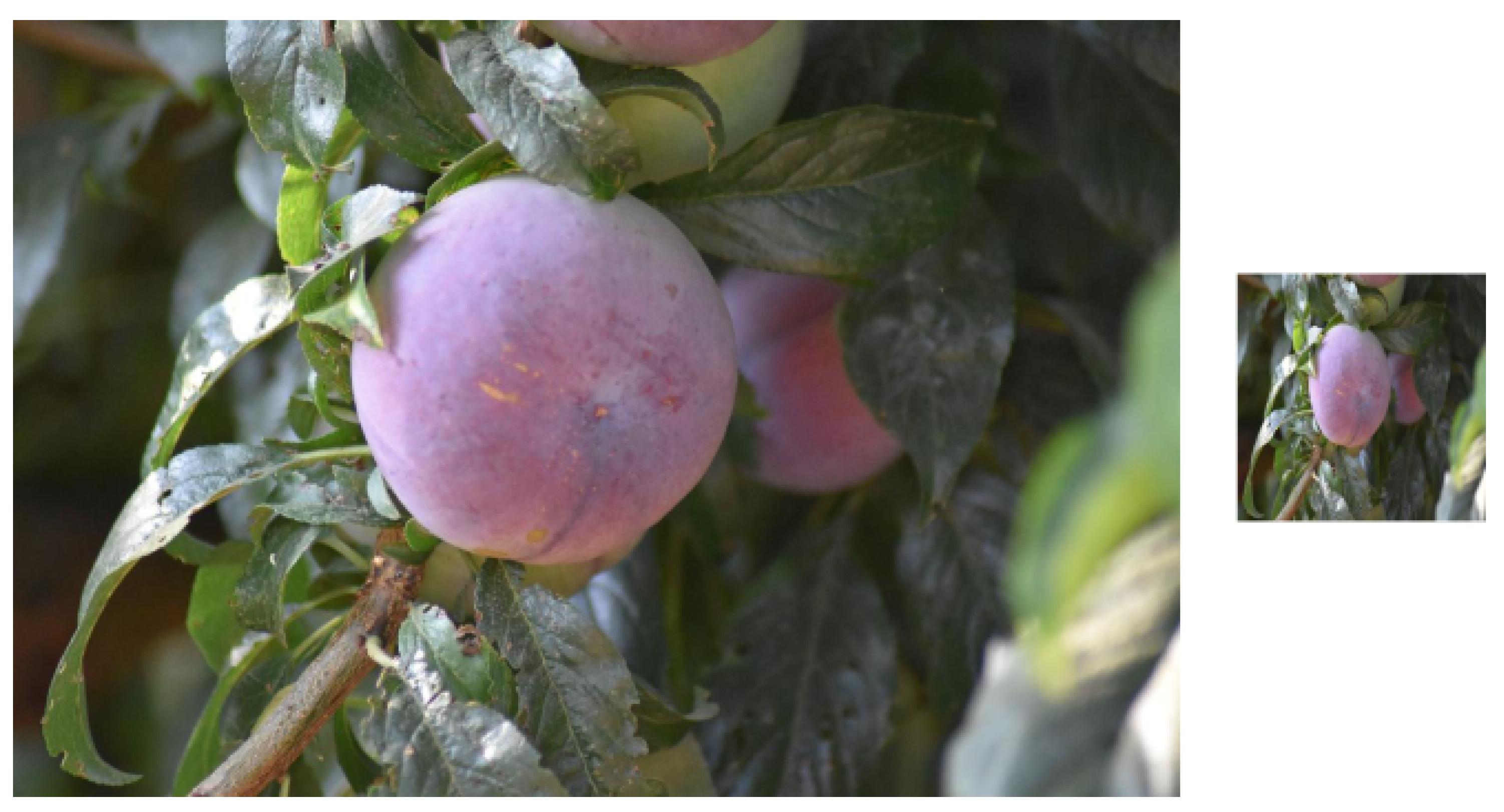As depicted in Figure 6, the first method consists of making a direct resize of the original images, from 1200 × 800 to 256 × 256. This kind of preprocessing does not maintain the image’s proportions and causes distortion; however, it retains all image information, including the borders. The obtained dataset will be called direct resized (DR). 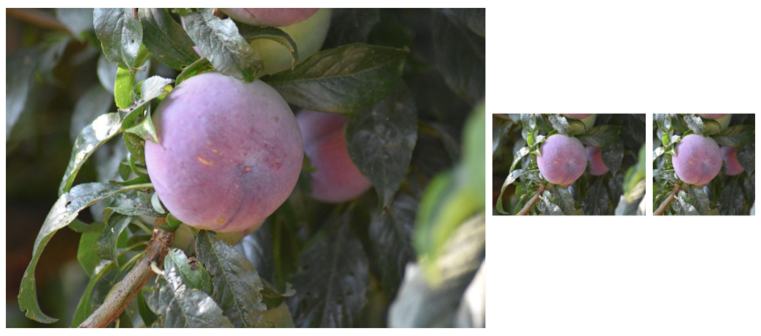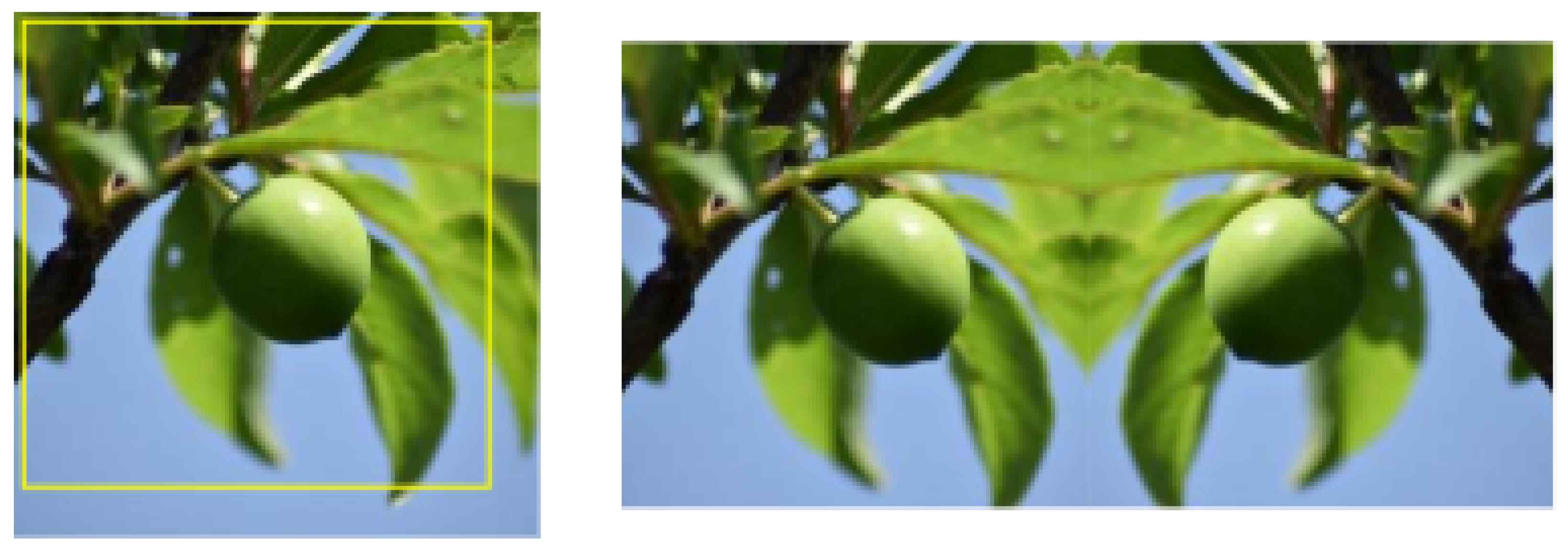The second method used for preprocessing is illustrated in Figure 7, and this technique begins with a proportional resize of the image where the image proportions are kept. An image resize is computed by transforming the smaller dimension from 800 pixels to 256 pixels; the larger dimension is also resized but in the same scale, $\frac{256}{800}$, obtaining a dimension of 384 pixels. Thus, the intermediate image is $384\times 256$. Then, the image is cropped in its horizontal dimension, $\frac{(384-256)}{2}$; this means a crop of 64 pixels at each image side. This method keeps the image proportions without any distortion; however, some parts of the image are lost, particularly the border sides. As observed in Figure 5, the portion of the image that contains the fruit is usually relatively centered, and the crop almost does not affect the image information. This last method results in another dataset used in the experiments, and we will refer to it as resized and cropped (RC). Thus, for the purpose of plum variety classification, we developed two different datasets from the original database of images: DR and RC.

Therefore, the main goal of training a CNN is not to learn the data used during training but rather to be able to correctly classify unseen samples. A successful training session with the entire set would guarantee the required accuracy of the samples of the dataset, but this does not imply being able to obtain a similar or even acceptable level of accuracy on new data. Considering this, we can divide the dataset into two subsets: the training set and the validation set [34]. However, the original dataset could also be partitioned in order to produce a third subset: the testing set.

The training set is used to fit the model. The network weights will be updated from it. The training set must be representative so that the model can learn the most important features to distinguish all classes. The accuracy on the training set tells us if the network configuration used is able to learn the data. Thus, if the model does not perform well on the training data, this means that the network architecture must be reviewed and improved.

A validation dataset is a dataset of examples used to tune the hyperparameters (i.e., the architecture) of a classifier. It is sometimes also called the development set or the “dev set.” An example of a hyperparameter for artificial neural networks includes the number of hidden units in each layer. The testing set (as mentioned above) should follow the same probability distribution as the training dataset.

In order to avoid overfitting, when any classification parameter needs to be adjusted, it is necessary to have a validation dataset in addition to training and test datasets. For example, if the most suitable classifier for the problem is sought, the training dataset is used to train candidate algorithms, and the validation dataset is used to compare their performances and decide which one to take; finally, the test dataset is used to obtain performance characteristics such as accuracy, sensitivity, specificity, F-measure and so on. The validation dataset functions as a hybrid: it comprises training data used for testing but neither as part of the low-level training nor as part of the final testing.

An application of this process is in early stopping, where the candidate models are successive iterations of the same network, and training stops when the error on the validation set grows and chooses the previous model (the one with minimum error). A test dataset is a dataset that is independent of the training dataset but that follows the same probability distribution as the training dataset. If a model fit to the training dataset also fits the test dataset well, minimal overfitting has taken place. A better fitting of the training dataset as opposed to the test dataset usually points to overfitting.

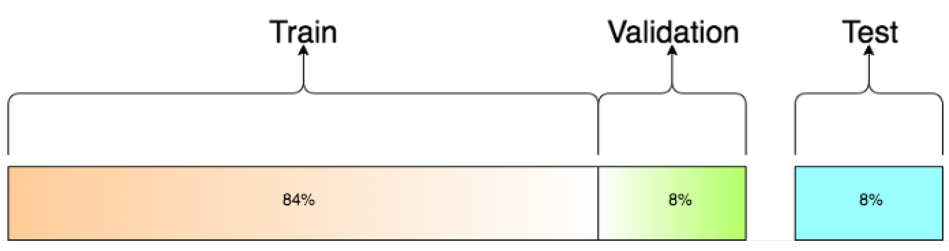
A test set is, therefore, a set of examples used only to assess the performance of a fully specified classifier such as many other aspects in DL; the train–test–validation split ratio is also quite specific to this use case, and it becomes easier to make judgement as we train and build more and more models. In our cases, we have three classes with unbalanced datasets, and all of them have the same importance in the classification problem and training; thus, it is important to keep the proportion or the probability distribution of the three classes in all subsets, training validation and test. In our case, we decided to use 84%, 8% and 8%, respectively (see Figure 8).

4.2. Preprocessing

Some preprocessing operations are required to apply to the input images inputs, usually related with size or with the range of value representations. Typically, AlexNet receives images represented on an RGB colour space; this means that the images are three-dimensional arrays or a set of three matrices usually named channel one matrix for each Red, Green and Blue channel. The typical AlexNet implementation uses square images $227\times 227$ pixels as patches of the original images. However, we may consider the image size 256 × 256, since almost every implementation cropped the original image for data augmentation purposes. We used square RGB images $256\times 256\times 3$ with pixel values in the range $\left[0;255\right]$. 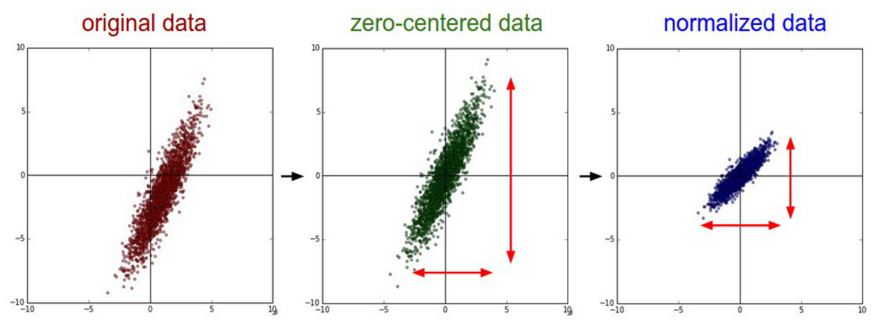To provide a more balanced set, it is common to zero center the pixel values. This can be performed simply by shifting all pixel values from the interval $[0;255]$ to $[-127.5;127.5]$. A more sophisticated approach computes the average image or the mean pixel of the training set and subtracts one of them from all input images. The mean image is represented by an image with a crop size, and the mean pixel is represented by a vector with three elements, $\left[M_R{M}_G{M}_B\right]$, where each element represents the mean value for the image channel. In this manner, we obtain a pixel value representation that is zero centered. These input intervals may cause the weights from the first layers, which are those that are more directly affected by the magnitude of the inputs, to receive large updates, causing an erratic learning procedure. It is common to use a normalization process to transform the values in the range $[-127.5;127.5]$ to a normalized range $[-0.5,0.5]$, and we used a multiplier $(1/255)$ for scaling. We can also use normalization by standard deviation, which will provide a dataset dependent interval, but on average the range remains similar. Figure 9 illustrates the pipeline process with 2D data for better visualization from the original data to the re-centered data and the value range normalization.

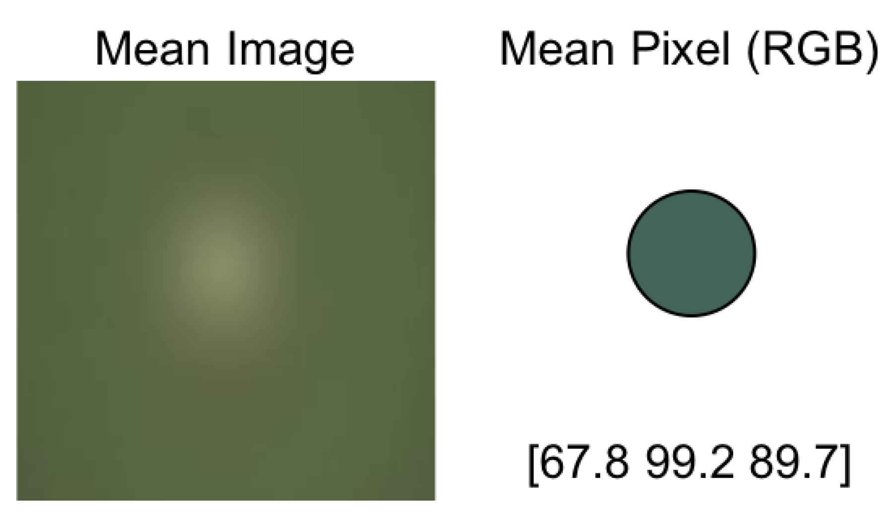
For image pixel values preprocessing, we applied two subtraction techniques during our experiments stage, the mean image subtraction (MI) and the mean pixel subtraction (MP), and we created Figure 10. We demonstrate the mean image representation obtained for a training dataset, and we also show mean pixel values computed for the same training dataset.

4.3. Data Augmentation

Showing different variations of the same image to a neural network helps prevent over-fitting as it is forced to not memorize the images. Often, it is possible to generate additional data from existing data in an easy manner [35]. Among the many possibilities, we used two combined techniques: image translations and image reflections. The image translations consist of extracting random square patches from the $256\times 256$ image, usually $227\times 227$. Each patch is also horizontally reflected (mirroring), Figure 11. During our experiments, different square crop dimensions were used and tested. These two operations, translation and reflection, increase the size of our training set, and we used the resulting patches as inputs of the network (input images are $227\times 227\times 3$-dimensional because we assumed the square crop of 227 pixels).

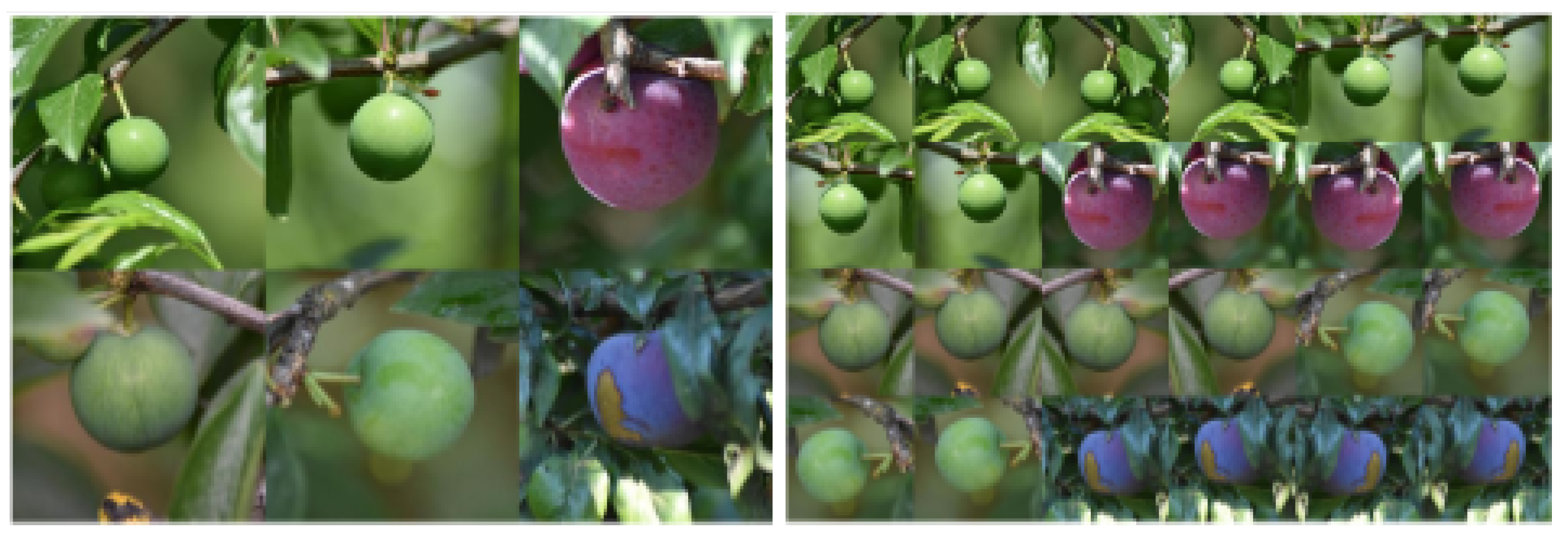
During the test stage, the prediction was performed by using several cropped smaller images extracted from the original and their horizontal reflection: five extracted images sized $224\times 224$, four for each image corner and a centered one. These five images and the reflections are classified, and the final result is made by using the average of the result of the final softmax layer of the network. In Figure 12, we are able to observe six original images and the resulting augmented dataset by using image random crops and horizontal mirroring.

During the plum variety problem study, we had more then a 1500 images per class in the worst scenario, and some classes had more than 4000 images. However, for the ripening study, the number of classes is larger for each variety, and the total number of images is smaller once we had to split the plum dataset into three independent datasets. For the Angeleno ripening classification, we have a total of 4773 images for 10 ripening classes that correspond to a mean of 477 images per class. Aware of this potential problem, we applied an additional data augmentation process based on image rotations that have a larger base for a better training process. Each original image suffers a positive and negative rotation with 30${}^{\circ }$ before the resize and crop processes; therefore, we multiply by three the number of images for each class, achieving a larger image dataset that is important for the network training stage in DL. The process is illustrated in Figure 13.

4.4. Networks Architecture

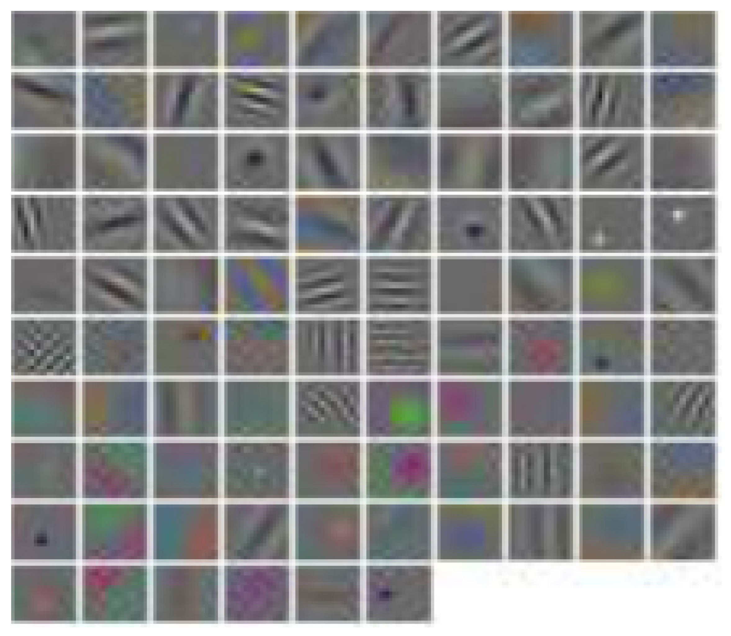
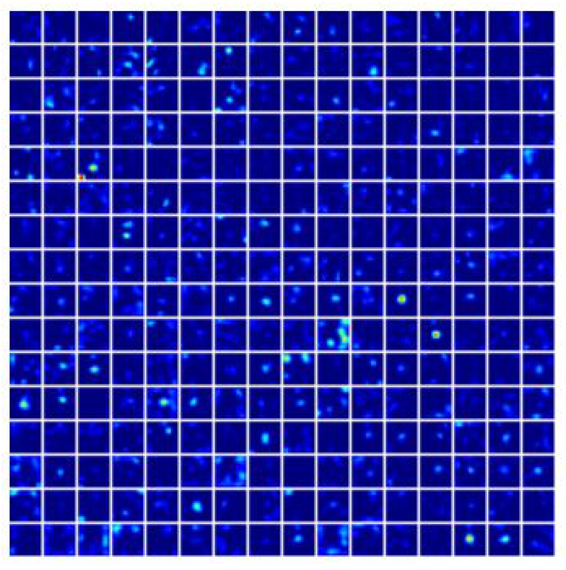
Our two classification problems use a CNN architecture based on AlexNet [3] with slight changes. Moreover, in the AlexNet layers, we are able to observe the kernels as well as the ReLUs and max pooling processes. The CNN is built by using eight layers and their corresponding weights: the first five layers are denominated convolutional layers (conv), and the following three layers are fully connected layers (FC). The last layer output is computed using a n-way softmax function. This softmax layer computes a probability distributions over the n classes (labels) used. For the variety classification problem, the number of classes is three. Although for the ripening problem, the number of classes proceeds from 3 to 11. To describe the network architecture and related processes, take as example the variety problem with three classes. For the remaining networks of the ripening problem, it is sufficient to change the number of classes according to each case. The first layer is a convolutional layer, and it computes several convolution between the 227 × 227 × 3 input image and 96 filters or kernels sized 11 × 11 × 3; the convolutional process uses a stride of four pixels. An example of those training kernels obtained for the plum variety classification problem is shown in Figure 14.

The second layer, also a convolutinal layer, receives the output of the previous layer after a process of maximum overlap pooling and uses 256 kernels with sizes of 5 × 5 × 48 with respect to the convolutional process. The third layer uses the output of the second layer after the maximum overlap pooling process and convolves it with 384 kernels of size 3 × 3 × 256. The fourth convolutional layer uses 384 kernels with 3 × 3 × 192, and the last convolutional layer has 256 kernels of size 3 × 3 × 192. When the max pooling process is used, there is also a normalize process. Each of the following fully connected layers contains 4096 neurons, and the last layer performs a three-way softmax according the example in Equation (1).

$$y=\left[\begin{array}{c}2.0\\ 1.0\\ 0.1\end{array}\right]\to S\left(y_i\right)=\frac{e^{y_i}}{{\sum }_i^{}{e}^{{}^{{}^{y_i}}}}\to p=\left[\begin{array}{c}0.7\\ 0.2\\ 0.1\end{array}\right]$$

(1)

The Softmax transforms the y values into p probabilistic distribution values over three class labels. Our network uses the average across training cases of the log-probability of the correct label under the prediction distribution to compute loss [3]; it is equivalent to the cross-entropy (Equation (2)).

$$L=-\sum _{i=1}^M\sum _{c=1}^3\left(y_{c,i}·log\left({\widehat{y}}_{c,i}\right)\right)$$

(2)

The goal is to minimize the loss function (L), where c represents the image class, and i is the image number in the training set with M images. The $\widehat{y}$ values are the model’s prediction (i.e., the output of the softmax for a class), and y values correspond to the class labels: one-hot encoded, zeros or ones. During the training process, we used back propagation to compute the gradient, and stochastic gradient descendent (SGD) [36] is used as optimization method, namely first order optimizer; this means that it is based on analysis of the gradient of the objective. Consequently, in terms of neural networks, SGD and backpop are often applied together to make efficient updates. The updating rule for weights $\left(w\right)$ during the training process is based on SGD, modeled by Equations (3) and (4).

$$v_{i+1}:=0.9·v_i-0.0005·ϵ·w_i-ϵ·{〈\frac{\partial L}{\partial w}{\mid }_{w_i}〉}_{D_i}$$

(3)

$$w_{i+1}:=w_i+v_{i+1}$$

(4)

i represents the iteration number, v is the momentum variable, $ϵ$ is the learning rate and ${〈\frac{\partial L}{\partial w}{\mid }_{w_i}〉}_{D_i}$ is the average of the $i$th batch $D_i$ of the derivative of the objective with respect to w, evaluated at $w_i$ [3].

4.5. Transfer Learning

Transfer learning generally refers to a process where a model previously trained on one problem is used in some way on a second related problem.

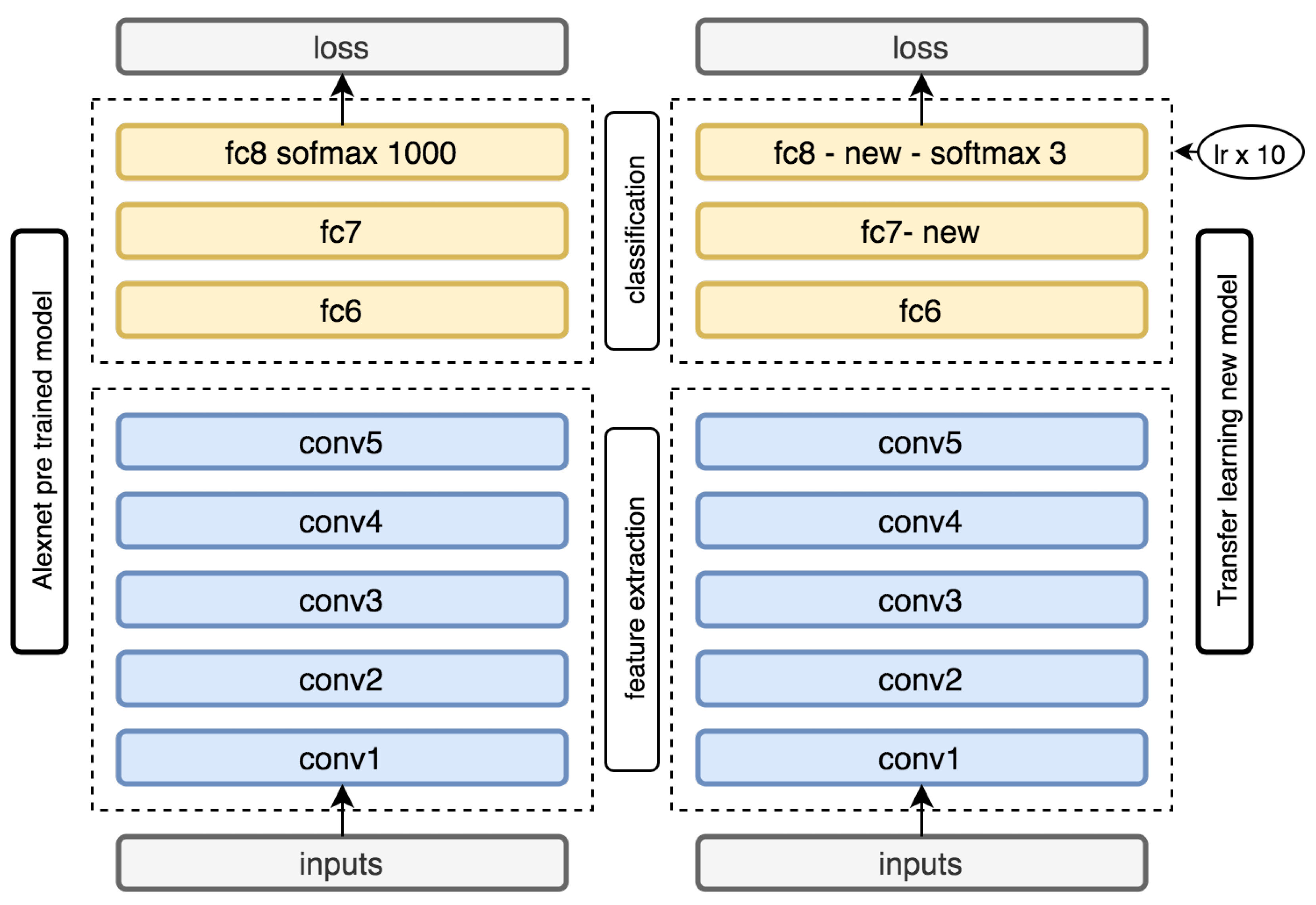
In DL, transfer learning is a technique whereby a neural network model is first trained on a problem similar to the problem that is being solved. One or more layers from the trained model are then used in a new model trained on the problem of interest. Transfer learning has the benefit of decreasing the training time for a neural network model and can result in lower generalization error. The weights in re-used layers may be used as the starting point for the training process and adapted in response to the new problem. This usage treats transfer learning as a type of weight initialization scheme. DL systems and models are layered architectures that learn different features at different layers (hierarchical representations of layered features). These layers are then finally connected to a last layer or a group of layers, usually fully connected to obtain the final output. This layered architecture allows us to utilize a pre-trained network without its final layer or layers as a fixed feature extractor for other tasks (Figure 15).

Our type of problem constitutes a typical image classification problem; thus, we used, as a basis for the transfer learning process, the AlexNet architecture and a pre-trained model. Considering the layer architecture of AlexNet, we used a natural subdivision into two groups of layers; the first five convolutional layers compose feature extraction, and the last two fully connected layers are responsible for using those features to produce a valid classification of the image. Thus, we built our transfer learning model by using part of the AlexNet pre-trained model, and we used the five initial layers with weights and biases previously trained for the ILSVRC2012 image classification competition. We substitute the last two fully connected layers by two new similar layers (fc7 and fc8), as shown in Figure 15. The last layer uses softmax to compute classification and loss during training. To train the new model, we used the pre-trained model values for the bottom layers (feature extractor), and we randomly initialized the newly added layers. During the training stage, we used different learning rate multipliers for different layers. We used a larger learning rate multiplier ($\times 10$) in the new fully connected layers. In this manner, we ensure that the classification layers suffer larger and faster changes during the training process, and the convolutional layers from the feature extractor have smaller and finer changes. This process is denominated fine tuning.

5. Experiments and Results

To conduct the experiments, we take in account the two problems studied, variety and ripening, in addition to the combined two-stage problem where we predict the ripening in weeks of a plum using an image without previous know of its variety. All the experiments were performed in a server by using a graphics card “NVIDIA GTX 1080 Ti” for the training stage and test stage. Therefore, this section will be divided into three different sub sections: Section 5.1 analyzes the variety classification problem from scratch by using deep transfer learning. Then, we present the experiments for the ripening problem in Section 5.2. Finally, we present the results for the combined two-stage problem in Section 5.3. The results obtained during the experiments for the first problem were used to configure parameters for the next problem, and the same approach was used for the second and third (combined) problems.

5.1. Variety

Our first problem is plum variety image classification. Using DL, it is important to notice that the images are collected in the field and, thus, in the fruit’s natural environment, with trees and leaves. Additionally, the fruit images are tokens of different weeks and years; thus, they are in different ripening stages (from the fruit set with small size to the time of harvest). For the plum variety study, we will use two different approaches, both of them based on CNN AlexNet. The first technique consists of training the network from scratch with different hyper parameters. The second methodology is based on transfer learning using a pre-trained model.

5.1.1. Original CNN

We used the CNN AlexNet architecture to make our first experiments by training the network from scratch. This set of experiment was our first approach to tackle this problem, which is a typical image classification one. The network architecture slightly changed, and we substituted the last fully connected layer by one, with three outputs computing softmax. Each output corresponds to a class of our three classes problem: Angeleno, Red Beaut and Black Diamond.

To perform the training process, we used the 2018 image database (Table 1). From this group of images, by using different image preprocessing techniques, we created two distinct image datasets: DR based on resizing and RC created by using a resize and crop process, both described in Section 4.1. Both datasets have a training set, a validation set and a test set size of 84%, 8% and 8%, respectively.

We tested another two parameters related with image transformations in our first set of experiments: the crop size for data augmentation and image normalization. Both techniques are described in Section 4 and are data transformation processes for better representation or augmentation data. We tested crop sizes of 227 and 200 pixels, and we tested also the normalization process using the mean image (MI) and mean pixel (MP). The other parameters were kept constant at a certain learning rate (0.01), and the number of epochs for training was 300. All parameter value combinations were tested, and the results are presented using mean accuracy in percentage and standard deviation (

Table 2. Experiment results for the plum classification problem using DL from scratch with different parameters values, 2 different datasets (RC and DR), 2 normalization methods (mean image and mean pixel), w different crop sizes for data augmentation (227 and 200), learning rate of 0.01 and 300 epochs during training. Mean accuracy results and standard deviation were obtained from 10 repetitions of each experiment.

Network/Method	Data Set	Crop Size	Normalization	Accurracy (%)	S.D.
AlexNet From Scratch	RC	227	MP	88.32	0.58
	RC	200	MP	87.73	0.35
	RC	227	MI	87.54	1.36
	RC	200	MI	87.98	0.38
	DR	227	MP	87.34	0.58
	DR	200	MP	88.21	0.74
	DR	227	MI	87.66	0.21
	DR	200	MI	87.99	0.16

).

All the experiments have results in the range $[87\%,89\%]$. These are mean values of 10 repetitions with standard deviation of less than $1.5\%$, which indicates that the random component inherent to the initialization of the network parameters does not affect accuracy results in a significant manner. The accuracy results are those obtained by using the validation dataset disjoint from the training set; however, some preliminary conclusions can be made. The experiments that use mean pixel (MP) have slightly better performances over those who use mean image (MI). The RC dataset works better with 227 crops and the DR dataset has better results with 200 crop size. This is due to the image process transformations used to build each dataset; the RC has already a crop in width. We also conclude that our network with best accuracy uses the RC dataset, with a crop size of 227 and normalization process based on MP with LR of 0.01. We computed the confusion matrix for our three classes problem by using our best network parameters. Two confusion matrices, usual and normalized, were made by using the test subset (8%) of the dataset (unused and disjoint). The detailed results can be observed in Figure 16.

It is possible to observe that Angeleno is the most accurate class, and Red Beaut is the worst in terms of accuracy with a 15% gap; it is also related with the number of images of each class used on the training stage and proportional to those used on testing. The confusion matrix allows us to calculate other evaluation metrics; we computed precision, recall and F-measure for each class using the data presented in Figure 16. The Angeleno class was 0.932, 0.927 and 0.929, respectively. The Red Beaut class was 0.709, 0.678 and 0.693. The Black Diamond class was 0.852, 0.870 and 0.861. The system’s overall F-measure was 0.869. For further analysis and experiments, we will consider the mean pixel as a normalization process as well as the use of the RC dataset.

5.1.2. Transfer Learning

The next set of experiments is based on the transfer learning technique. We used a pre-trained model of AlexNet that includes part of the architecture and part of the weights, and we introduced some changes. We trained the entire network with some parameterizations (Section 4.5). Based on the scheme presented in Figure 15, we introduced some changes in the top layers, particularly to the top two layers.

For transfer learning, we substituted the last fully connect layer (fc8) for a new one with three outputs (one for each class). We also substituted the penultimate layer (fc7) for a new identical layer. In this manner, the first six layers are imported from the pre-trained model including weights and biases, and the last two layers are replaced; thus, they have no trained values. We could replace all the classification layers from the model (last three) (see Figure 15) by using the feature extractor from the pre-trained model (first five convolutional layers); however, preliminary tests showed that the last two layers or even only the last one possess better results for this kind of classification problem.

Thus, we used two different network models for the transfer learning process: The first one only replaced the last fully connected layer, and the second replaced the last two fully connected layers. In both cases, they use the feature extractor output, illustrated in Figure 17, and are computed by using an example image. These outputs are passed by a pooling processor for data dimension reduction and will be the inputs for the classification part composed of the fully connected layers. We also introduced a learning rate multiplier for the new layers (10 times).

The new set of experiments for the transfer learning method take in account the results of the previous set of experiments presented in Table 2. There, we saw that the MP method for normalization stands out, as well as the combination of RC with a crop size of 227 and DR with crop size of 200 with a slight advantage to RC. We used three different image databases, one from 2018 and the other from 2019; finally, a larger one that combine images collected during those 2 years was used.

In

Table 3. Experiment results for the plum classification problem using transfer learning with 3 different image data bases: results for mean accuracy and standard deviation from 10 repetitions for each experiment.

Network/Method	Data Set	Year	Crop Size	Normalization	N. Layers	Lr(X)	Acc. (%)	S.D.
AlxNet TL	RC	2018	227	MP	1	10	93.66	0.11
	DR	2018	200	MP	1	10	93.26	0.54
	RC	2018	227	MP	2	10	93.85	0.13
	RC	2019	227	MP	2	10	88.93	0.04
	RC	2018/19	227	MP	2	10	91.66	0.14

, the results obtained for the validation datasets after training the networks with the expressed parameters values are presented. Some parameters stay constant for all sets of experiments: mean pixel for normalization, learning rate multiplier ($10\times$) for new layers, 300 epochs for each experiment and 10 repetitions. We trained the 2018 database image using the two different technique described earlier, the resize and crop(RC) and direct resize (DR), and we used the parameters values that achieved the best results in the previous experiments (Table 2). The dataset RC with a crop size of 227 and dataset DR with a crop size of 200 both used the mean pixel (MP). The RC dataset obtained more than $0.4\%$ in accuracy compared with DL, achieving $93.66\%$. We also tested the influence of one or two completely new layers in the transfer learning process. We conclude that the use of two new layers is slightly better in terms of accuracy, which is $93.86\%$ compared with $93.66\%$. Therefore, we took in account the obtained results and extended the experiments to the new image databases, which is from year 2019 and the combination of 2018 and 2019. We kept the best parameters values tested before: dataset process RC, crop size 227, normalization using MP and two new layers. We obtained the following results: for year 2019, accuracy was $88.93\%$, and for the combined years 2018 and 2019, accuracy was $91.66\%$.

The results shown in Table 3 are expressed in accuracy percentage, obtained from the validation sets. We used the network configuration with the best performance for the 2018 database, and we kept the network parameters for the 2019 database and for the 2018 and 2019 joined database in order to perform more detailed tests. We tested the networks using the test sets for each image database, and we calculated the confusion matrices for the three cases Figure 18. For the 2018 database, we obtained an overall accuracy of $93.4\%$, and the Angeleno class is the most accurate, reaching $96.5\%$, in contrast to Red Beaut, which had $86.0\%$. Finally, the Black Diamond variety had $92.3\%$. The gap of almost was $10\%$, which is derived from the number of images of each class that made up the dataset. Classes with fewer images had worst accuracy results: In this case, the Black Diamond image dataset was smaller than one-third of the other two classes (Table 1). This fact results in an increase in the probability of overfitting, and this may occur at an earlier stage of the training process. When overfitting occurs, the accuracy results for training are not extended for the unused test-set. The 2019 database is even smaller than the 2018 one, and the accuracy is $88.4\%$; in this case, the class with less images and less accuracy is Angeleno.

Finally, we built a general dataset combining the images from 2018 and 2019 after training. The result obtained for the classification process using the test dataset was $90.1\%$. Here, we can observe that the Red Beaut class is the most accurate, $93.3\%$; it is also the class with the highest number of images, which is almost 7000. For all three image databases used, the accuracy results are higher then $90\%$, which is a very secure result for this kind of classification problem, using images captured in real fruit environment. Using the data depicted in the confusion matrices (Figure 18), we computed precision, recall and F-measure for the 2018/2019 dataset for each class, and we obtained the following results: Angeleno (0.915, 0.905 and 0.910), Black Diamond (0.920, 0.838 and 0.877) and Red Beaut (0.847, 0.933 and 0.889). The methodology based on deep transfer learning presents better results than the methodology based on training the network from scratch. As explained earlier, the fruit images have a high variation; however, the network performs well, as observed in Figure 19 (where nine images per class correctly classified by the system are depicted).

5.2. Ripening Classification Process

The classification process is based on convolutional neural networks with an architecture based on AlexNet, using transfer DL. The images database and subsets are the same as the previous study (Table 1); however, we will only use the subset of 2018 due to the labeling process in field. For this problem, the 2018 image database is organized in a different manner. The image database is divided in ripening weeks for each variety, resulting in 10, 3 and 11 classes for Angeleno, Black Diamond and Red Beaut, respectively. In this manner, we will have there networks with more classes and with fewer images, which a challenge for us. To build the datasets for each of the three networks, we use the resize and crop process (RC), as well as the split in training validation and test subsets, described in Section 4.1.

With respect to the ripening study of the three plum varieties, we considered two sets of experiments: one using the usual data augmentation process also applied to the precious experiments, based on mirroring and crops, and the other in addition to the usual uses, with an additional data augmentation process based on positive and negative rotation described in Section 4.3. The experiments are characterized by the use of transfer learning with two new final layers. The learning rate multiplier for this new layer is $10\times$. Each variety of experiments uses images from the 2018 image database. Each image database is split into labeled folders, and each folder is for each ripening week. The datasets were built by using RC with 512 square crop and data augmentation crop size of 227. Each dataset was also split in training validation and test sets. Images are normalized with MP, the training stage includes 300 epochs, and it is performed 10 times for statistical purposes. Mean accuracy and standard deviation are calculated.

Table 4. Plum ripeness analysis experiments using the default data augmentation process and using an additional data augmentation process with 2 image rotations. Datasets are based on RC process; images are from the 2018 database; ripening weeks and variety; and results of mean accuracy and standard deviation are in percentages.

Aditional Data Augmentation	Data Set	Yeqr	Weeks	Variety	Acc. (%)	S.D.
None	RC	2018	10	Angeleno	72.80	0.38
	RC	2018	3	Black Diamond	75.70	0.58
	RC	2018	11	Red Beaut	73.50	0.74
Rotation 2x	RC	2018	10	Angeleno	94.80	0.69
	RC	2018	3	Black Diamond	98.00	0.42
	RC	2018	11	Red Beaut	94.70	0.41

shows the main parameters and the obtained results. The experiments use the training sets to evolve the networks, and the final results are calculated over the disjoint validation sets.

Figure 20 shows the graph of the training process of one of the experiments using 500 epochs, particularly for ripening of Angeleno with 10 weeks ripening cycle. Table 4 shows all sets of experiments conducted as well as the results in mean accuracy percentage. We are able to infer that the additional data augmentation process increases the accuracy results at over $20\%$. The accuracy values for the set of experiments without additional data augmentation are in the range of $[72\%;76\%]$, in contrast with the much higher values obtained using the rotation with additional data augmentation in the range of $[94\%;98\%]$. The variety Black Diamond with only three classes corresponding to 3 weeks of ripening is the most accurate, reaching $98\%$. In addition to the large number of classes for the other two plum varieties, 10 and 11, the results are very precise: $94.8\%$ for Angeleno and $94.7\%$ for Red Beaut. We also note the importance of the ratio number of images per class for an effective training of the CNN, even when using transfer learning. The overall mean value for accuracy of the ripening problem in knowing the variety is $95.5\%$, which a very strong value considering the number of classes, the image acquisition process in the real environment and the very unperceptive changes in two consecutive weeks.

As in the previous experiments, we also calculated the confusion matrices for each variety for the ripening problem (Figure 21, Figure 22 and Figure 23). The Angeleno variety has a ripening cycle of 10 weeks; thus, we consider 10 different classes for the ripening problem. The classes located in the extremities of the cycle have better results: first 2 weeks, zero and one, and last 2 weeks, 8 and 9 Figure 21. These are the classes where there are more fruit image variabilities. The false negatives of a certain class are false positives of the others, and they are almost located in adjacent classes, typically one week earlier and one week later. The Black Diamond variety has 3 weeks worth of documented ripening cycles (the Black Diamond ripening cycle is 8 weeks long; however, due to logistical problems in 2018, we only documented 3 weeks); thus, the accuracy results are more precise than the other varieties, and all ripening weeks have accuracy results higher than $90\%$ Figure 22. The Red Beaut variety has a ripening cycle that is 11 weeks long, and it is the largest analyzed; however, the accuracy results stay high. Once again, the first 2 weeks have stronger accuracy results; then, the results decrease during the intermediate weeks until they rise again in the last ripening week Figure 23.

5.3. Variety and Ripening

In the previous two sections (Section 5.1 and Section 5.2), we described our approach for two distinct problems: plum variety and plum ripening, respectively. Both problems were tackled as independent problems. According to Figure 2, the problem can be divided into two problems or observed as a combined problem of two stages. Thus, we may consider the variety and ripening as a chained problem with two stages, where the ripening stage depends on the variety stage. The combined problem can also be observed as a estimation problem of ripening of a plum image with unknown variety. We used the combined system with two stages of CNNs to estimate the ripening week of an image without previous knowledge of the variety. We used the 2018 sub-database and the RC method for dataset construction, and the accuracy results were calculated over the unused test set.

Table 5. Plum variety and ripening study accuracy results in percentage: ripening results by variety, by ripening week and overall.

Data Set	Year	Variety	Week	Acc (%)
RC	2018	Angeleno	0	94.80
RC	2018	Angeleno	1	94.80
RC	2018	Angeleno	2	92.90
RC	2018	Angeleno	3	88.16
RC	2018	Angeleno	4	85.32
RC	2018	Angeleno	5	80.58
RC	2018	Angeleno	6	76.79
RC	2018	Angeleno	7	86.27
RC	2018	Angeleno	8	90.06
RC	2018	Angeleno	9	92.90
RC	2018	Angeleno	All	91.48
RC	2018	Black Diamond	0	87.00
RC	2018	Black Diamond	1	80.04
RC	2018	Black Diamond	2	79.17
RC	2018	Black Diamond	All	85.30
RC	2018	Red Beaut	0	88.61
RC	2018	Red Beaut	1	86.76
RC	2018	Red Beaut	2	86.76
RC	2018	Red Beaut	3	84.92
RC	2018	Red Beaut	4	87.69
RC	2018	Red Beaut	5	88.61
RC	2018	Red Beaut	6	77.53
RC	2018	Red Beaut	7	85.84
RC	2018	Red Beaut	9	80.30
RC	2018	Red Beaut	9	73.84
RC	2018	Red Beaut	10	90.45
RC	2018	Red Beaut	All	87.5
RC	2018	All	All	89.4

shows the detailed accuracy results for the overall two-stages system. The results were divided into three variety classes. Each class contains the partial results for each ripening week, and the overall for all weeks are shown in bold. The last result is the overall result calculated for all variety classes, and it reaches $89.4\%$. Therefore, our two-stages classification system is able to estimate the ripening week of a plum using an image acquired in a real environment. It performs the classification task with an overall accuracy of $89.4\%$. The most accurate variety class on estimating the ripening week is Angeleno with $91,48\%$, followed by Red Beaut with $87.5\%$ and Black Diamond with $85.3\%$. As expected, the accuracy results for the combined problem is lower than any of the problems studied independently (variety or ripening). As far as we know, there is a lack of research in fruit ripeness analysis using computer vision for images captured in the field and including the variety problem; however, we may compare our results with [18], which performs ripeness analysis on palm oil fruit with some constraints in the image-capture process and presents accuracy results between $80\%$ and $90\%$. If we consider our one problem approach (only the ripeness), the obtained results are higher than $94\%$. Considering the two problem approach, which includes variety classification and ripeness analysis and is a more complex classification problem, the overall results reach $89.4\%$. All the experiments include a high time consumption training stage, between 2 and 3 hours depending on the number of images used; however, classifying a particular image using one of the trained networks is an almost instantaneous process.

6. Conclusions

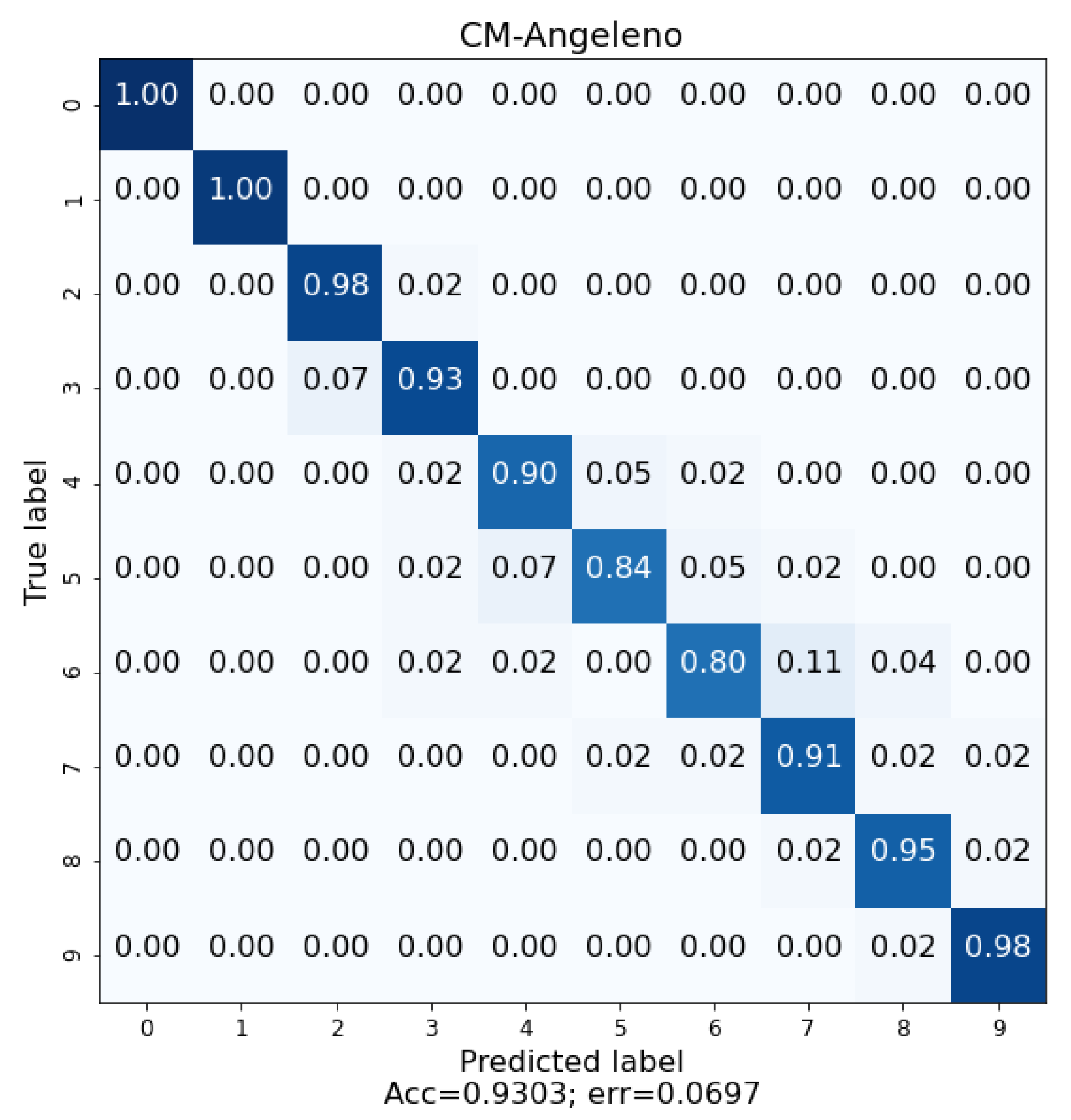
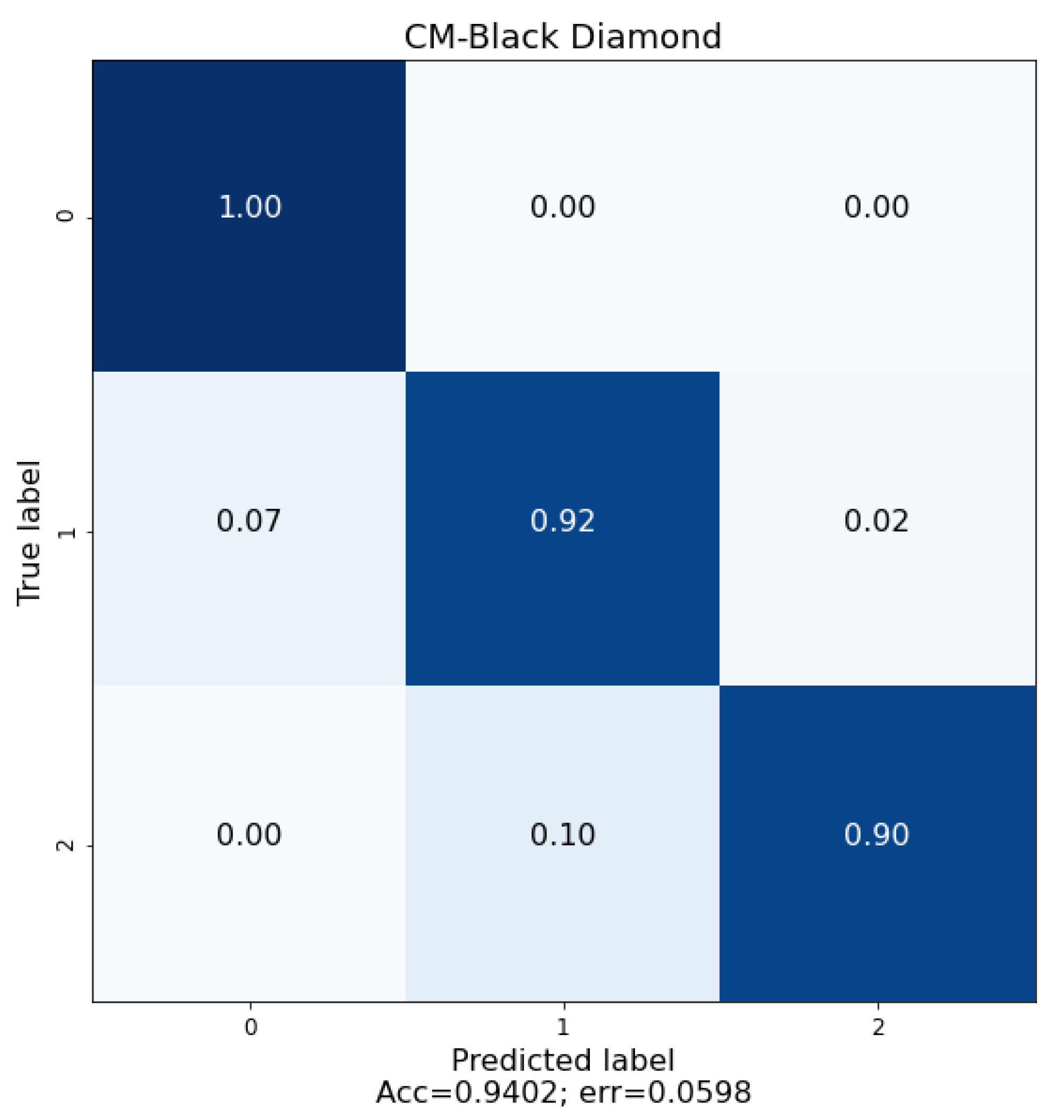
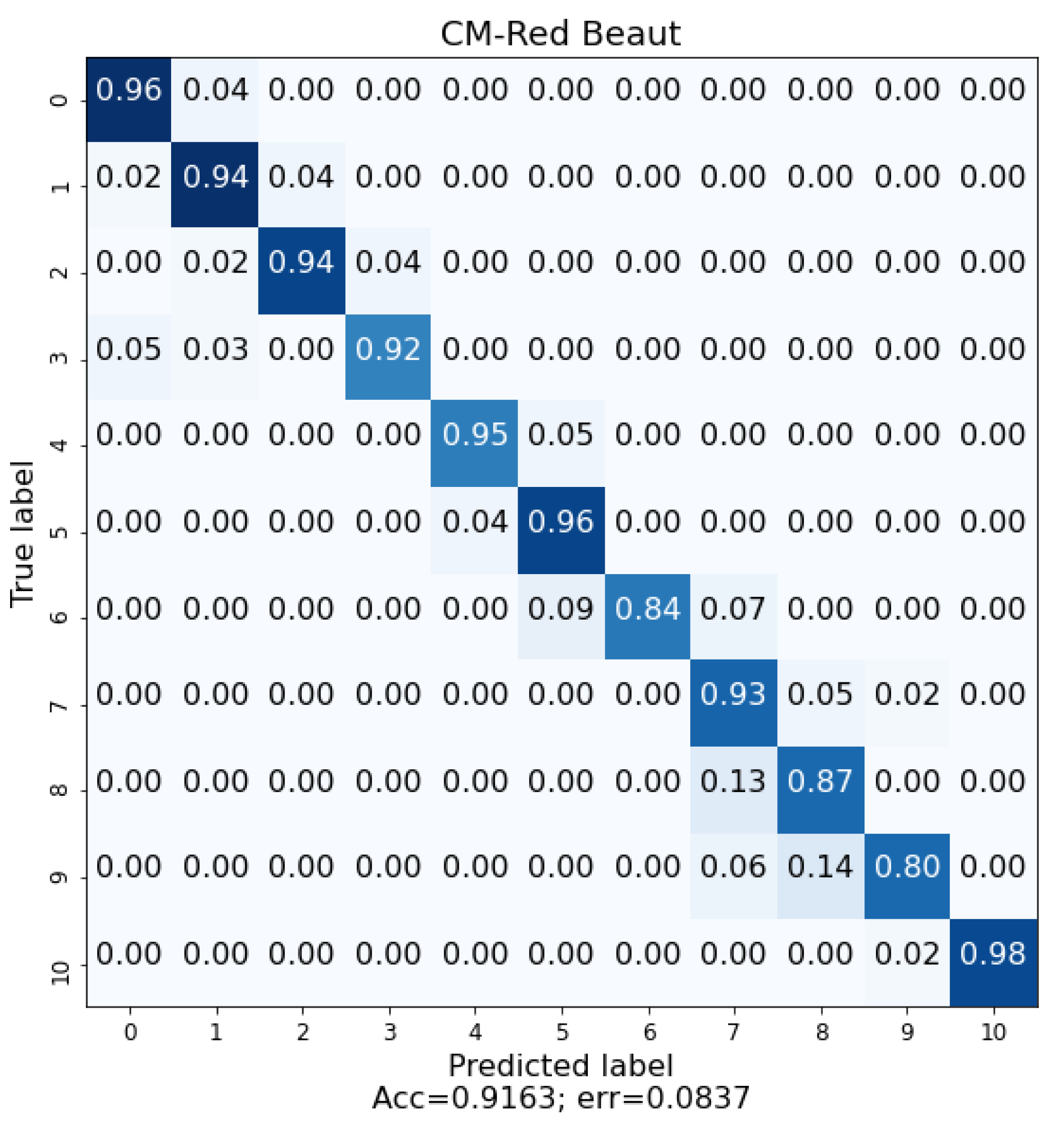
The cultivation of plums in Extremadura is very important, as the main activity of the region is centred on the primary sector. The digitalization in modern agriculture arrived to stay, and it is a fundamental tool nowadays. The crops are tracked by set of modern sensors that provide important information to farmers, allowing them to observe, in real time, the state of their crops. This modernization process results in important cost savings and in higher quality harvests. In this research study, we present and detail a research investigation with a tool based on DL that is able to differentiate three different plum varieties as well as their ripeness state by using images analysis. This system novelty consist of unsupervised and unconstrained conditions with respect to image acquisition. The algorithm was designed to work with uncontrolled photographic acquisition conditions. Therefore, the users can take a photograph with any device, camera, smartphone, etc., in the plum’s real environment, the orchard, regardless of the climatic conditions, light, focus and without centering or zoom restrictions. The system presents an accuracy of 92.83% for three varieties of plum by using images acquired directly in the field, Angeleno, Red Beaut and Black Diamond, with different ripening cycles. The system demonstrates a mean accuracy of 95.5% in the analysis of the ripeness of the plum, with knowledge its variety. This has allowed us to obtain a robust classification system that will allow users to differentiate between these varieties and their ripeness week. In future studies, we should try the same study but by using other more recent network architectures in addition to AlexNet.

The incorporation of artificial intelligence, particularly computer vision-based algorithms, in agriculture will allow farmers and technicians to have decision support systems available to them thanks to the amount of data that can be analyzed in a short period of time. The system presented in this article, once implemented in easy-to-use devices for farmers such as smartphones, will provide them with a tool that will allow them to observe the state of their orchards. The data presented in this paper are very promising for the advancement of Extremadura’s countryside.