Estimation of the Hourly Global Solar Irradiation on the Tilted and Oriented Plane of Photovoltaic Solar Panels Applied to Greenhouse Production

Abstract

Agrometeorological stations have horizontal solar irradiation data available, but the design and simulation of photovoltaic (PV) systems require data about the solar panel (inclined and/or oriented). Greenhouses for agricultural production, outside the large protected production areas, are usually off-grid; thus, the solar irradiation variable on the panel plane is critical for an optimal PV design. Modeling of solar radiation components (beam, diffuse, and ground-reflected) is carried out by calculating the extraterrestrial solar radiation, solar height, angle of incidence, and diffuse solar radiation. In this study, the modeling was done using Simulink-MATLAB blocks to facilitate its application, using the day of the year, the time of day, and the hourly horizontal global solar irradiation as input variables. The rest of the parameters (i.e., inclination, orientation, solar constant, albedo, latitude, and longitude) were fixed in each block. The results obtained using anisotropic models of diffuse solar irradiation of the sky in the region of Castile and León (Spain) showed improvements over the results obtained with isotropic models. This work enables the precise estimation of solar irradiation on a solar panel flexibly, for particular places, and with the best models for each of the components of solar radiation.

1. Introduction

The solar irradiation incident on the surface of a solar panel is the fundamental parameter for the design of photovoltaic systems that are best integrated into greenhouses for agricultural production and for determining the amount of electrical energy that is produced by such a panel, as well as for the simulation of its operation with the required precision. The value of the solar radiation that affects the solar panels is the main variable needed to determine the performance of a photovoltaic (PV) system, together with the ambient temperature, humidity and the speed and direction of the wind (see Pérez-Alonso et al. [1]).

In modern agriculture, greenhouses are intended to increase the productivity, quality, and precocity of crops that are characterized by the intensive use of land and of other means of production and inputs (see Yano and Cossu [2]). Greenhouses, except those located in large, protected production areas, are usually located in rural off-grid areas, and connection to the grid can be very expensive for technical, economic, or environmental reasons; therefore, an autonomous power source is required (see Chaurey and Kandpal [3] and Qoaider and Steinbrecht [4]). Thus, an efficient framework is needed to use solar/diesel systems in off-grid greenhouses (see Cai et al. [5]). On the other hand, the highest electrical consumptions in greenhouses correspond to ventilation, refrigeration, and pumping equipment (water and nutrients). These agricultural structures are usually located in open spaces where they receive large amounts of direct solar radiation. Hence, the largest demand for electricity occurs during periods in which solar irradiation is available in large quantities, thus matching the demand and supply, which makes the use of solar energy viable (see Al-Ibrahim et al. [6]).

To estimate the incident solar irradiation, a pyranometer can be used [7], installed in the same solar panel plane that is to be studied [8], and if such a sensor is not available, its value can be estimated with the measurements of pyranometers installed in nearby meteorological stations, from which such measurements are normally taken on the horizontal surfaces.

The solar irradiation received by a solar panel inclined at a certain angle with respect to the horizontal surface and oriented with a deviation towards the east or west with respect to the equator, with respect to the solar irradiation that reaches the horizontal surface, which is usually measured and recorded in meteorological stations, depends on various variables and parameters. Furthermore, this transformation is performed by treating the three components of solar radiation separately, namely the direct radiation received in the direction of the sun; the diffuse radiation, coming from all directions of the celestial vault when the plane of the panel is inclined horizontally; and the albedo, which is the solar radiation reflected from the surroundings of the earth’s surface.

The effect of the inclination of the solar panel on its electrical production performance has been studied by different authors. Hafez et al. [9] detailed most of the design criteria for a solar collector, suggesting a low optimal angle of inclination for summer and spring and a high one for winter and autumn. In addition, photovoltaic systems show their best performance with an optimal annual angle of inclination for which the solar tracking system is not a necessary element. In addition, the solar irradiation incident on an inclined surface has been studied depending on the geographical location. In the Mediterranean Region, Darhmaoui and Lahjouji [10] found the optimal angle of inclination to achieve the maximum annual solar energy collection, starting from the latitude of the place and the values of the daily global solar irradiation on the horizontal surface, assuming a correct south orientation.

In India, Pandey and Katiyar [11] studied the variation of the hourly global solar irradiation for surfaces inclined at intervals of 15°, where the one received with an angle of inclination equal to the latitude of the place was the optimum throughout the year, by using, for its simplicity, the isotropic model of Liu and Jordan [12] to estimate the monthly mean hourly global solar irradiation on inclined surfaces. The same model developed by Liu and Jordan [12] was used by Klein [13] to calculate the monthly mean daily solar irradiation on inclined surfaces, regardless of the orientation of the collecting surface. In the same period, Temps and Coulson [14] estimated the values of solar irradiation on the inclined and oriented plane, using the solar flux model developed by Robinson [15].

From the beginning, the technological development of photovoltaic and thermal solar energy has included scientific and technical work to estimate the solar irradiation available on the horizontal surface from easily measurable parameters. More recently, Gómez and Casanovas [16] proposed a model that applied to Spanish conditions of solar irradiation on inclined surfaces arbitrarily oriented based on procedures of fuzzy logic. This model considers overlapping classes, thus allowing a better description of the sky situations in the transition zones between contiguous categories. Other studies have been published analyzing the performances of different models of global solar irradiation (e.g., Loutzenhiser et al. [17], Evseev and Kudish [18], El Mghouchi et al. [19], and Li et al. [20]).

The direct component of the solar irradiation incident on an inclined plane can be calculated trigonometrically, but it is also necessary to know the diffuse component of the available solar irradiation on the horizontal surface. In some places, the global and diffuse solar irradiation on the horizontal surface is measured but, generally, only global data are measured or inferred from satellite data. In South Korea, Yoon et al. [21] evaluated 20 cases (five solar radiation models for each of the four albedo models) and proposed the photographic method with two factors (sky view and ground view) acquired from the pyranometer; the precision was improved, mainly by increasing the angle of inclination (i.e., considering the influence of obstacles against solar radiation); this improved the prediction accuracy for diffuse irradiation. However, the prediction accuracy of direct radiation was not improved.

The most widely available solar energy data are the measurements of global solar irradiation on a horizontal surface and thus these are the main models used to estimate diffuse solar irradiation on the horizontal surface, utilizing the horizontal global solar irradiation. After the first studies, numerous models emerged utilizing a method that provided a relationship for solar irradiation (diffuse vs. global) on a horizontal surface. These models are generally expressed in terms of polynomials from the first to fourth degrees, relating the diffuse fraction to the clearness index. Validity is discussed in these studies in order to apply the findings at different locations from where the data have been used for their development and for different climatic conditions or other geographical latitudes. The original correlations were developed for daily values, but in this study the hourly diffuse fraction vs. hourly clearness index was used, as it is the hourly solar irradiation incident on the surface of the solar panel that is a fundamental input required in the simulation of a more comprehensive design of a photovoltaic system.

Due to the lack of data series for solar irradiation measured on an inclined surface, several models have been used to estimate the solar irradiation incident on the surface of the solar panel from the measurement of global irradiation on a horizontal surface. This estimation requires previous knowledge of the components (direct and diffuse) of the global horizontal irradiation. Normally, they are not recorded at measurement stations, so the search for these components is generally done through estimation models. In the case of diffuse irradiation, the most widely used models or correlations are those that refer to the diffuse fraction k_d and the clearness index k_t on an hourly, daily, or monthly average basis. For the case of hourly fractions k_d vs. k_t, state-of-the-art models can be classified as first-order models (e.g., Boland et al. [22]), second-order models (e.g., Hawlader [23]), third-order models (e.g., Karatasou et al. [24]), and fourth-order models (e.g., Soares et al. [25], in this case utilizing an artificial neural network technique). Muneer and Munawwar [26], with a wide network of stations in Europe and Asia, show that the conventional model (k_d vs. k_t) for solar irradiation diffusion produces a high dispersion and therefore it is not satisfactory. For Australia, Ridley et al. [27] developed multiple predictions, using the hourly and daily clearness indexes as predictors, along with the solar height, the apparent solar time, and a measure of the persistence of the global solar irradiation level, suggesting its use as a universal model. For Spain, Posadillo and López [28,29] studied the dependence of k_d and k_t on solar height for their generalization to different places. Other experimental studies concerning diffuse solar irradiation on the horizontal surface can be found, such as those of Elminir [30], Ruíz-Arias et al. [31], and Torres et al. [32].

The method required for modeling the components of solar irradiation (beam, diffuse, and ground-reflected) to estimate the incident on the solar panel is extensive and its application can be complicated, so this study intended to make its use easier by providing a methodology using Simulink-MATLAB blocks. This methodology was applied with hourly horizontal global solar irradiation data from an agrometeorological station near to a greenhouse, resulting in a better approximation thanks to the use of anisotropic models of the diffuse solar irradiation.

2. Materials and Methods

This section describes the databases used, the component models applied, and the methodology developed with Simulink-MATLAB.

2.1. Materials

The hourly horizontal global solar irradiation data used in this study were recorded in 2011 in an agrometeorological station that belongs to the Agroclimatic Information System for Irrigation (SIAR), located in Mansilla Mayor (León, Castile and León region, Spain) with the following geographical coordinates: 42°30′43″ N and 5°26′46″ W, altitude 791 mamsl and local time GMT-21.725555. SIAR is a project of the Ministry of Environment and Rural and Maritime Areas of Spain, managed by the Agricultural Technological Institute in Castile and León (ITACyL), which, through the InfoRiego service for irrigating information, provides farmers with management recommendations for the use of water for irrigation [33]. The sensor used was a silicon photocell that measures the solar irradiation incident in the spectrum band between 350–1100 nm in the Skye SP1110 photovoltaic pyranometer (Campbell Scientific, Inc., North Logan, UT, USA).

The hourly horizontal diffuse solar irradiation data used in this study were taken in 2011 from the State Meteorological Agency database (AEMet is its name in Spanish) of the Ministry for Ecological Transition of Spain [34], registered in the meteorological station located in La Virgen del Camino (León, Castile and León region, Spain) with the geographical coordinates: 42°35′18″ N and 5°39′04″ W, altitude 912 mamsl.

The solar irradiance data measured on the 45° inclined plane and oriented towards the equator, which were used for comparison with the results obtained by the estimates of the methodology proposed here, were recorded at the facilities of the University of León (León, Castile and León region, Spain) with the geographical coordinates: 42°36′50″ N and 5°33′39″ W, altitude 848 mamsl. The thermoelectric sensor used generated a voltage of 10 mV/(kW·m²), with a measurement range between 0–2000 W/m² and a spectral field of 305–2800 nm, and was deployed as part of a 1st class LP PYRA 02 AC pyranometer (Delta OHM Srl, Padova, Italy), manufactured under the ISO 9060 standard following the recommendations of the World Meteorological Organization (WMO).

2.2. The Components of the Solar Irradiation Incident on an Inclined Plane

The evaluation of solar irradiation reaching an inclined plane is crucial because, usually, only solar irradiation data recorded on the horizontal surface is available. The methodology used for its estimation must determine the amount of received solar irradiation (direct and diffuse) and, for a good simulation of the photovoltaic system, it must be calculated with values for a minimum period of one hour. Methods mentioned in the literature to calculate each of the components of the solar irradiation that affect the solar panel are described below: directly from the sun; reflected from the ground; and diffused from the sky. These are generally deployed separately before their subsequent union into a global measurement.

2.2.1. The Beam Irradiation of the Sun Incident on an Inclined Plane

The direct solar irradiation incident on an inclined plane results from the relationship among the components of the solar beam irradiation (extraterrestrial, horizontal, and inclined), for which Iqbal [35] assumed that the direct irradiation on a surface (inclined vs. horizontal) is the same on the surface of the Earth as it is at the maximum height of the atmosphere, as shown in Equation (1) and also detailed in Equation (2), where r_b is the ratio of solar irradiation on a plane (inclined/horizontal) at the maximum height of the Earth’s atmosphere (I_0β/I₀) ≈ (cos θ₀/cos θ_z).

$${\mathrm{I}}_{\mathrm{b}\mathsf{\beta }\mathsf{\gamma }}={\mathrm{I}}_{\mathrm{b}}\frac{{\mathrm{I}}_{0\mathsf{\beta }\mathsf{\gamma }}}{{\mathrm{I}}_0}$$

(1)

$${\mathrm{I}}_{\mathrm{b}\mathsf{\beta }\mathsf{\gamma }}={\mathrm{I}}_{\mathrm{b}}\frac{\cos \mathsf{\theta }}{\cos {\mathsf{\theta }}_{\mathrm{z}}}={\mathrm{I}}_{\mathrm{b}} {\mathrm{r}}_{\mathrm{b}}$$

(2)

where:

• I_b: direct hourly irradiation incident on a horizontal surface;
• I_bβγ: direct hourly irradiation incident on an inclined and oriented plane;
• r_b: ratio of irradiation on an inclined plane and the horizontal surface at the maximum of the earth’s atmosphere $\left(\frac{{\mathrm{I}}_{0\mathsf{\beta }}}{{\mathrm{I}}_0}\approx \frac{\cos {\mathsf{\theta }}_0}{\cos {\mathsf{\theta }}_{\mathrm{z}}}\right)$.

2.2.2. The Radiation Reflected by the Earth Incident on an Inclined Plane

The solar radiation that reaches the ground has direct and diffuse components. The word “earth” here refers to the surface of the earth that the solar panel inclined plane sees. Depending on the type of land cover, the albedo of solar irradiation (direct and diffuse) is not the same, so the total irradiation reflected by the ground can be described, following Iqbal [35], by Equation (3). As a result, two cases of reflection (isotropic and anisotropic) can happen and are presented below.

$${\mathrm{I}}_{\mathrm{r}}=\left({\mathrm{I}}_{\mathrm{b}}{\mathsf{\rho }}_{\mathrm{b}}+{\mathrm{I}}_{\mathrm{d}}{\mathsf{\rho }}_{\mathrm{d}}\right){\mathrm{A}}_{\mathrm{g}}$$

(3)

where:

• I_r: diffuse hourly irradiation reflected by the earth incident on an inclined plane;
• I_d: diffuse hourly irradiation incident on a horizontal surface;
• ρ_b: albedo of the soil due to direct irradiation;
• ρ_d: albedo of the soil due to diffuse irradiation;
• A_g: total area of the terrain seen by the inclined plane.

−

Albedo with Isotropic Reflection

The isotropic reflection albedo refers to the perfectly diffuse reflection that occurs when the global solar irradiation is mainly composed of diffuse irradiation (e.g., with a cloudy sky) and/or when the ground cover is a perfectly diffuse reflector (e.g., a floor of concrete). Then, by using the ratio of solar irradiation on an inclined plane to that on a horizontal surface, a configuration factor relating the ground to the inclined plane can be obtained, as developed by Iqbal [35] in Equation (4).

$${\mathrm{I}}_{\mathrm{r}}=\frac{1}{2}\mathrm{I}\mathsf{\rho }\left(1-\cos \mathsf{\beta }\right)$$

(4)

where:

• ρ: albedo of the ground (irradiation reflected from the ground/irradiation incident on the ground).

−

Albedo with Anisotropic Reflection

The anisotropic reflection albedo refers to the imperfect diffuse reflection that occurs when global solar irradiation is mainly composed of direct irradiation (e.g., with a clear sky) and/or when the ground is wet or there are shiny surfaces. Then, the isotropic model can be corrected with the following factors, as described by Iqbal [35], in Equation (5).

$${\mathrm{I}}_{\mathrm{r}}=\frac{1}{2}\mathrm{I}\mathsf{\rho }\left(1-\cos \mathsf{\beta }\right)\left[1+{\mathrm{sen}}^2\left(\frac{{\mathsf{\theta }}_{\mathrm{z}}}{2}\right)\right]\left(\left|\cos \Delta \right|\right)$$

(5)

where:

• Δ: azimuth of the inclined surface to that of the Sun; this angle is reduced to ω for surfaces inclined towards the equator.

2.2.3. The Diffuse Irradiation of the Sky Incident on an Inclined Plane

The empirical formulations for the diffuse solar irradiation of the sky incident on an inclined surface are well-developed for each category of the sky (i.e., clear, cloudy, and partly cloudy).

−

Circumsolar Model

The circumsolar model is applied with a clean and clear sky and assumes that all solar irradiation that reaches the horizontal surface comes from the direction of the Sun, and thus that it can be treated in the same way as direct irradiation, as in Equation (6) from Iqbal [35].

$${\mathrm{I}}_{\mathrm{s}}={\mathrm{I}}_{\mathrm{d}}{\mathrm{r}}_{\mathrm{b}}$$

(6)

where:

• I_s: diffuse irradiation of the hourly sky incident on an inclined plane.

−

Isotropic Model

The isotropic model is applied with a cloudy sky and assumes that the diffuse solar irradiation of the sky is uniform throughout the celestial dome. The diffuse irradiation of the sky incident on an inclined plane can thus be obtained with the Liu and Jordan model [36], as in Equation (7).

$${\mathrm{I}}_{\mathrm{s}}=\frac{1}{2}{\mathrm{I}}_{\mathrm{d}}\left(1+\cos \mathsf{\beta }\right)$$

(7)

−

Anisotropic Models

Anisotropic models are applied with a partially cloudy sky, which can vary between clear and cloudy sky. Below are three models for this case.

(a)

Temps and Coulson Model

The Temps and Coulson model of anisotropic distribution for clear skies was developed in [14] and can be calculated with Equation (8).

$${\mathrm{I}}_{\mathrm{s}}=\frac{1}{2}{\mathrm{I}}_{\mathrm{d}}\left(1+\cos \mathsf{\beta }\right)\left[1+{\mathrm{sen}}^3\left(\frac{\mathsf{\beta }}{2}\right)\right]\left(1+{\cos }^2{\mathsf{\theta }\mathrm{sen}}^3{\mathsf{\theta }}_{\mathrm{z}}\right)$$

(8)

This model includes correction factors for the isotropic diffuse irradiation model which take into account the zones of anisotropy in diffuse irradiation. Factor [1 + sen³(β/2)] is included to explain the increase in skylight observed near the horizon on clear days, the factor (1 + cos²θ sen³θ_z) approximates the brightness of the sky near the Sun, and the third factor represents the reflection of the earth in a better way.

(b)

Klucher Model

The Klucher model of anisotropic distribution for all of sky types [37] modifies the formulation of the Temps and Coulson model by including a factor F = 1 − (I_d/I)², as indicated in Equation (9).

$${\mathrm{I}}_{\mathrm{s}}=\frac{1}{2}{\mathrm{I}}_{\mathrm{d}}\left(1+\cos \mathsf{\beta }\right)\left[1+{\mathrm{F}\mathrm{sen}}^3\left(\frac{\mathsf{\beta }}{2}\right)\right]\left(1+{\mathrm{F}\cos }^2{\mathsf{\theta }\mathrm{sen}}^3{\mathsf{\theta }}_{\mathrm{z}}\right)$$

(9)

When the sky is completely cloudy, F = 0 (i.e., the equation returns to the isotropic model), and when the sky is clear, F = 1 (i.e., the Temps and Coulson model is used), thus improving the estimates for all types of sky.

(c)

Hay Model

The Hay model utilizes a circumsolar component that comes directly from the direction of the Sun and another component of diffuse irradiation that is distributed isotropically from the rest of the celestial vault, as calculated by Hay [38,39] with Equation (10).

$${\mathrm{I}}_{\mathrm{s}}={\mathrm{I}}_{\mathrm{d}}\left\{\frac{\mathrm{I}-{\mathrm{I}}_{\mathrm{d}}}{{\mathrm{I}}_0}{\mathrm{r}}_{\mathrm{b}}+\frac{1}{2}\left(1+\cos \mathsf{\beta }\right)\left[1-\frac{\mathrm{I}-{\mathrm{I}}_{\mathrm{d}}}{{\mathrm{I}}_0}\right]\right\}$$

(10)

These two components are weighted according to an isotropy index (i.e., a ratio of the direct horizontal solar irradiation on the earth and the extraterrestrial solar irradiation).

2.2.4. Global Solar Irradiation Incident on an Inclined Plane

The total amount of the solar radiation incident on an inclined plane is made up of three components (direct, reflected from the ground, and diffused from the sky) which are then combined once the individual values are known. In places where the hourly solar irradiation (global and diffuse) on horizontal surfaces is known or the latter can be estimated, the global irradiation on an inclined plane can be written, as in Iqbal [35], with Equations (11) or (12).

$${\mathrm{I}}_{\mathsf{\beta }\mathsf{\gamma }}=\left(\mathrm{I}-{\mathrm{I}}_{\mathrm{d}}\right){\mathrm{r}}_{\mathrm{b}}+{\mathrm{I}}_{\mathrm{r}}+{\mathrm{I}}_{\mathrm{s}}$$

(11)

$${\mathrm{I}}_{\mathsf{\beta }\mathsf{\gamma }}={\mathrm{I}}_{\mathrm{b}\mathsf{\beta }\mathsf{\gamma }}+{\mathrm{I}}_{\mathrm{d}\mathsf{\beta }}$$

(12)

where:

• I: global hourly irradiation incident on a horizontal surface;
• I_βγ: global hourly irradiation incident on an inclined and oriented plane;
• I_bβγ: direct hourly irradiation incident on an inclined and oriented plane;
• I_dβ: diffuse hourly irradiation incident on an inclined and oriented plane (I_r + I_s).

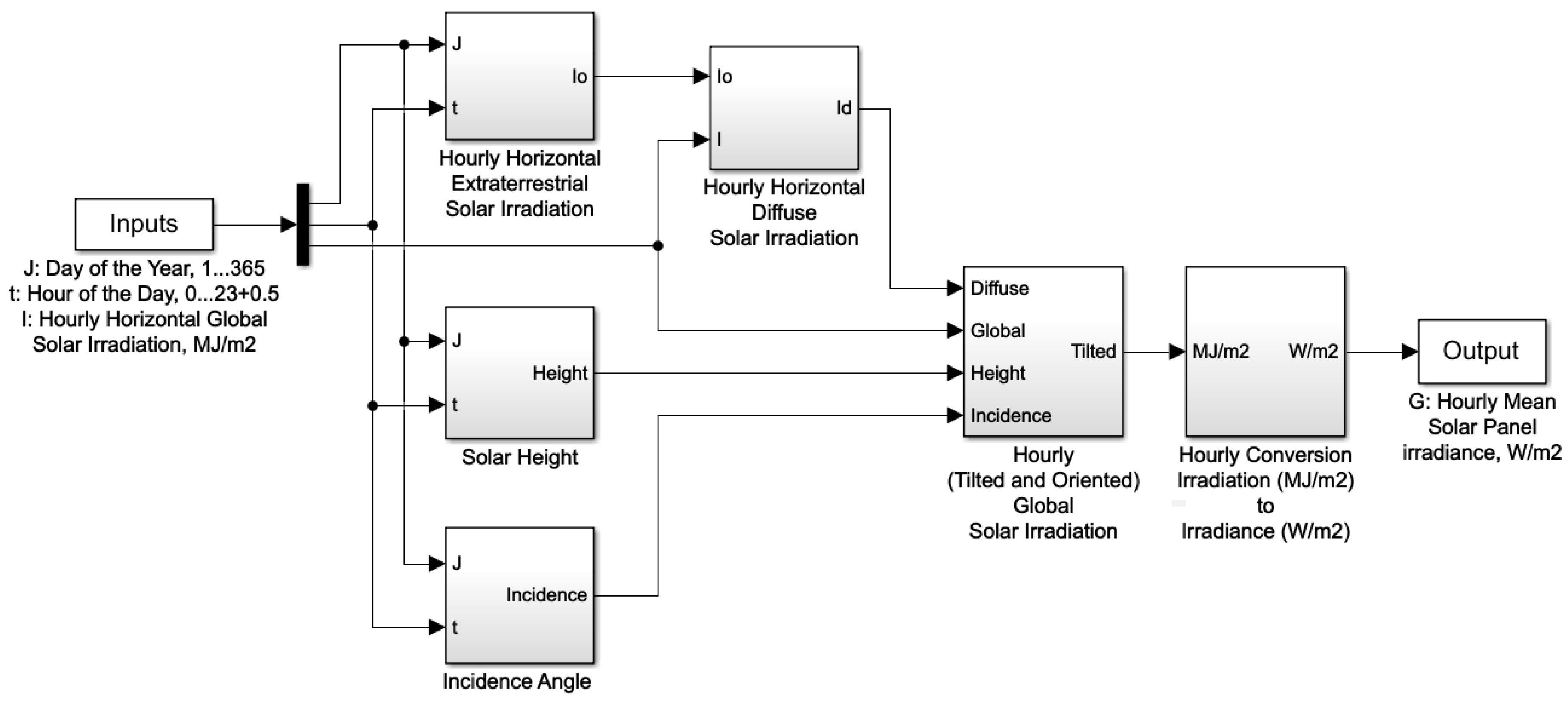
2.3. Simulink-MATLAB Methodology for Estimating the Solar Irradiation Incident on the Inclined Plane

For the calculation of solar irradiation on an inclined and/or oriented surface, existing models described in the literature need the horizontal global solar irradiation, horizontal diffuse solar irradiation, solar height, and angle of incidence as input variables, with their values either measured or estimated. When other models are used for the calculation (e.g., horizontal diffuse solar irradiation), the value of extraterrestrial solar irradiation is provided through parameters such as the solar constant, a correction factor for Earth’s eccentricity, the day of the year, the solar declination, and the solar time angle, as well as others pertaining to the location of the greenhouse, such as its geographical latitude and longitude, and the inclination and orientation of the solar panels.

In this study, the methodology was developed with models from different authors that have been accepted in the literature; however, to facilitate its use, the Simulink-MATLAB platform for programming with visual objects was deployed. The modular nature of its design provides the possibility of using different existing models for different case studies, depending on which is the most suitable, or creating new models to obtain the various variables required.

In this study, the value of the hourly global solar irradiation on an inclined plane, according to the scheme proposed in Figure 1, was calculated with six functional blocks:

−

a block for calculating the hourly extraterrestrial solar irradiation on the horizontal surface, I₀;

−

a block for calculating the solar height, α, for each hour of the day;

−

a block for calculating the angle of incidence, Ѳ, of the solar rays on the inclined and/or oriented plane;

−

a block for estimating the diffuse solar irradiation of the hourly sky on the horizontal surface, I_d;

−

a block for the union of the three components on the inclined plane;

−

a block for the conversion of irradiance to hourly mean solar irradiance.

This methodology received the following as input variables:

−

the day of the year, J (i.e., 1 for January 1,…, 365 for December 31);

−

the mean value of the hourly interval to study, t (i.e., the time of day + 0.5);

−

the hourly global solar irradiation measured on the horizontal surface, I.

The rest of the parameters were set inside each block and identified the position of the solar panels of the photovoltaic system and the location of the greenhouse:

−

the inclination of the solar panel, β;

−

the orientation of the solar panel, γ;

−

the solar constant, I_sc;

−

the albedo, ρ;

−

the latitude, the geographical φ of the greenhouse;

−

the geographical longitude of the greenhouse.

The following sections detail the implementation of each block of the methodology developed in Simulink-MATLAB.

2.3.1. Hourly Extraterrestrial Solar Irradiation Block

The Sun emits a flow of energy which is considered to be almost constant except for small variations due to sun spots. This solar energy, when it reaches the top of the atmosphere, receives the name of extraterrestrial solar irradiation and it is this solar irradiation that would reach a certain point on Earth if the atmosphere that protects it did not exist.

Extraterrestrial solar irradiation for various latitudes can be estimated from the following parameters: the solar constant, the solar declination, and the time of year. For hourly or shorter periods, the solar angle at the beginning and the end of the period has to be considered (see the work of Allen [40], recommended by the FAO for the development of calculations for crop evapotranspiration, Duffie et al. [41], and Kalogirou [42]). This is done with Equation (13).

$${\mathrm{I}}_0=\left(\frac{12·60}{\mathsf{\pi }}\right){\mathrm{I}}_{\mathrm{sc}}{\mathrm{E}}_0\left[\left({\mathsf{\omega }}_2-{\mathsf{\omega }}_1\right)\mathrm{sen}\mathsf{\varphi }\mathrm{sen}\mathsf{\delta }+\cos \mathsf{\varphi } \cos \mathsf{\delta }\left({\mathrm{sen}\mathsf{\omega }}_2-{\mathrm{sen}\mathsf{\omega }}_1\right)\right]$$

(13)

where:

• I₀: hourly extraterrestrial solar irradiation incident on a horizontal surface, MJ/(m²·h);
• I_sc: solar constant, 0.082 MJ/(m²·min);
• E₀: correction factor for the eccentricity of the Earth (r₀/r)², with E₀ = 1 + (0.033·cos(2·π·J/365));
• r₀: average Sun–Earth distance, 1 ua;
• r: current Sun–Earth distance, ua;
• ua: astronomical unit, 1496 × 10⁸ km;
• J: day number of the year, 1 for January 1, …, 365 for December 31;
• ϕ: geographic latitude (rad), north (+) and south (−): −90° ≤ ϕ ≤ 90° where (rad) = π/180·(°decimal places);
• δ: solar declination (rad), with δ = 0.409·sen((2·π·J/365) − 1.39). Defined as the angular position of the Sun at solar noon—that is, when the Sun is in the local meridian—in relation to the plane of the Earth’s equator, north (+) and south (−): −23.45° ≤ $\mathsf{\delta }$ ≤ 23.45°;
• ω₁: solar hour angle at the beginning of the period (rad), with ω₁ = ω − ((π·t₁)/24);
• ω: solar hour angle at the moment when the midpoint of the considered period occurs (rad), with ω = (π/12)·[(t + 0.06667·(L_z − L_m) + S_c) − 12];
• t₁: duration of the period considered (hours), 1 for hourly periods, 0.5 for periods of 30 min;
• t: standard time at the midpoint of the period considered (hours) (e.g., for a period between 2:00 p.m. and 3:00 p.m., t = 14.5);
• L_z: geographic longitude of the center of the local time zone, degrees west of Greenwich: 75° East, 90° Central, 105° Rocky Mountain, 120° Pacific USA, 0° Greenwich, 330° Cairo, 255° Bangkok, 345° Spain (Iberian Peninsula);
• L_m: geographic longitude of the measurement area, degrees west of Greenwich;
• S_c: seasonal correction for solar time (hours), with S_c = 0.1645·sen(2b) − 0.1255·cos(b) − 0.025·sen(b) and b = 2·π·(J − 81)/364;
• ω₂: solar hour angle at the end of the period (rad), with ω₂ = ω + ((π·t₁)/24). If, in the morning, ω < −ω_s, or, in the afternoon, ω > ω_s, this indicates that the Sun is below the horizon such that I₀ = 0.

It is necessary to take into account the advance of the clock time in the official time (i.e., wintertime UTC+1 from the last Sunday in October and summertime UTC+2 from the last Sunday in March).

2.3.2. Horizontal Diffuse Solar Irradiation Block

The horizontal diffuse solar irradiation modeling from the hourly clearness index (k_t = I/I₀) and an hourly diffuse fraction (k_d = I_d/I) was carried out with a third-order model (that of Miguel et al. [43]) and was performed using data from several countries in the northern Mediterranean, resulting in Equation (14).

$${\mathrm{k}}_{\mathrm{d}}=\{\begin{array}{l}0.995-0.081{\mathrm{k}}_{\mathrm{t}}\hfill \\ 0.724+2.738{\mathrm{k}}_{\mathrm{t}}-8.32{\mathrm{k}}_{\mathrm{t}}^2+4.967{\mathrm{k}}_{\mathrm{t}}^3\hfill \\ 0.18\hfill \end{array}\mathrm{for}\begin{array}{l}{\mathrm{k}}_{\mathrm{t}}\le 0.21\hfill \\ 0.21<{\mathrm{k}}_{\mathrm{t}}\le 0.76\hfill \\ 0.76<{\mathrm{k}}_{\mathrm{t}}\hfill \end{array}$$

(14)

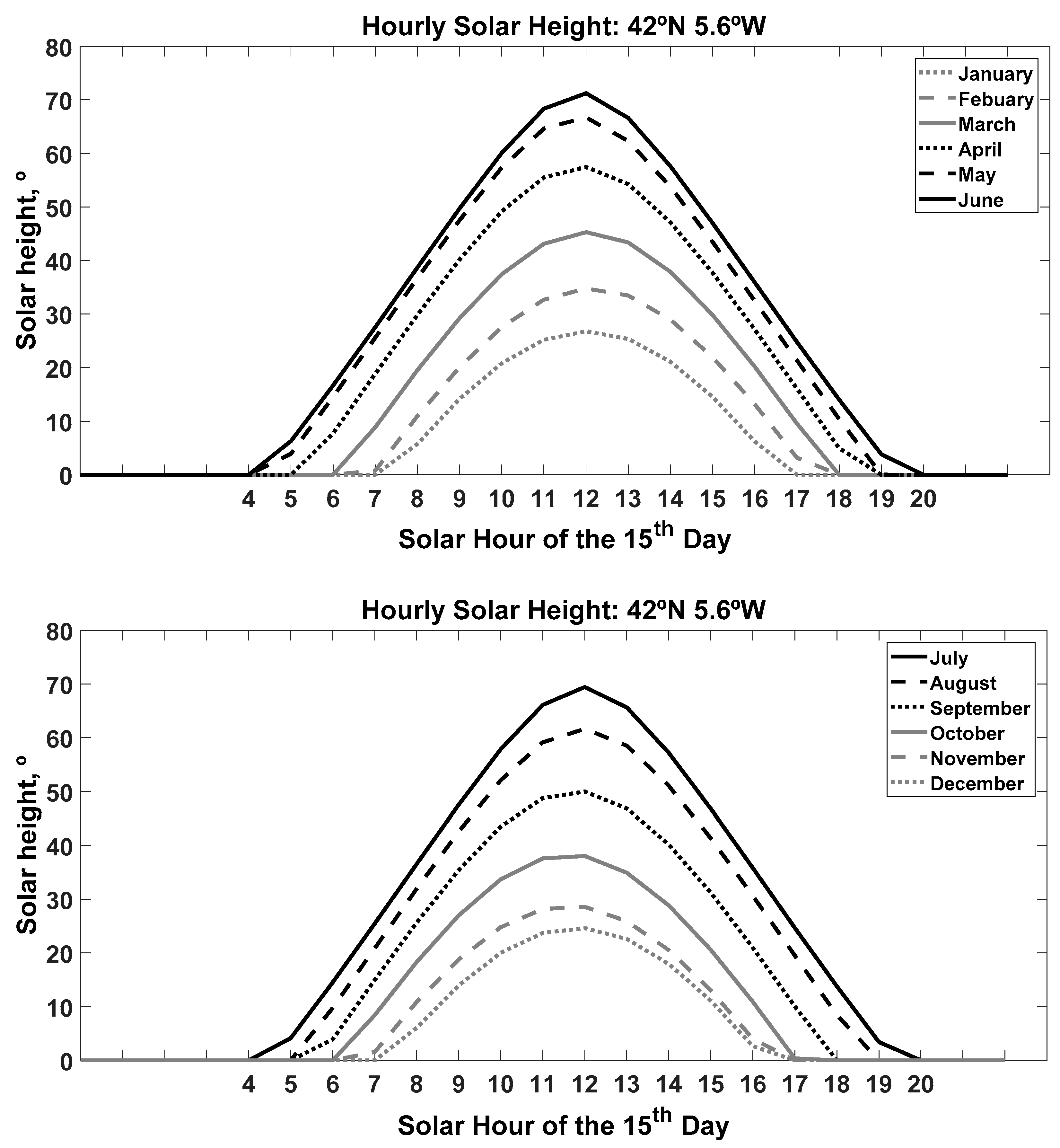
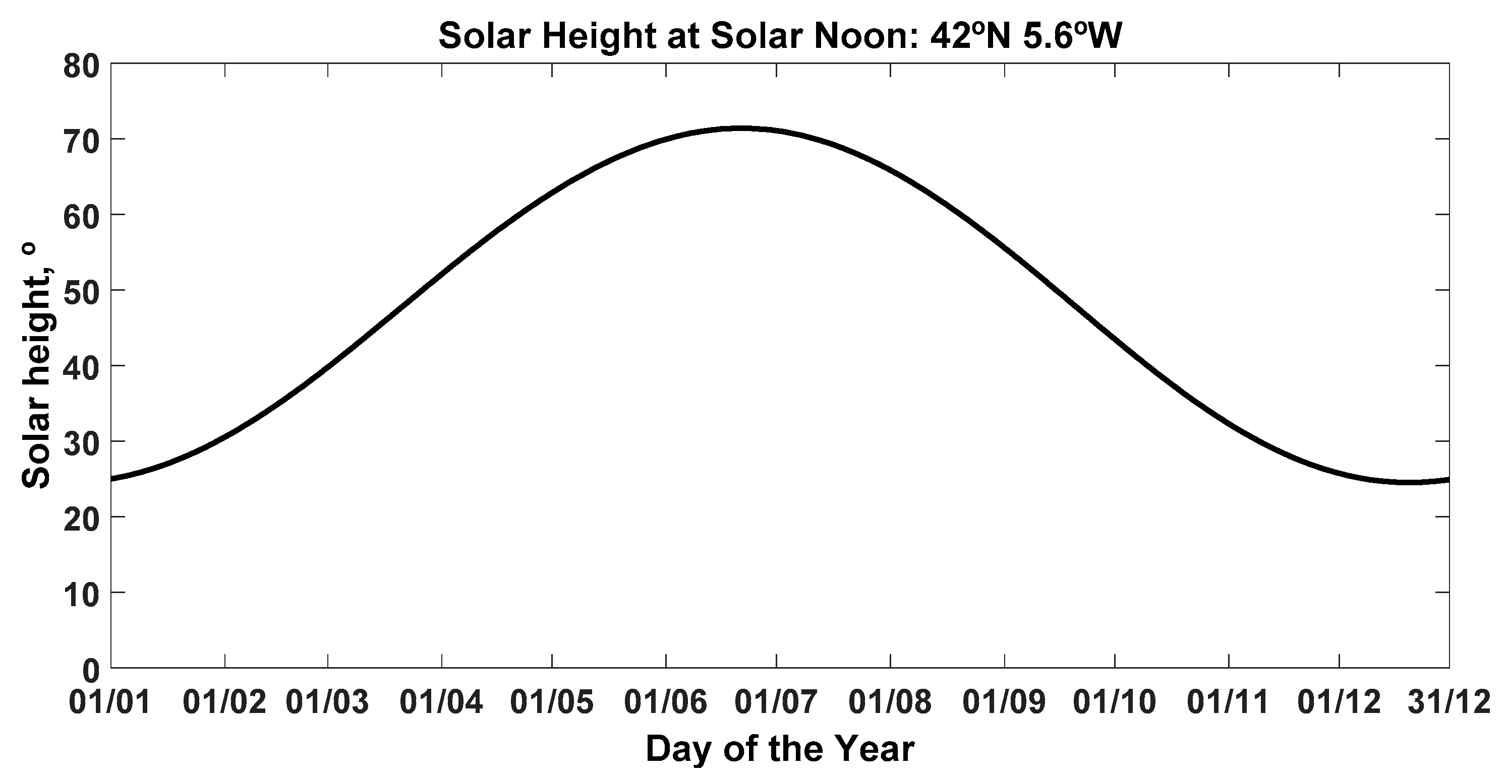
2.3.3. Solar Height and Zenith Angle Block

Solar height, also called solar elevation, is the angular height of the Sun above the observer’s celestial horizon, which is an angle between 0° and 90°. The zenith angle, also called the zenith distance, is the angle between the local zenith and the line that joins the observer and the Sun; the value of the angle is between 0° and 90°. The solar height is the complement of the zenith angle. For a given geographic position, in the absence of atmospheric refraction of the earth, the trigonometric relationship between the Sun and a horizontal surface provided by Iqbal [35] is defined by Equation (15).

$$\cos {\mathsf{\theta }}_{\mathrm{z}}=\mathrm{sen}\mathsf{\delta }\mathrm{sen}\mathsf{\varphi }+\cos \mathsf{\delta }\cos \mathsf{\varphi }\cos \mathsf{\omega }=\mathrm{sen}\mathsf{\alpha }$$

(15)

where:

• $\mathsf{\alpha }$: solar height—the angle of elevation of the Sun above the true horizon;
• ${\mathsf{\theta }}_{\mathrm{z}}$: zenith angle—the angular position of the Sun in relation to the local vertical, ${\mathsf{\theta }}_{\mathrm{z}}$ = 90° − $\mathsf{\alpha }$.

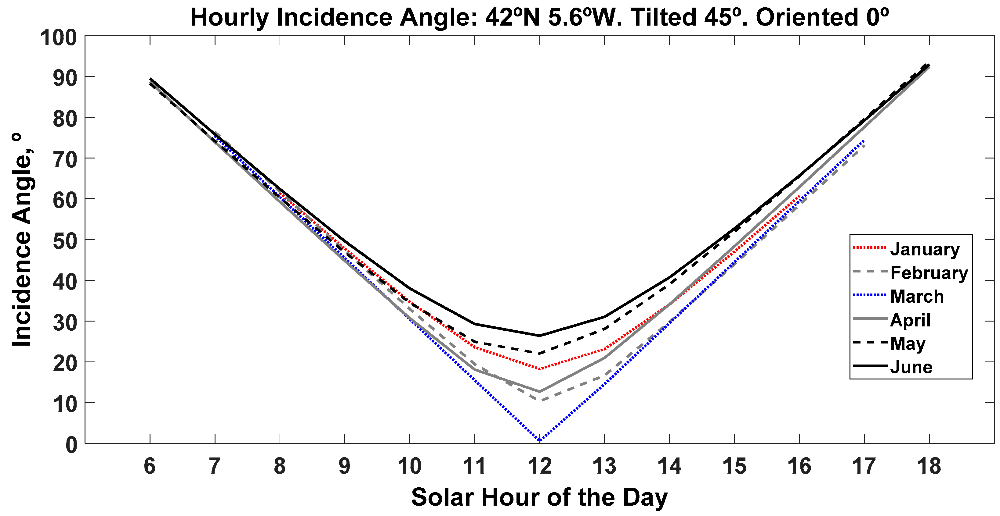
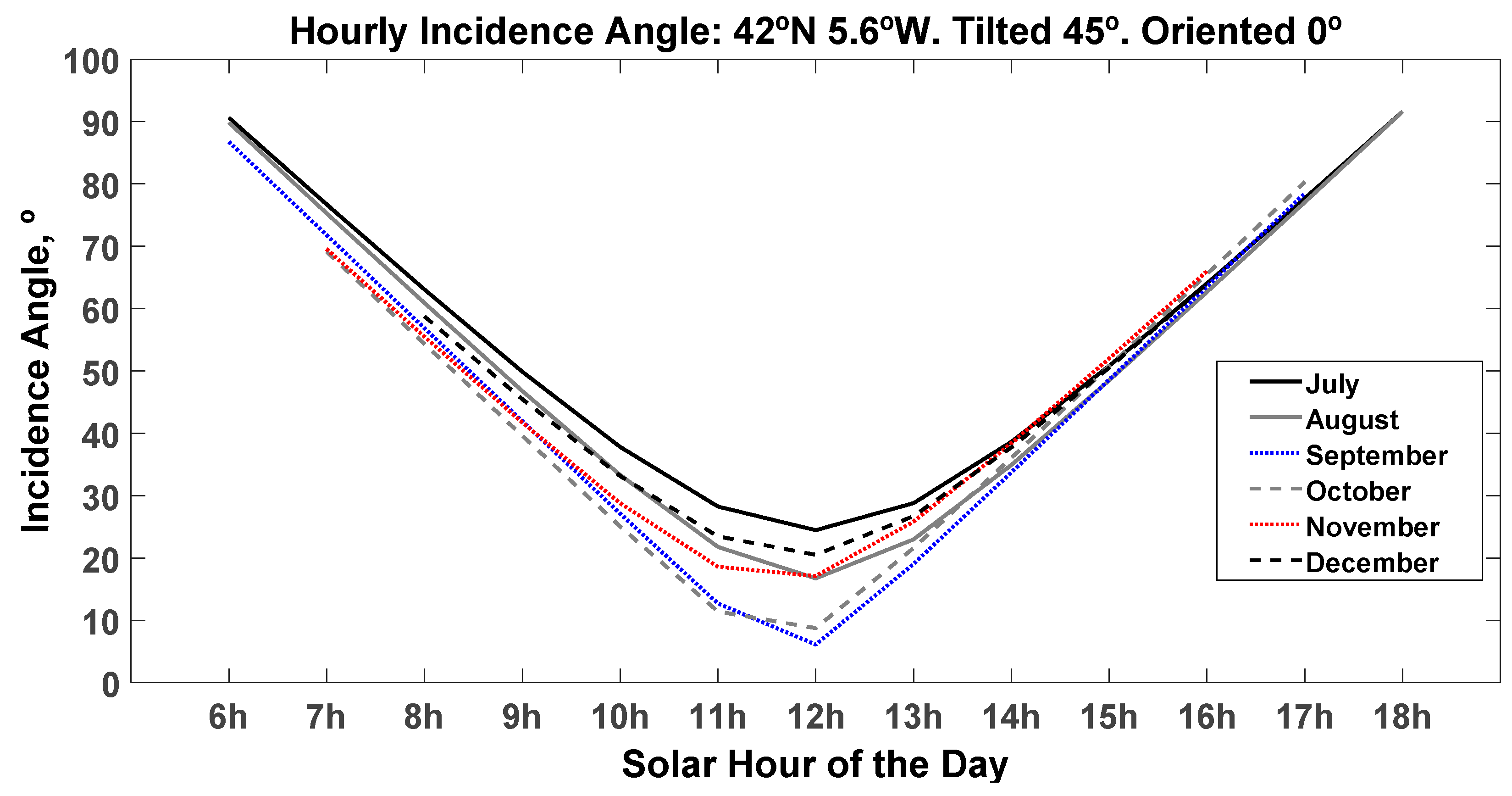
2.3.4. Angle of the Incidence of Solar Irradiation on the Solar Panel Block

The angle of incidence is the angle formed between the normal to the inclined plane and the Sun–Earth vector. There are two cases: the inclined plane may be oriented towards the equator or with an arbitrary orientation towards east or west.

−

Modeling the angle of incidence for an inclined solar panel oriented towards the equator

The angle of incidence for an inclined surface oriented towards the equator can be described, as detailed by Liu and Jordan [12], with Equation (16).

$$\cos {\mathsf{\theta }}_0=\mathrm{sen}\mathsf{\delta }\mathrm{sen}\left(\mathsf{\varphi }-\mathsf{\beta }\right)+\cos \mathsf{\delta }\cos \left(\mathsf{\varphi }-\mathsf{\beta }\right)\cos \mathsf{\omega }$$

(16)

where:

• ${\mathsf{\theta }}_0$: angle of incidence for an inclined surface oriented towards the equator;
• $\mathsf{\beta }$: inclination of the surface to the horizontal position.

−

Modeling the angle of incidence for an arbitrarily inclined and oriented solar panel

The relationship of the angle of incidence for a surface inclined and oriented in any direction with the local meridian is trigonometric (see Berod and Bock [44], Kondratyev [45], and Coffari [46]) and can be described with Equations (17) or (18).

$$\begin{array}{ll}\cos \mathsf{\theta }=& \left(\mathrm{sen}\mathsf{\varphi }\cos \mathsf{\beta }-\cos \mathsf{\varphi }\mathrm{sen}\mathsf{\beta }\cos \mathsf{\gamma }\right)\mathrm{sen}\mathsf{\delta }\\ & +\left(\cos \mathsf{\varphi }\cos \mathsf{\beta }+\mathrm{sen}\mathsf{\varphi }\mathrm{sen}\mathsf{\beta }\cos \mathsf{\gamma }\right)\cos \mathsf{\delta }\cos \mathsf{\omega }\\ & +\cos \mathsf{\delta }\mathrm{sen}\mathsf{\beta }\mathrm{sen}\mathsf{\gamma }\mathrm{sen}\mathsf{\omega }\end{array}$$

(17)

where:

• $\mathsf{\theta }$: the angle of incidence for an arbitrarily inclined and oriented surface.

$$\cos \mathsf{\theta }=\cos \mathsf{\beta }\cos {\mathsf{\theta }}_{\mathrm{z}}+\mathrm{sen}\mathsf{\beta }\cos {\mathsf{\theta }}_{\mathrm{z}}\cos \left(\mathsf{\psi }-\mathsf{\gamma }\right)$$

(18)

where:

• $\mathsf{\gamma }$: azimuth angle of the surface, orientation. Defined as the deviation of the normal to the surface of the solar collector from the local meridian in the directions west (−), south (0), and east (+);
• $\mathsf{\psi }$: solar azimuth with cosψ = ((senα·senϕ-senδ)/(cosα·cosϕ)), with 0° ≤ ψ ≤ 90° for cosψ ≥ 0, and with 90° ≤ ψ ≤ 180° for cosψ ≤ 0. This is the angle at the local zenith between the plane of the observer’s meridian and the plane of a great circle passing through the zenith and the Sun in the directions west (−), south (0), and east (+): −180° ≤ 0° ≤ +180°.

Measurement of the angle of incidence of the direct solar irradiation can be done by constructing a simple device. This consists of mounting a normal pointer to a flat surface, on which graduated concentric circles are marked. The length of the shadow cast by the pointer can be measured using concentric circumferences and can be used to determine the angle of incidence according to the international standard ISO 9806:2017 [47]. The device should be located on the plane and to one side of the solar panel.

2.3.5. Angle of the Incidence of the Solar Irradiation on the Solar Panel Block

This block was used to unify the three components of solar radiation that affect the solar panel in order to obtain the amount of the global solar radiation incident on the inclined surface.

2.3.6. Conversion from Hourly Global Irradiance to Hourly Mean Solar Irradiance Block

Finally, the conversion of the global hourly solar irradiance (i.e., energy value) obtained for the inclined and oriented plane to the corresponding hourly mean solar irradiance (i.e., power value) was undertaken. Through interpolation, these hourly values can be used to create a database with a time interval of one minute in order to carry out a more detailed simulation of the operation of the photovoltaic system under study (e.g., as input values for the simulation of a model of a greenhouse photovoltaic system).

3. Results

This section presents the results of the selected models for the estimation of the global solar irradiation value on the solar panel inclined plane, based on the global solar irradiation on the horizontal surface (which is usually recorded in meteorological stations) and using the following Simulink-MATLAB blocks:

−

hourly extraterrestrial solar irradiation;

−

hourly horizontal diffuse solar irradiation;

−

the hourly solar height;

−

the hourly angle of incidence on the solar panel;

−

the hourly global solar irradiance and hourly average solar irradiance on the solar panel.

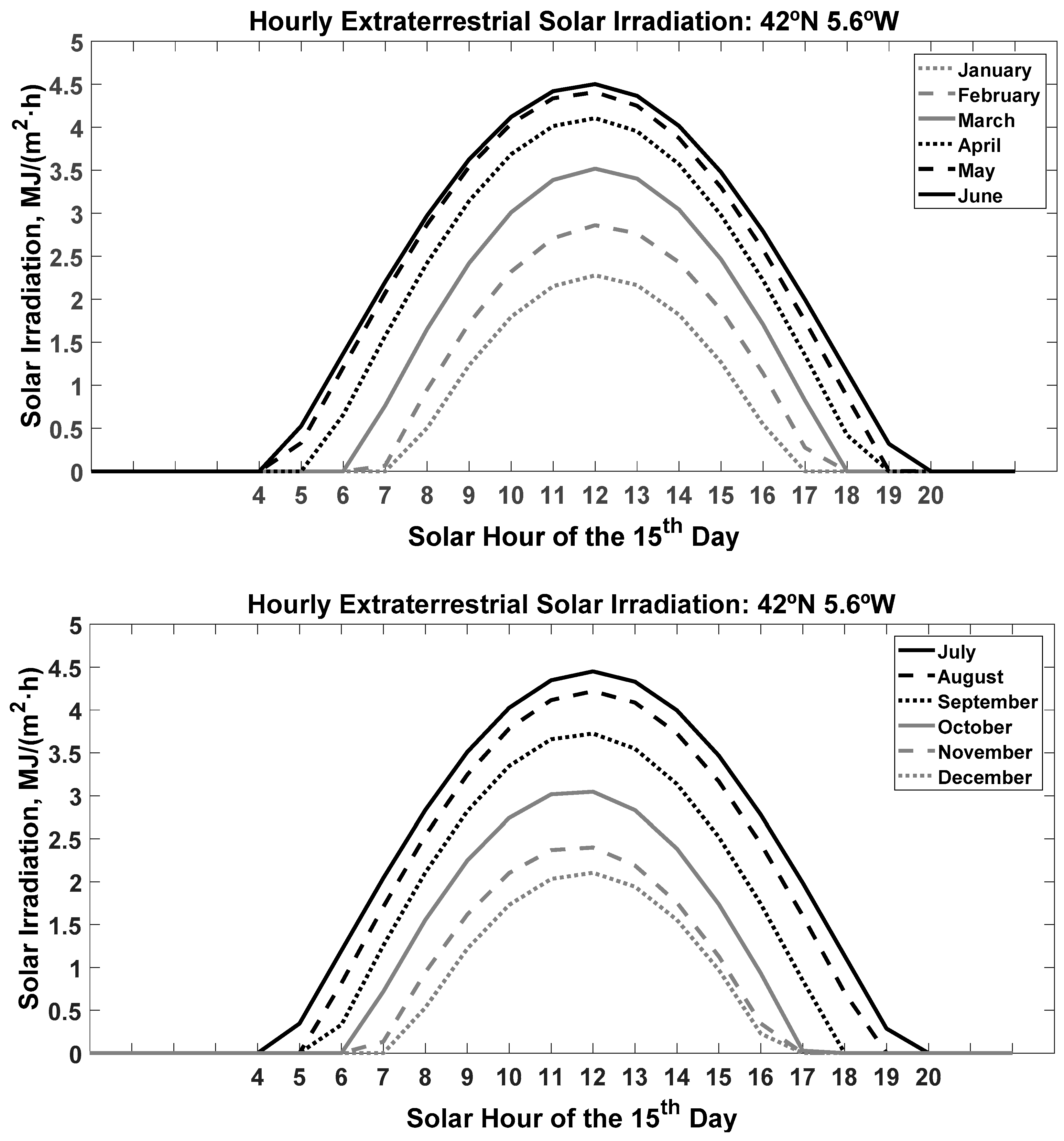
3.1. Result of the Hourly Extraterrestrial Solar Irradiation Block

The extraterrestrial solar irradiation modeling was applied to determine the temporal evolution of the extraterrestrial solar irradiation at the top of the atmosphere (which would be found to reach a certain point on Earth if the attenuation and scattering effects which are produced by the atmosphere when the sun’s rays pass through it are not considered).

The results of the methodology for the calculation of hourly extraterrestrial solar irradiation, obtained for the 15th day of each month of the year at latitude 42° N and longitude 5.6° W, are shown in (Figure 2).

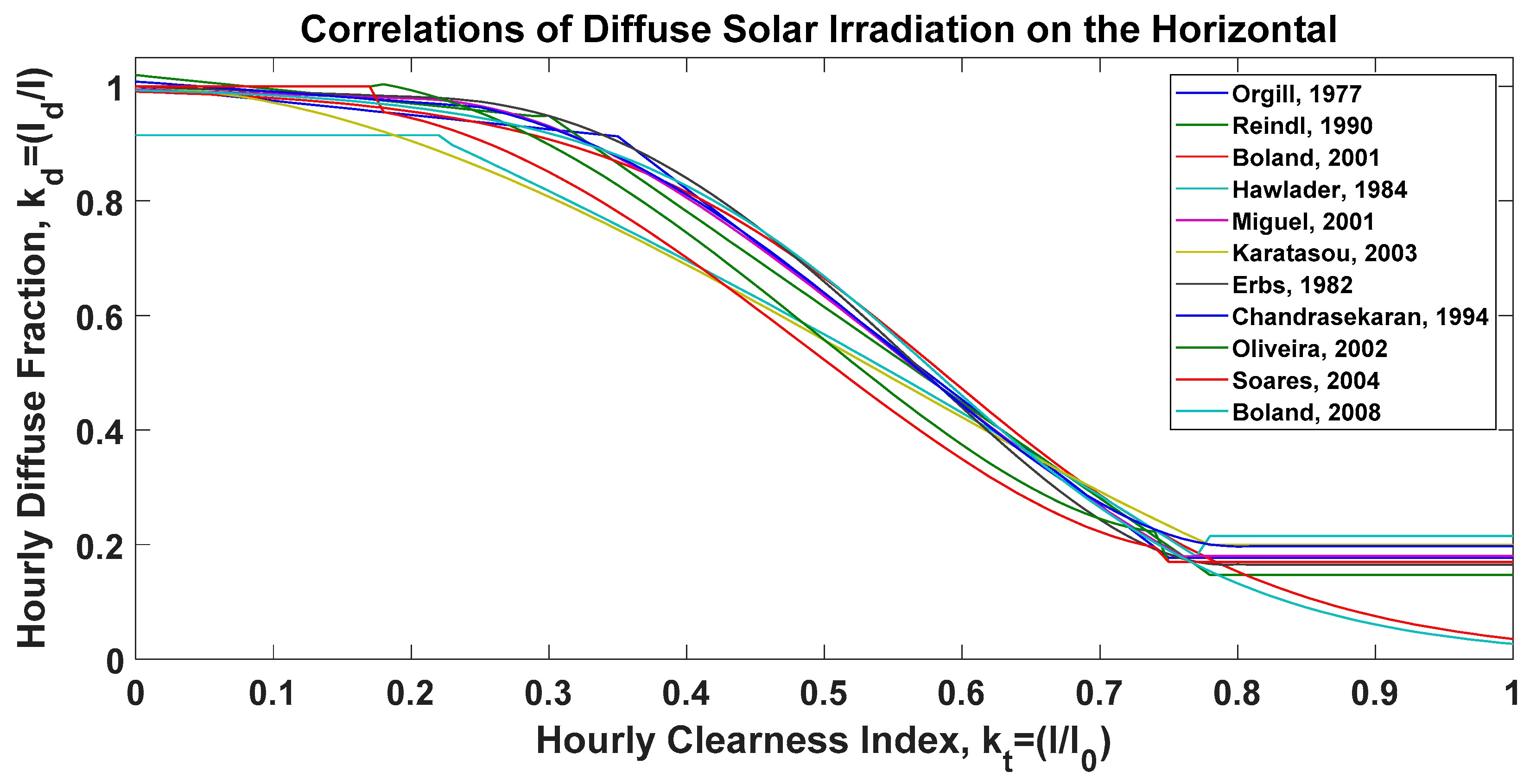
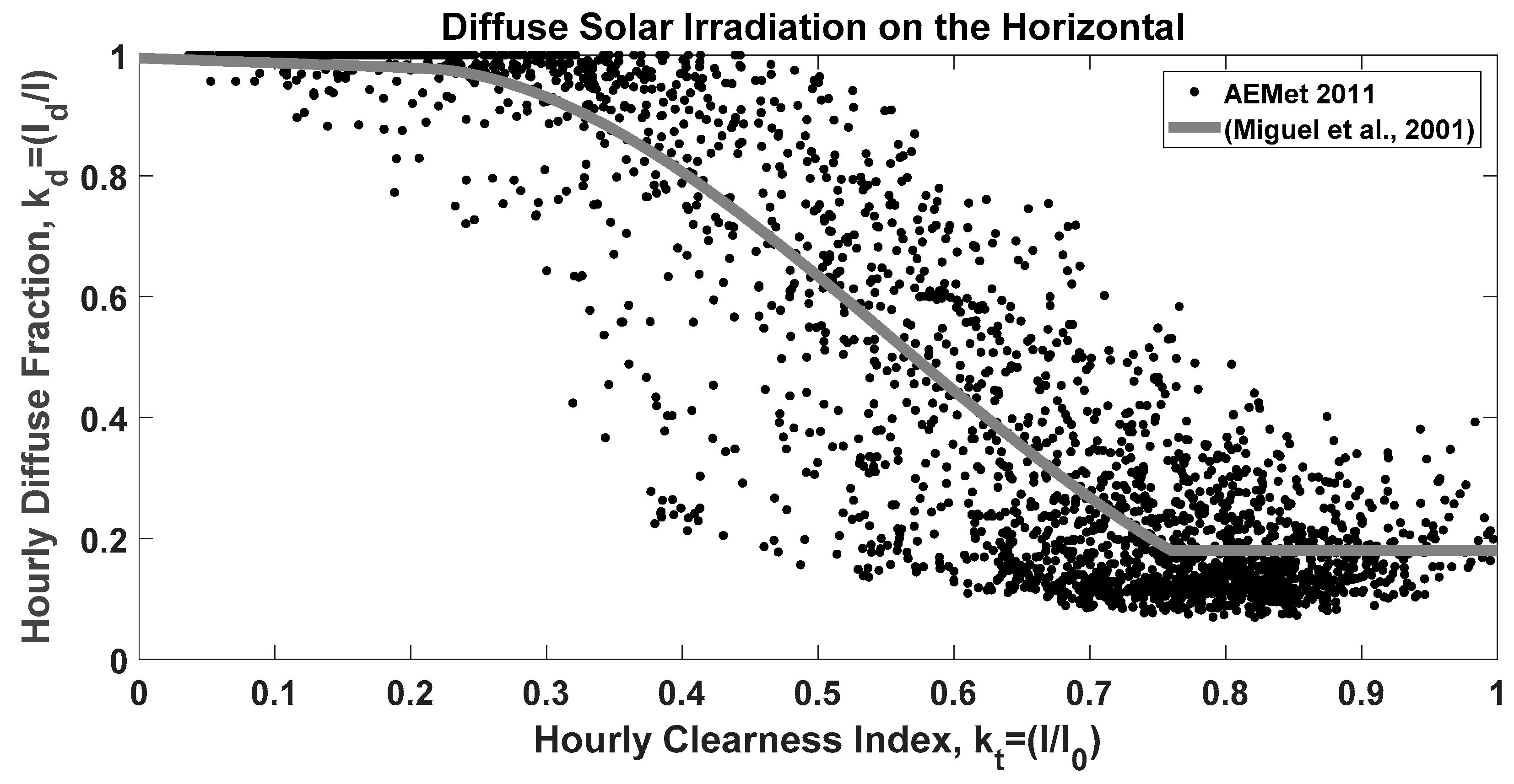
3.2. Result of the Hourly Horizontal Diffuse Solar Irradiation Block

The different correlations proposed for the hourly diffuse fraction in the introduction are shown in Figure 3. Generally, each model includes three relationships for each sky type, as detailed by Iqbal [35], that determine the daily clearness index in order to define sky conditions such that:

−

for clear sky, 0.7 ≤ k_t < 0.9;

−

for partly cloudy sky, 0.3 ≤ k_t < 0.7;

−

for overcast sky, 0 ≤ k_t < 0.3.

Figure 4 shows the results of the methodology used for the conversion of the hourly diffuse solar irradiation to the hourly global solar irradiation, using data recorded by the State Meteorological Agency (AEMet) at La Virgen del Camino station (León, Castile and León region, Spain), with regard to the relation between the hourly diffuse fraction and the hourly clearness index, with values recorded for the central eight hours of the day during 2011, along with the model selected (Miguel et al. [43]).

3.3. Result of the Hourly Solar Height Block

The results of the methodology used for the modeling of the hourly solar height, obtained for the 15th day of each month of the year at latitude 42° N and longitude 5.6° W, are shown in Figure 5.

Figure 6 shows that the maximum values for the solar height were obtained at solar midday.

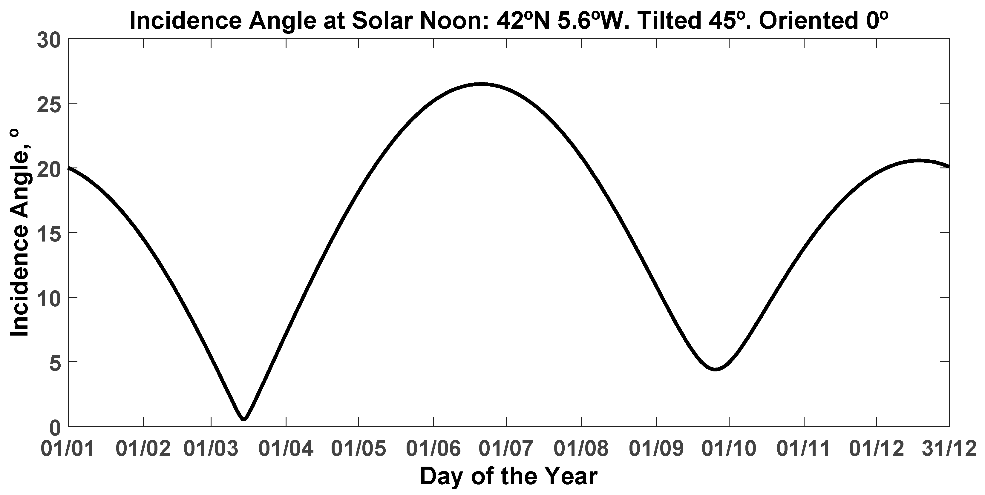
3.4. Result of the Hourly Incidence Angle Block

Figure 7 shows the results of the methodology used for the modeling of the hourly incidence angle obtained for the surface of a solar panel with an inclination of 45° and oriented towards the equator, for the 15th day of each month of the year at latitude 42° N and longitude 5.6° W.

The minimum values of the angle of incidence, which were obtained at solar noon for each day of the year, are presented in Figure 8.

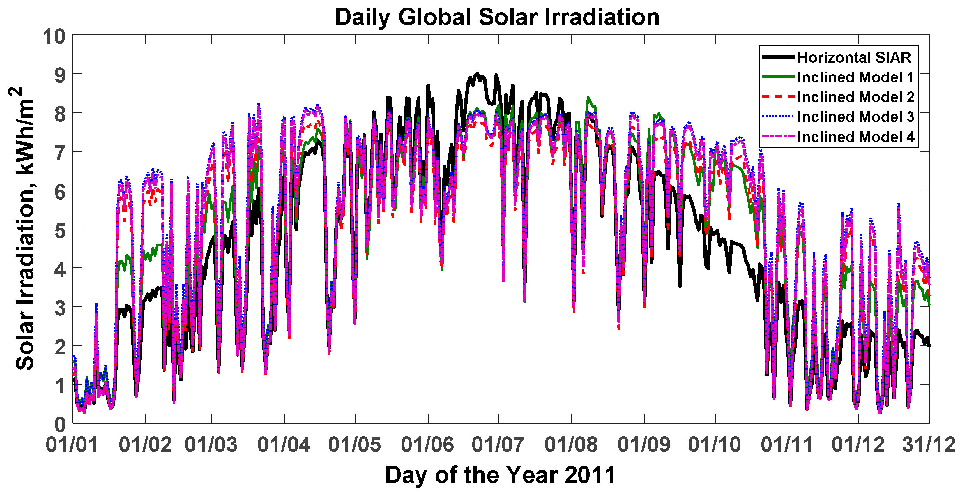
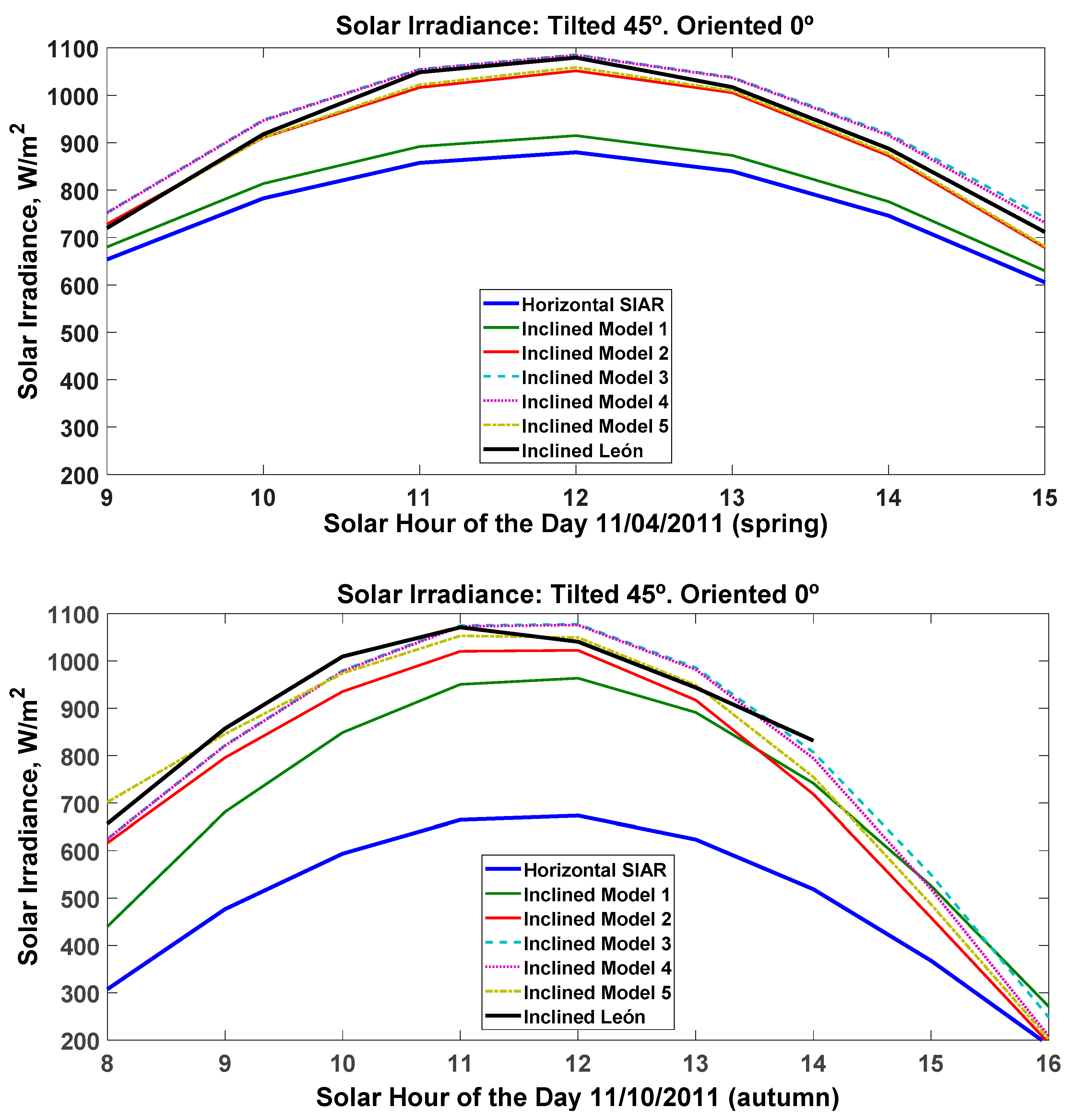
3.5. Results for Hourly Global Irradiance and Hourly Mean Solar Irradiance on the Solar Panel

The data recorded for the global solar irradiation on the horizontal surface during 2011 in the agrometeorological station located in the town of Mansilla Mayor (León, Castile and León region, Spain), as part of the SIAR network, were used to apply the methodology developed in Simulink-MATLAB for the estimation of the global solar irradiation value on a surface with an inclination of 45° and oriented towards the equator. The results of the different methods of obtaining diffuse solar irradiation are shown below.

Figure 9 shows the values of the daily global solar irradiation obtained from the horizontal SIAR network, together with the calculations carried out for the estimation of the daily global solar irradiation on a surface inclined at 45° and oriented to the equator using the following four models.

−

Inclined Model 1

Inclined Model 1 used the CENSOLAR [48] method, which provides a coefficient to obtain the value of the global solar irradiation on the solar panel, depending on the latitude, the inclination, and the month of the year.

The following models (Inclined Models 2, 3, 4, and 5) used the methodology described in the previous sections for the values of the direct component and the albedo of the solar irradiation, while different models were used for the value of the diffuse component, therefore obtaining different results.

−

Inclined Model 2

Inclined Model 2 used the Liu and Jordan isotropic model, presented in Equation (7), for the estimation of the diffuse component.

−

Inclined Model 3

Inclined Model 3 used the anisotropic model of Temps and Coulson, presented in Equation (8), for the estimation of the diffuse component.

−

Inclined Model 4

Inclined Model 4 used the Klucher anisotropic model, presented in Equation (9), for the estimation of the diffuse component.

−

Inclined Model 5

Inclined Model 5 used Hay’s anisotropic model, presented in Equation (10), to estimate the diffuse component.

Finally, the conversion module was applied to convert the global hourly solar irradiance values, given in energy units (MJ/m²), on the inclined plane into the average hourly values of the solar irradiance, given in power units (W/m²), on the inclined plane.

In Figure 10, the hourly variation of the solar irradiance is represented for one day in April (spring) and another day in October (autumn) in order to compare the solar irradiance on the inclined plane calculated with the five conversion methods with the evolution of the data from the global horizontal solar irradiance SIAR located in Mansilla Mayor (León, Castile and León region, Spain), specifically the solar irradiance recorded by the pyranometer of the solar panel.

Table 1. Observed adjustment of the hourly solar irradiance on the plane inclined at 45° and oriented towards the equator, as estimated with Inclined Models 2, 3, 4, and 5 from data for the horizontal surface from the agrometeorological station SIAR in Mansilla Mayor (León, Castile and León, Spain), along with the values measured in León, for four days.

Day	Inclined Model 2		Inclined Model 3		Inclined Model 4		Inclined Model 5
	RMSE	R2	RMSE	R2	RMSE	R2	RMSE	R2
11 April 2011	21.90	0.9751	25.09	0.9674	22.14	0.9746	17.83	0.9835
1 June 2011	38.51	0.8658	32.14	0.9065	31.54	0.9100	55.12	0.7250
30 June 2011	21.40	0.9415	40.11	0.7947	39.06	0.8052	11.95	0.9817
11 October 2011	62.36	0.7853	31.44	0.9454	32.51	0.9416	37.32	0.9230

Inclined Model 2 utilized the Liu and Jordan isotropic model; Inclined Model 3 utilized the Temps and Coulson anisotropic model; Inclined Model 4 utilized the Klucher anisotropic model; Inclined Model 5 utilized the Hay anisotropic model; RMSE, root mean square error (W/m²); R², determination coefficient. The best results for each day are underlined.

lists the statistical results for four random sunny days, comparing the estimates made with the isotropic model and the three anisotropic models with the measured values for the inclined plane oriented towards the equator.

4. Discussion

Once the estimation of the solar irradiation received by the inclined solar panel has been undertaken, the results obtained were analyzed using the Simulink-MATLAB blocks (Figure 1).

For the modeling of the extraterrestrial solar irradiation, symmetry can be observed throughout the day with regard to solar noon in Figure 2, along with a progressive increase in solar irradiation for the seasonal component from December to June and a decrease in solar irradiation from June to December (41.91‒12.28 MJ/m² daily). The results were validated by comparing the sum of the hourly values of each day with those described by Allen [40] and resulted in a good approximation without the need for more statistics.

Three differentiated zones can be seen in the horizontal diffuse solar irradiation modeling (Figure 4). In one, a maximum hourly diffuse fraction (k_d) and a minimum hourly clearness index (k_t) were obtained (i.e., corresponding to the hours of the day with the sky covered); another zone was characterized by a minimum hourly diffuse fraction (k_d) and a maximum hourly clearness index (k_t) (i.e., corresponding to the hours of the day with clear skies); finally, there was a third intermediate zone with indices k_d and k_t inversely variable with each other, depending on the degree of cloudiness of the sky (i.e., corresponding to the hours of the partially cloudy day). The model provided in the study by Miguel et al. [43], which was developed in Mediterranean areas, shows a good approximation with the model obtained with the data recorded by the State Meteorological Agency (AEMet) at La Virgen del Camino station (León, Castile and León region, Spain) during the central eight hours of the day for the whole year of 2011. It can be observed that the data for clear sky days was different from the Miguel model (the mean diffuse fraction on clear days was lower than that of the Miguel model), which indicates a low dispersion of the solar irradiation of the sky on clear days (i.e., a very clear and clean sky in the place under study).

In the solar height modeling, in Figure 5 symmetry can be observed throughout the day with regard to solar noon, along with a progressive increase in solar height from December to June and a decrease in solar height from June to December. The results were validated by comparison with those described by Duffie et al. [41], showing a good approximation without the need for more statistics. The maximum values of solar height occurring at solar noon, which were observed throughout the year (Figure 6), reached their maximum during the last fortnight of June at the highest position of the Sun (72°), and the minimum solar height occurred during the last fortnight of December (24.5°).

For the results for the modeling of the angle of incidence, symmetry can be observed throughout the day with respect to solar noon, for which the minimum value was obtained, in Figure 7. In Figure 8, the progressive decrease from December to March (0.5°), the increase from March to June (26.5°), the decrease from June to September (4.5°), and the increase from September to December (20.5°) can be seen. The results were validated by comparison with those presented by Bérriz and Álvarez [49] and Duffie et al. [41], showing a good approximation without the need for more statistics. The most favorable months of the year, with the position of the solar panel inclined 45° and oriented towards the equator, for capturing solar energy were February, March, April, September, and October, as the inclined surface was in a more perpendicular position with regard to the path of the sun’s rays on those dates.

The study of the variation of the angle of incidence is very important since it provides the time of year in which the use of solar energy is maximum, according to the inclination and orientation of the solar panel. The results of this model, if compared with the profile of annual energy needs of a photovoltaic system for a particular greenhouse, offer the possibility of finding the relationship (inclination–orientation) for each time of the year in which solar capture is optimal.

In M’Sila, Algeria, Ihaddadene et al. [50] theoretically searched for the best angle of inclination (monthly, seasonally, and annually), examining the Liu and Jordan model, the circumsolar model, the Hay model, and the Reindl model as the most appropriate models. They decided to change the angle of inclination of solar conversion systems monthly by 7272.27 MJ/m², or seasonally by 7184.94 MJ/m², instead of fixing them at 6836.83 MJ/m² in order to increase the amount of energy for a year; they recommended that this be studied using hourly data.

In Beijing, China, the annual optimal tilt angle shows a downward trend (Shen et al. [51]) compared to the optimum in the 1960s (i.e., 38°); the optimal tilt angle decreased by 2° from 2011‒2015 (i.e., to 36°), caused mainly by the decrease in the direct irradiation ratio, which is highly related to atmospheric conditions (i.e., pollution that increases the proportion of diffuse irradiation and decreases the direct irradiation).

Kondratyev and Manolova [52] have stated that direct solar irradiation has been studied in detail, but diffuse and reflected solar irradiation on inclined planes are quite complicated, requiring study in relation to the distribution of the angular intensity. Therefore, special attention must be taken when selecting the most suitable diffuse irradiation model for a particular place; furthermore solar panels are more sensitive to electrical energy conversion in photovoltaic systems than solar collectors in thermal systems.

In light of these points, in this study, different models of diffuse irradiation were analyzed for a specific place where a greenhouse is located, taking into account that the diffuse solar irradiation of the sky that falls upon the inclined plane of the solar panel is estimated in a different way as a function of the model. The circumsolar model overestimated it in Equation (6); the isotropic model underestimated it on the opposite slope of the inclined surface in Equation (7); and in clear and partly cloudy sky conditions, which occur in many cases, the light of the sky is anisotropic, meaning that the Temps and Coulson model provided a good prediction for the clear sky in Equation (8) but overestimated the solar irradiance when used for the cloudy sky. In this case, the Klucher model made corrections by setting factor F to 0 when the sky was completely cloudy in Equation (9), thus returning to the isotropic model, and setting F to 1 when the skies were, resulting in the Temps and Coulson model; this improved the estimates for all types of the sky.

In Nakhon Pathom and Ubon Ratchathani, Thailand, Wattan and Janjai [53] investigated the performances of 14 models in estimating hourly diffuse solar irradiation on inclined (30°, 60°, and 90°) and oriented (north, south, east, and west) surfaces at two tropical sites, finding that the Muneer and Gueymard models performed better.

In Algiers and Ghardaia, Algeria, and Málaga, Spain, Takilalte et al. [54] estimated the inclined global irradiation in 5-min intervals, using global irradiation on the horizontal plane, geographical parameters, site albedo, and two cloudiness factors, based on a combination of two models (Perrin Brichambaut and Liu and Jordan) for which the parameters of the state of the sky transformed the isotropic models into an anisotropic model. The results of the proposed model for all sky conditions with regard to the normalized root mean square error (nRMSE), the relative percentage error (RPE), the normalized mean absolute error (nMAE), and the correlation coefficient (R²) varied between 4.70–6.41%, 5.50–5.90%, 3.07–4.73%, and 0.97–0.99, respectively, which are very accurate results, especially for such short time scales in which there is no compensation or average effects, as occur when using monthly data.

Putting the three solar irradiation components together using Equation (11), with the solar panel at an inclination of 45° and oriented towards the equator, differences with regard to the incident on the horizontal surface shown in Figure 9 were observed according to the time of year:

−

it was higher in the months of average solar irradiation (i.e., February, March, April, September, October, and November) because then the solar height produces a lower angle of incidence on the solar panel than in other months;

−

it was moderate in the months of high solar irradiation (i.e., May and August);

−

it was lower in the months of very high solar irradiation (i.e., June and July) due to the high solar height.

In Athens, Greece, Raptis et al. [55] studied the ideal inclination to maximize the capture of solar irradiation, which was determined by the latitude and the time of year, with the horizontal surface receiving more irradiance than the inclined surface during the summer months and on cloudy winter days, due in this case to an anisotropy of the diffuse light, with a greater diffuse contribution coming from angles closer to the zenith; however, the inclined surface reached higher values than the horizontal one in winter, with the optimum angle found to be around 30° during the year.

The result of the comparison of the recorded measurements of solar irradiance on the horizontal surface (i.e., the SIAR data) and the inclined plane of the solar panel (i.e., the pyranometer in León) with the results obtained with Inclined Models 1, 2, 3, 4, and 5 (Figure 10) show a better approximation with the anisotropic models for four random sunny days. Specifically: Inclined Model 5, which used the Hay corrections, obtained better results on 4 November 2011 and 30 June 2011 with regard to the RMSE (17.83 and 11.95 W/m²) and R² (0.9835 and 0.9817), respectively. Inclined Model 4, which used the Klucher corrections, performed best on 6 January 2011, with RMSE = 31.54 W/m² and R² = 0.9100. Inclined Model 3, which used Temps and Coulson corrections, obtained better results on 10 November 2011, with RMSE = 31.44 W/m² and R² = 0.9454.

The solar panel global solar irradiation for 2011 was 1.84 MWh/m² with the CENSOLAR model, which used coefficients; 1.84 MWh/m² for the Liu and Jordan model; 1.99 MWh/m² for the Temps and Coulson model; 1.93 MWh/m² for the Klucher model; and 1.86 MWh/m² for the Hay model.

The global solar irradiation for the horizontal SIAR measured in Mansilla Mayor (León, Castile and León region, Spain) during 2011 was 1.67 MWh/m², thus resulting in a higher value on the solar panel using corrections of 10.17% for the model by Liu and Jordan, 19.16% for the Temps and Coulson model, 15.56% for the Klucher model, and 11.37% for the Hay model. However, this was distributed throughout the year, as shown in Figure 9, and as mentioned previously, was higher in the months with moderate solar irradiation (i.e., February, March, April, September, October, and November), moderate in high solar irradiation months (i.e., May and August), and lower in the months with very high solar irradiation (i.e., June and July).

In Adrar, Algeria, an increment in the performance of horizontally placed solar panels was achieved by Bailek et al. [56] with a fixed inclination of 20.61% monthly, 19.58% seasonally, 19.24% semi-annually, and 13.78% for annual adjustments, with the optimal tilt angles in each period.

5. Conclusions

Glasshouses are agricultural productive structures intended to increase the production and quality of early bloomer crops. They can be energetically characterized as follows:

• they involve intensive use of soil and means of production, which requires a safe provision of all the supplies, including energy;
• any of them are located in off-grid rural areas, so they need an autonomous energy supply;
• they are located in open areas, with great availability of solar resources and time synchronization between the supply (i.e., the Sun) and the demand (i.e., ventilation, cooling, and ferti-irrigation).

Thus, distributed generation PV systems are ideal for connection to glasshouses, either on their own or together with power generators where the value of the solar irradiance which falls upon the solar panels is the main variable to determine the performance of the PV system.

The literature pertaining to the estimation of the incidental solar irradiance on the solar panel plane (at an angle and/or oriented) in relation to the irradiance received on the horizontal surface (data registered in meteorological stations) is highly diverse, especially with regard to the types of sky in particular places. However, the practical use of this diverse information is complex, which is what incentivized the present work, in which the following methodology was adopted.

• Measured data of incidental solar irradiance on the horizontal surface in an agrometeorological station was used to obtain an estimation of the incidental solar irradiance on the plane of the glasshouse solar panels, where the verification pyranometer was located.
• A flexible methodology was built with Simulink-MATLAB software blocks that could be adapted to the numerous existing models in the literature.
• The application of components (beam, diffuse, and ground-reflected) was provided in order to ensure the use of the most adequate model for each type of sky in each location.
• Irradiance on the solar panel was obtained with an hourly resolution for various days of the year and hours of the day, along with the hourly horizontal global solar irradiance, with the location coordinate fixed. This temporal resolution is more adequate for use in the simulation of PV systems.
• The results obtained with models of diffuse anisotropic irradiance improved on those obtained with other models. As they are estimations on an hourly scale, when using data from stations close to the greenhouse, differences were observed for a few hours in the comparisons (e.g., at 12 h and 13 h on 10 November 2011 (autumn)), which may have been due to some cloudiness or changes in the reflections of the surrounding light.

As a final conclusion to this paper, it should be noted that the solar estimation for the inclined plane can be used together with the daily prediction of solar irradiance, as detailed by Diez et al. [57], to obtain the value of available solar energy in the glasshouse PV system and thus to enable more efficient management of the glasshouse electric demand.

References

1. Pérez-Alonso, J.; Pérez-García, M.; Pasamontes-Romera, M.; Callejón-Ferre, A.J. Performance analysis and neural modelling of a greenhouse integrated photovoltaic system. Renew. Sustain. Energ. Rev. 2012, 16, 4675–4685. [Google Scholar] [CrossRef]
2. Yano, A.; Cossu, M. Energy sustainable greenhouse crop cultivation using photovoltaic technologies. Renew. Sustain. Energ. Rev. 2019, 109, 116–137. [Google Scholar] [CrossRef]
3. Chaurey, A.; Kandpal, T.C. Assessment and evaluation of PV based decentralized rural electrification: An overview. Renew. Sustain. Energy Rev. 2010, 14, 2266–2278. [Google Scholar] [CrossRef]
4. Qoaider, L.; Steinbrecht, D. Photovoltaic systems: A cost competitive option to supply energy to off-grid agricultural communities in arid regions. Appl. Energy 2010, 87, 427–435. [Google Scholar] [CrossRef]
5. Cai, W.; Li, X.; Maleki, A.; Pourfayaz, F.; Rosen, M.A.; Nazari, M.A.; Bui, D.T. Optimal sizing and location based on economic parameters for an off-grid application of a hybrid system with photovoltaic, battery and diesel technology. Energy 2020, 201, 117480. [Google Scholar] [CrossRef]
6. Al-Ibrahim, A.; Al-Abbadi, N.; Al-Helal, I. PV greenhouse system—System description, performance and lesson learned. In Proceedings of the International Symposium on Greenhouses, Environmental Controls and In-house Mechanization for Crop Production in the Tropics and Sub-Tropics, Cameron Highlands, Pahang, Malaysia, 30 June 2006; Rukunuddin, K., Hamid, A., Eds.; ISHS: Leuven, Belgium, 2006; Volume 710, pp. 251–264. [Google Scholar]
7. Brooks, D.R. Bringing the Sun down to Earth: Designing Inexpensive Instruments for Monitoring the Atmosphere; Springer: New York, NY, USA, 2008. [Google Scholar]
8. Vignola, F.; Michalsky, J.; Stoffel, T. Solar and Infrared Radiation Measurements, 2nd ed.; CRC Press/Taylor & Francis Group: Boca Raton, FL, USA, 2020. [Google Scholar]
9. Hafez, A.Z.; Soliman, A.; El-Metwally, K.A.; Ismail, I.M. Tilt and azimuth angles in solar energy applications—A review. Renew. Sustain. Energ. Rev. 2017, 77, 147–168. [Google Scholar] [CrossRef]
10. Darhmaoui, H.; Lahjouji, D. Latitude based model for tilt angle optimization for solar collectors in the Mediterranean Region. Energy Procedia 2013, 42, 426–435. [Google Scholar] [CrossRef] [Green Version]
11. Pandey, C.K.; Katiyar, A.K. Hourly solar radiation on inclined surfaces. Sustain. Energy Technol. Assess. 2014, 6, 86–92. [Google Scholar] [CrossRef]
12. Liu, B.Y.H.; Jordan, R.C. Daily insolation on surfaces tilted toward the equator. Trans. ASHRAE 1962, 526–541. [Google Scholar]
13. Klein, S.A. Calculation of monthly average insolation on tilted surfaces. Sol. Energy 1977, 19, 325–329. [Google Scholar] [CrossRef] [Green Version]
14. Temps, R.C.; Coulson, K.L. Solar radiation incident upon slopes of different orientations. Sol. Energy 1977, 19, 179–184. [Google Scholar] [CrossRef]
15. Robinson, R. Solar Radiation; Elseiver: New York, NY, USA, 1966. [Google Scholar]
16. Gómez, V.; Casanovas, A. Fuzzy modeling of solar irradiance on inclined surfaces. Sol. Energy 2003, 75, 307–315. [Google Scholar] [CrossRef]
17. Loutzenhiser, P.G.; Manz, H.; Felsmann, C.; Strachan, P.A.; Frank, T.; Maxwell, G.M. Empirical validation of models to compute solar irradiance on inclined surfaces for building energy simulation. Sol. Energy 2007, 81, 254–267. [Google Scholar] [CrossRef] [Green Version]
18. Evseev, E.G.; Kudish, A.I. The assessment of different models to predict the global solar radiation on a surface tilted to the south. Sol. Energy 2009, 83, 377–388. [Google Scholar] [CrossRef]
19. El Mghouchi, Y.; Chham, E.; Krikiz, M.S.; Ajzoul, T.; El Bouardi, A. On the prediction of the daily global solar radiation intensity on south‒facing plane surfaces inclined at varying angles. Energ. Convers. Manag. 2016, 120, 397–411. [Google Scholar] [CrossRef]
20. Li, D.H.W.; Lou, S.; Lam, J.C.; Wu, R.H.T. Determining solar irradiance on inclined planes from classified CIE (International Commission on Illumination) standard skies. Energy 2016, 101, 462–470. [Google Scholar] [CrossRef]
21. Yoon, K.; Yun, G.; Jeon, J.; Kim, K.S. Evaluation of hourly solar radiation on inclined surfaces at Seoul by Photographical Method. Sol. Energy 2014, 100, 203–216. [Google Scholar] [CrossRef]
22. Boland, J.; Scott, L.; Luther, M. Modelling the diffuse fraction of global solar radiation on a horizontal surface. Environmetrics 2001, 12, 103–116. [Google Scholar] [CrossRef]
23. Hawlader, M.N.A. Diffuse, global and extraterrestrial solar radiation for Singapore. Int. J. Ambient. Energy 1984, 5, 31–38. [Google Scholar] [CrossRef]
24. Karatasou, S.; Santamouris, M.; Geros, V. Analysis of experimental data on diffuse solar radiation in Athens, Greece, for building applications. Int. J. Sustain. Energy 2003, 23, 1–11. [Google Scholar] [CrossRef]
25. Soares, J.; Oliveira, A.P.; Božnar, M.Z.; Mlakar, P.; Escobedo, J.F.; Machado, A.J. Modeling hourly diffuse solar‒radiation in the city of São Paulo using a neural‒network technique. Appl. Energ. 2004, 79, 201–214. [Google Scholar] [CrossRef]
26. Muneer, T.; Munawwar, S. Potential for improvement in estimation of solar diffuse irradiance. Energ. Convers. Manag. 2006, 47, 68–86. [Google Scholar] [CrossRef]
27. Ridley, B.; Boland, J.; Lauret, P. Modelling of diffuse solar fraction with multiple predictors. Renew. Energ. 2010, 35, 478–483. [Google Scholar] [CrossRef]
28. Posadillo. R.; López, R. Hourly distributions of the diffuse fraction of global solar irradiation in Córdoba (Spain). Energ. Convers. Manag. 2009, 50, 223–231. [Google Scholar] [CrossRef]
29. Posadillo, R.; López, R. The generation of hourly diffuse irradiation: A model from the analysis of the fluctuation of global irradiance series. Energ. Convers. Manag. 2010, 51, 627–635. [Google Scholar] [CrossRef]
30. Elminir, H.K. Experimental and theoretical investigation of diffuse solar radiation: Data and models quality tested for Egyptian sites. Energy 2007, 32, 73–82. [Google Scholar] [CrossRef]
31. Ruíz-Arias, J.A.; Alsamamra, H.; Tovar-Pescador, J.; Pozo-Vázquez, D. Proposal of a regressive model for the hourly diffuse solar radiation under all sky conditions. Energ. Convers. Manag. 2010, 51, 881–893. [Google Scholar] [CrossRef]
32. Torres, J.L.; de Blas, M.; García, A.; de Francisco, A. Comparative study of various models in estimating hourly diffuse solar irradiance. Renew. Energ. 2010, 35, 1325–1332. [Google Scholar] [CrossRef]
33. InfoRiego. Información Meteorológica. Available online: http://www.inforiego.org (accessed on 16 March 2020).
34. AEMet. Agencia Estatal de Meteorología, Ministry for Ecological Transition of Spain. Available online: http://www.aemet.es (accessed on 16 March 2020).
35. Iqbal, M. An Introduction to Solar Radiation; Academic Press: Toronto, ON, Canada, 1983. [Google Scholar]
36. Liu, B.Y.H.; Jordan, R.C. The long‒term average performance of flat‒plate solar‒energy collectors: With design data for the U.S., its outlying possessions and Canada. Sol. Energy 1963, 7, 53–74. [Google Scholar] [CrossRef]
37. Klucher, T.M. Evaluation of models to predict insolation on tilted surfaces. Sol. Energy 1979, 23, 111–114. [Google Scholar] [CrossRef]
38. Hay, J.E. Calculation of monthly mean solar radiation for horizontal and inclined surfaces. Sol. Energy 1979, 23, 301–307. [Google Scholar] [CrossRef]
39. Hay, J.E. A revised method for determining the direct and diffuse components of the total short-wave radiation. Atmosphere 1976, 14, 278–287. [Google Scholar] [CrossRef] [Green Version]
40. Allen, R.G.; Pereira, L.S.; Raes, D.; Smith, M. Crop evapotranspiration: Guidelines for computing crop water requirements. In FAO Irrigation and Drainage Paper No. 56; FAO: Rome, Italy, 1998; pp. 47–48. [Google Scholar]
41. Duffie, J.A.; Beckman, W.A.; Blair, N. Solar Engineering of Thermal Processes, Photovoltaics and Wind, 5th ed.; John Wiley & Sons: Hoboken, NJ, USA, 2020; pp. 37–41. [Google Scholar]
42. Kalogirou, S.A. Solar Energy Engineering: Processes and Systems, 2nd ed.; Elsevier/Academic Press: Amsterdam, The Netherlands, 2014; pp. 91–95. [Google Scholar]
43. Miguel, A.; Bilbao, J.; Aguiar, R.; Kambezidis, H.; Negro, E. Diffuse solar irradiation model evaluation in the North Mediterranean Belt area. Sol. Energy 2001, 70, 143–153. [Google Scholar] [CrossRef]
44. Benrod, F.; Bock, J.E. A time analysis of sunshine. Trans. Am. lllum. Eng. Soc. 1934, 34, 200–218. [Google Scholar]
45. Kondratyev, K.Y. Radiation in the Atmosphere; Elsevier/Academic Press: New York, NY, USA, 1969; pp. 342–346. [Google Scholar]
46. Coffari, E. The sun and the celestial vault. In Solar Energy Engineering; Sayigh, A.A.M., Ed.; Academic Press: Orlando, FL, USA, 1977; Volume 2, pp. 22–27. [Google Scholar]
47. ISO 9806:2017. Solar energy–Solar thermal collectors–Test Methods; International Organization for Standardization: Geneva, Switzerland, 2017. [Google Scholar]
48. Centro de Estudios de la Energía Solar (CENSOLAR). Pliego de Condiciones Técnicas de Instalaciones de Baja Temperatura: Instalaciones de Energía Solar Térmica; Instituto para la Diversificación y Ahorro de la Energía (IDAE): Madrid, Spain, 2009; pp. 102–108. Available online: https://www.idae.es/publicaciones/instalaciones-deenergia-solar-termica-pliego-de-condiciones-tecnicas-de-instalaciones-de-baja (accessed on 16 March 2020).
49. Bérriz, L.; Álvarez, M. Manual Para el Cálculo y Diseño de Calentadores Solares; Cubasolar: La Habana, Cuba, 2008. [Google Scholar]
50. Ihaddadene, N.; Ihaddadene, R.; Charik, A. Best Tilt Angle of Fixed Solar Conversion Systems at M’Sila Region (Algeria). Energy Procedia 2017, 118, 63–71. [Google Scholar] [CrossRef]
51. Shen, Y.; Zhang, J.; Guo, P.; Wang, X. Impact of solar radiation variation on the optimal tilted angle for fixed grid-connected PV array—case study in Beijing. Global Energy Interconnect. 2018, 1, 460–466. [Google Scholar]
52. Kondratyev, K.J.; Manolova, M.P. The radiation balance of slopes. Sol. Energy 1960, 4, 14–19. [Google Scholar] [CrossRef]
53. Wattan, R.; Janjai, S. An investigation of the performance of 14 models for estimating hourly diffuse irradiation on inclined surfaces at tropical sites. Renew. Energ. 2016, 93, 667–674. [Google Scholar] [CrossRef]
54. Takilalte, A.; Harrouni, S.; Yaiche, M.R.; Mora-López, L. New approach to estimate 5-min global solar irradiation data on tilted planes from horizontal measurement. Renew. Energ. 2020, 145, 2477–2488. [Google Scholar] [CrossRef]
55. Raptis, P.I.; Kazadzis, S.; Psiloglou, B.; Kouremeti, N.; Kosmopoulos, P.; Kazantzidis, A. Measurements and model simulations of solar radiation at tilted planes, towards the maximization of energy capture. Energy 2017, 130, 570–580. [Google Scholar] [CrossRef]
56. Bailek, N.; Bouchouicha, K.; Aoun, N.; EL-Shimy, M.; Jamil, B.; Mostafaeipour, A. Optimized fixed tilt for incident solar energy maximization on flat surfaces located in the Algerian Big South. Sustain. Energy Technol. Assess. 2018, 28, 96–102. [Google Scholar] [CrossRef]
57. Diez, F.J.; Navas-Gracia, L.M.; Chico-Santamarta, L.; Correa-Guimaraes, A.; Martínez-Rodríguez, A. Prediction of horizontal daily global solar irradiation using artificial neural networks (ANNs) in the Castile and León region, Spain. Agronomy 2020, 10, 96. [Google Scholar] [CrossRef] [Green Version]
Figure 1. Methodology for estimating the measured values of global irradiance on a horizontal surface with the estimates received by the inclined plane of the solar panel.
Agronomy 11 00495 g001
Figure 2. Hourly extraterrestrial solar irradiation calculated at latitude 42° N and longitude 5.6° W for the 15th day of each month. (Top) January to June; (bottom) July to December.
Agronomy 11 00495 g002
Figure 3. Different correlations of the diffuse solar irradiation on the horizontal surface proposed in the literature.
Agronomy 11 00495 g003
Figure 4. AEMet data from La Virgen del Camino (León, Castile and León region, Spain) for the hourly diffuse fraction vs. the hourly clearness index for the eight central hours of the day during the year 2011, along with the horizontal diffuse solar irradiation estimation model (Miguel et al. [43]).
Agronomy 11 00495 g004
Figure 5. Hourly solar height calculated at latitude 42° N and longitude 5.6° W for the 15th day of each month. (Top) January to June; (bottom) July to December.
Agronomy 11 00495 g005
Figure 6. Solar height at solar noon calculated at latitude 42° N and longitude 5.6° W for each day of the year.
Agronomy 11 00495 g006
Figure 7. Hourly incidence angle calculated at latitude 42° N and longitude 5.6° W for the 15th day of each month. (Top) January to June; (bottom) July to December.
Agronomy 11 00495 g007aAgronomy 11 00495 g007b
Figure 8. Incidence angle at solar noon calculated at latitude 42° N and longitude 5.6° W for all days of the year.
Agronomy 11 00495 g008
Figure 9. Global solar irradiation measured on the horizontal surface during the year 2011 and estimated for a the solar panel inclined at 45° and oriented to the equator with Inclined Models 1, 2, 3, and 4.
Agronomy 11 00495 g009
Figure 10. Hourly solar irradiance obtained for a single day from the horizontal SIAR in Mansilla Mayor (León, Castile and León region, Spain) compared with that estimated for a solar panel inclined at 45° and oriented to the equator with Inclined Models 1, 2, 3, 4, and 5. (Top) 11 April 2011 (spring); (bottom) 11 October 2011 (autumn).
Agronomy 11 00495 g010