
Boiler Combustion Optimization of Vegetal Crop Residues from Greenhouses

 , ,
, ,  , and
, and 
Abstract
:
1. Introduction
2. Materials and Methods
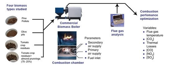
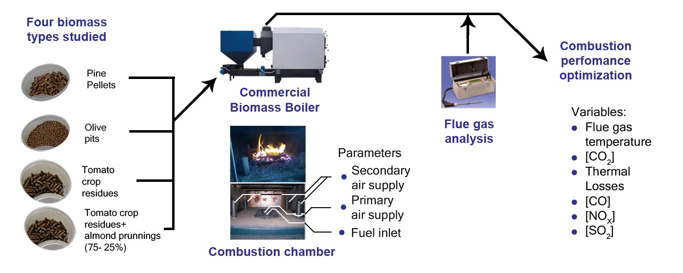
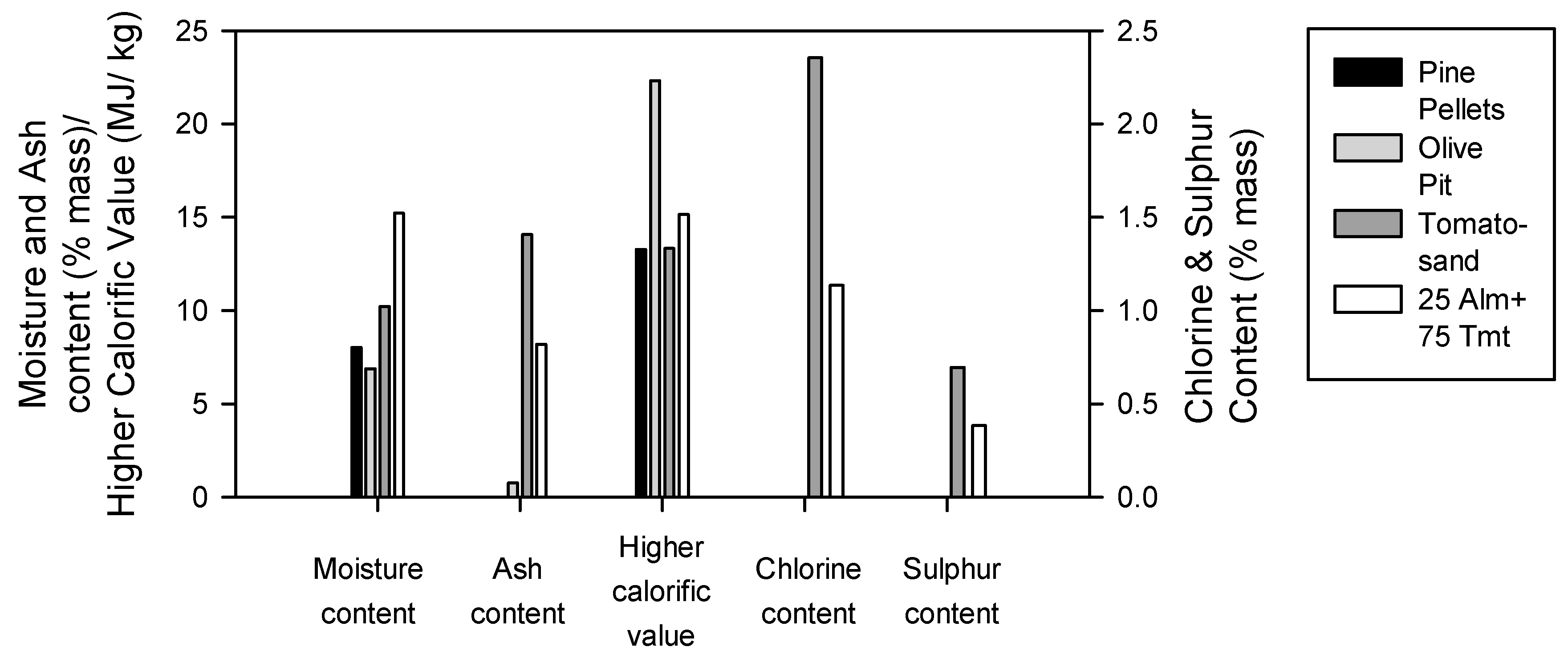
2.1. Biomass
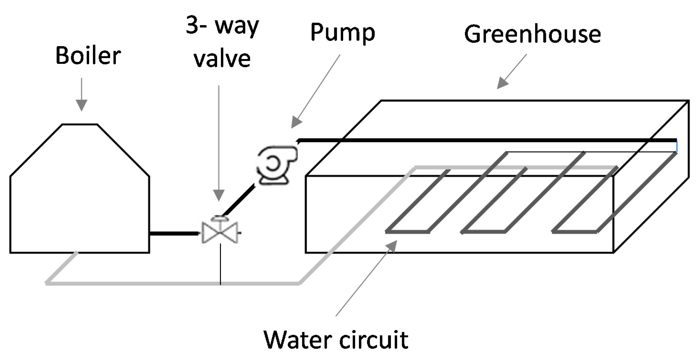
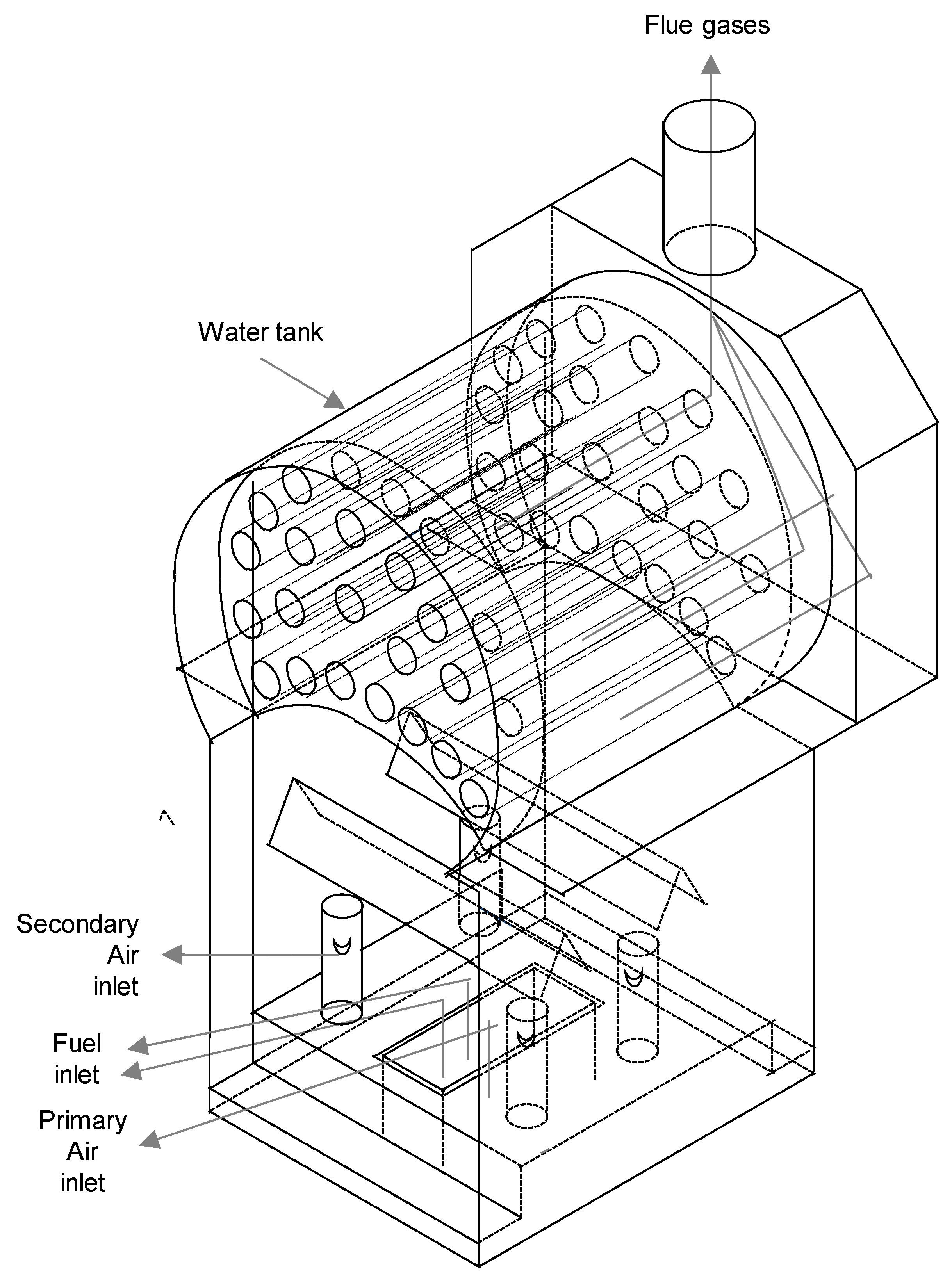
2.2. Boiler
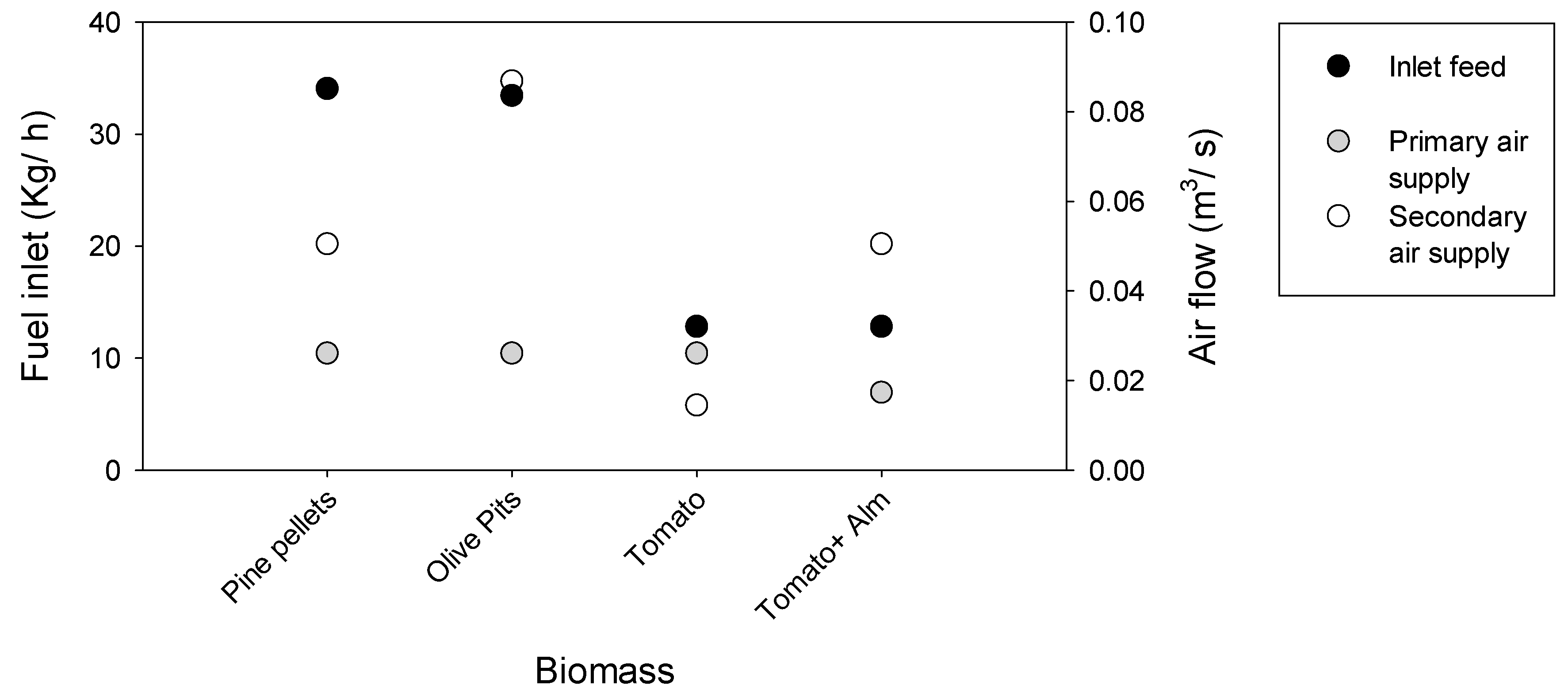
2.3. Combustion Optimization Assays
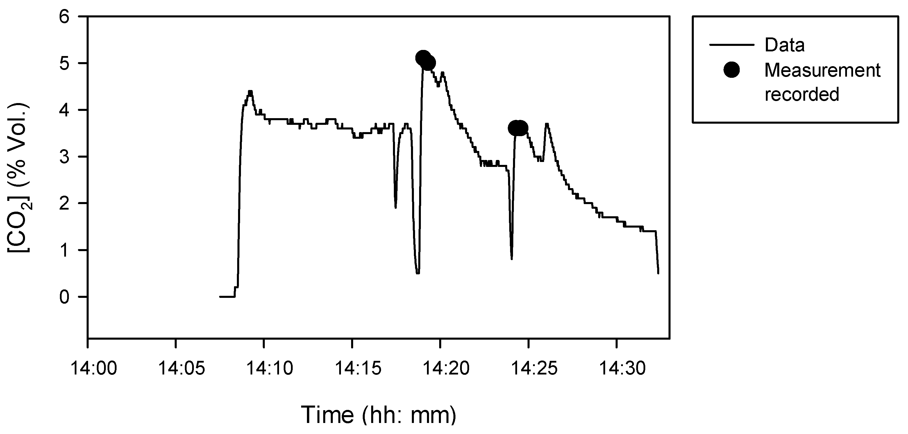
2.4. Flue-Gas Temperature and CO2
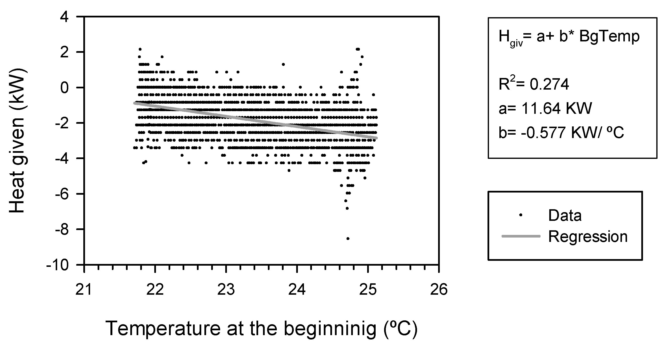
2.5. Thermal and Heating Efficiency Measurements
2.6. CO, NOX, and SO2 Flue-Gas Measurements
2.7. Posterior Reduction in CO, NOX, and SO2 Emissions during CO2 Capture
2.8. Statistical Analysis.
2.9. Particle Emissions
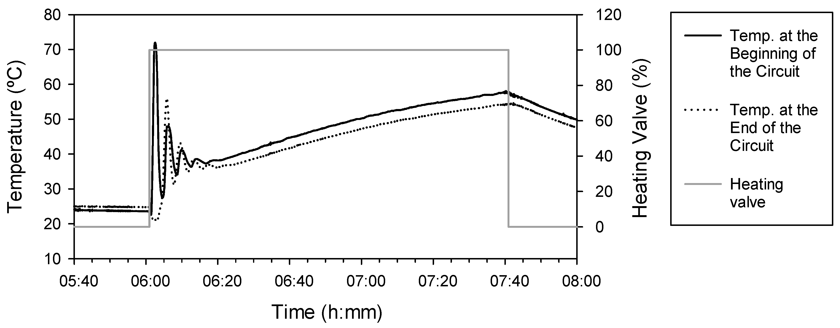
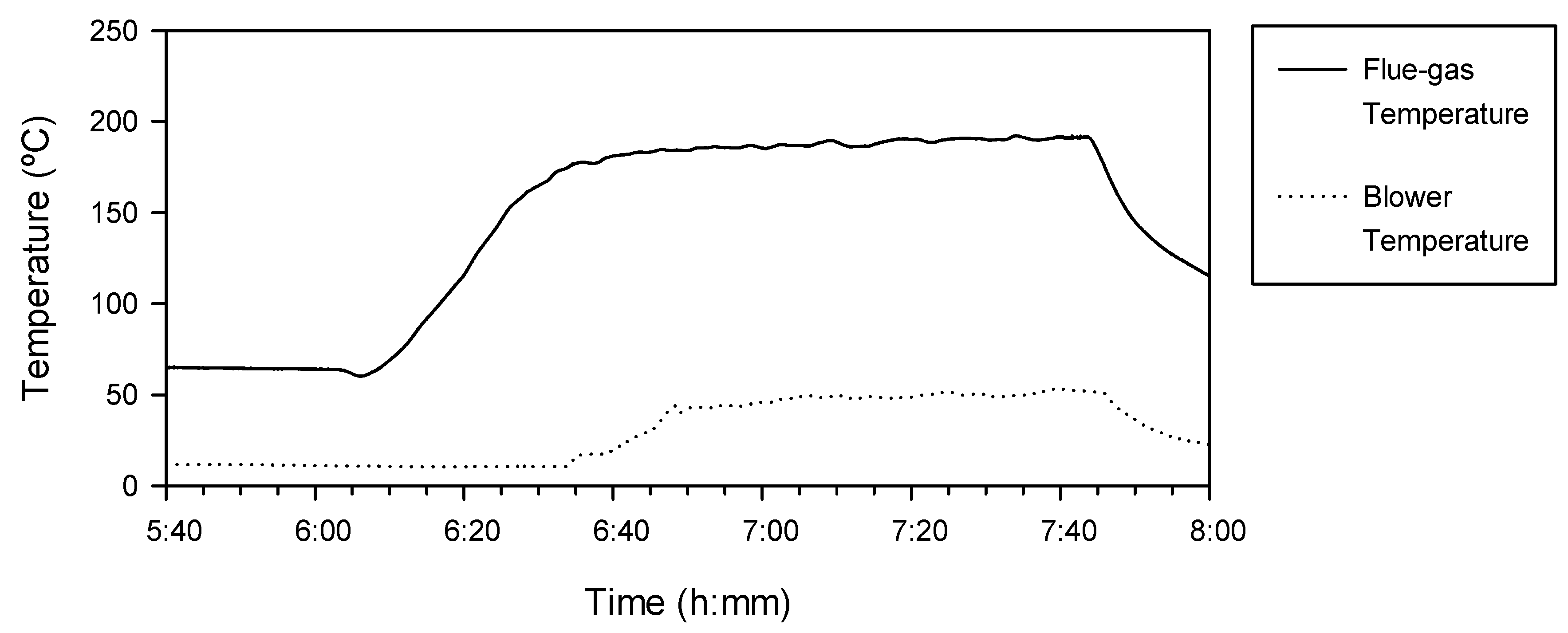
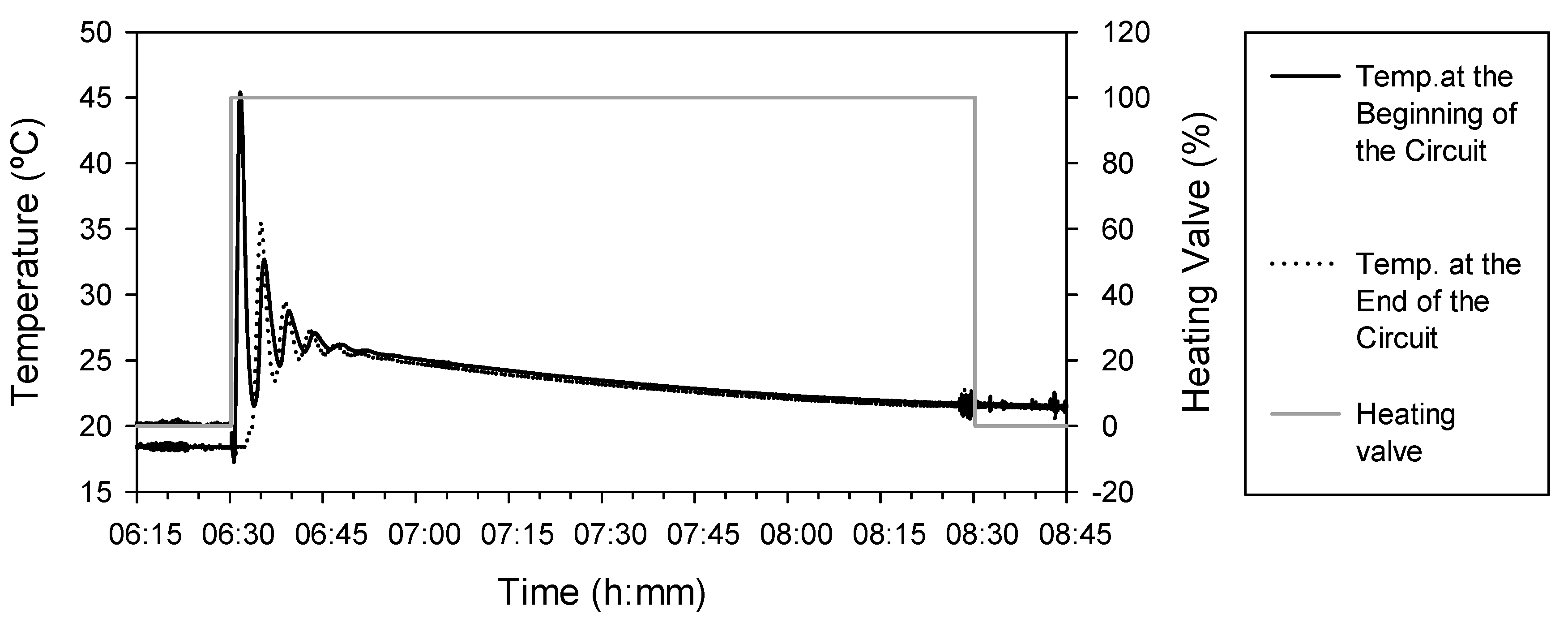
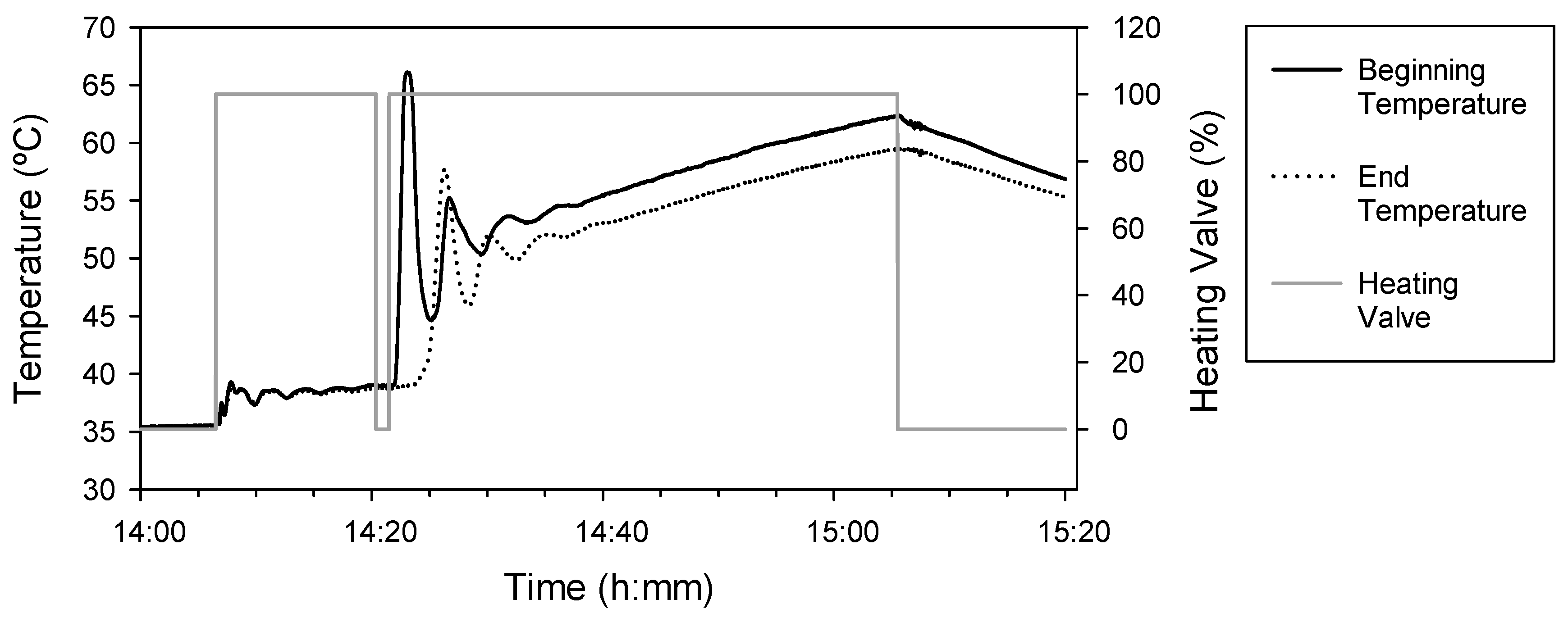
2.10. Heating and Enrichment Experiments over Long Periods
3. Results
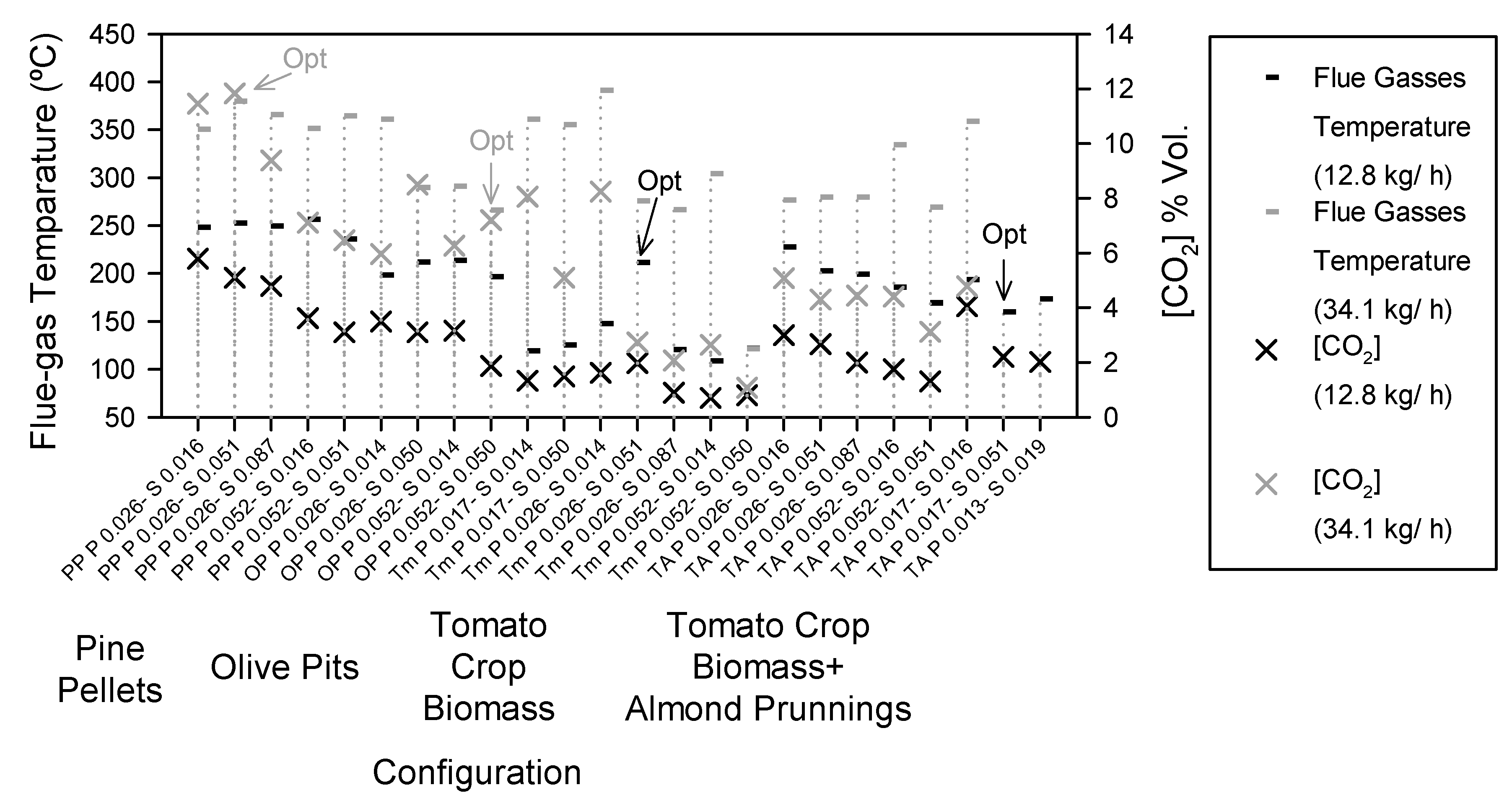
3.1. Flue-Gas Temperature and [CO2]
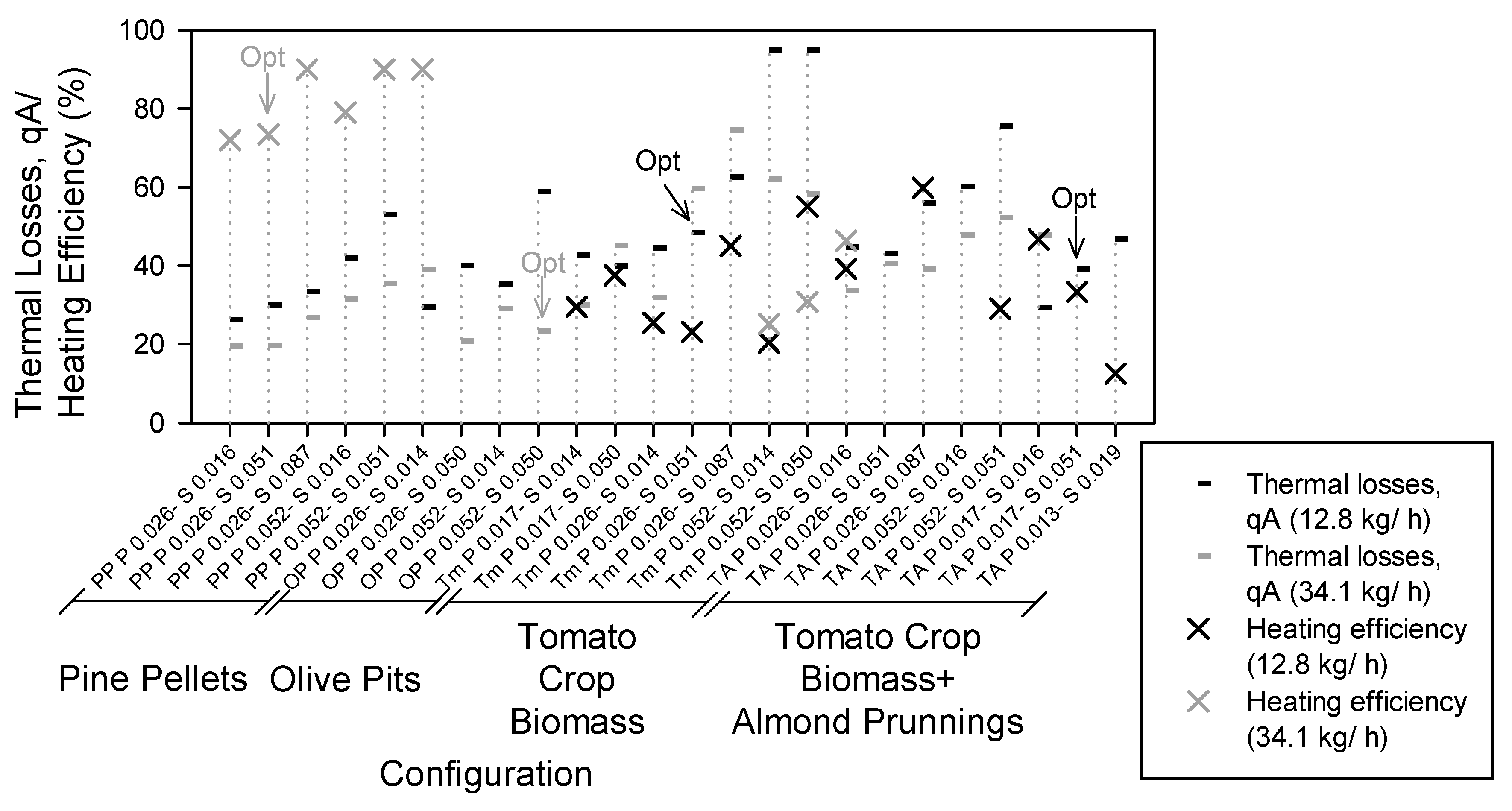
3.2. Thermal and Heating Efficiency
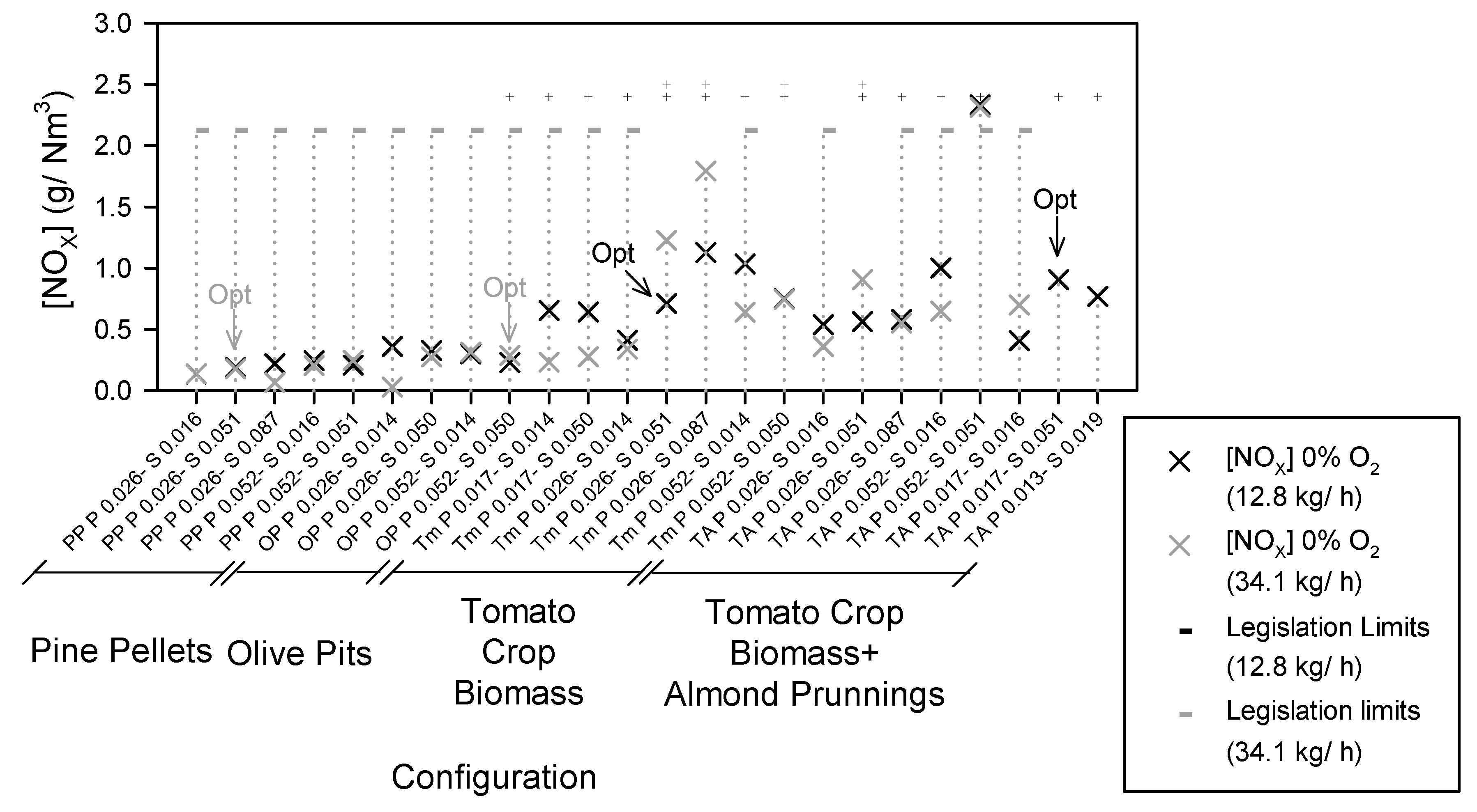
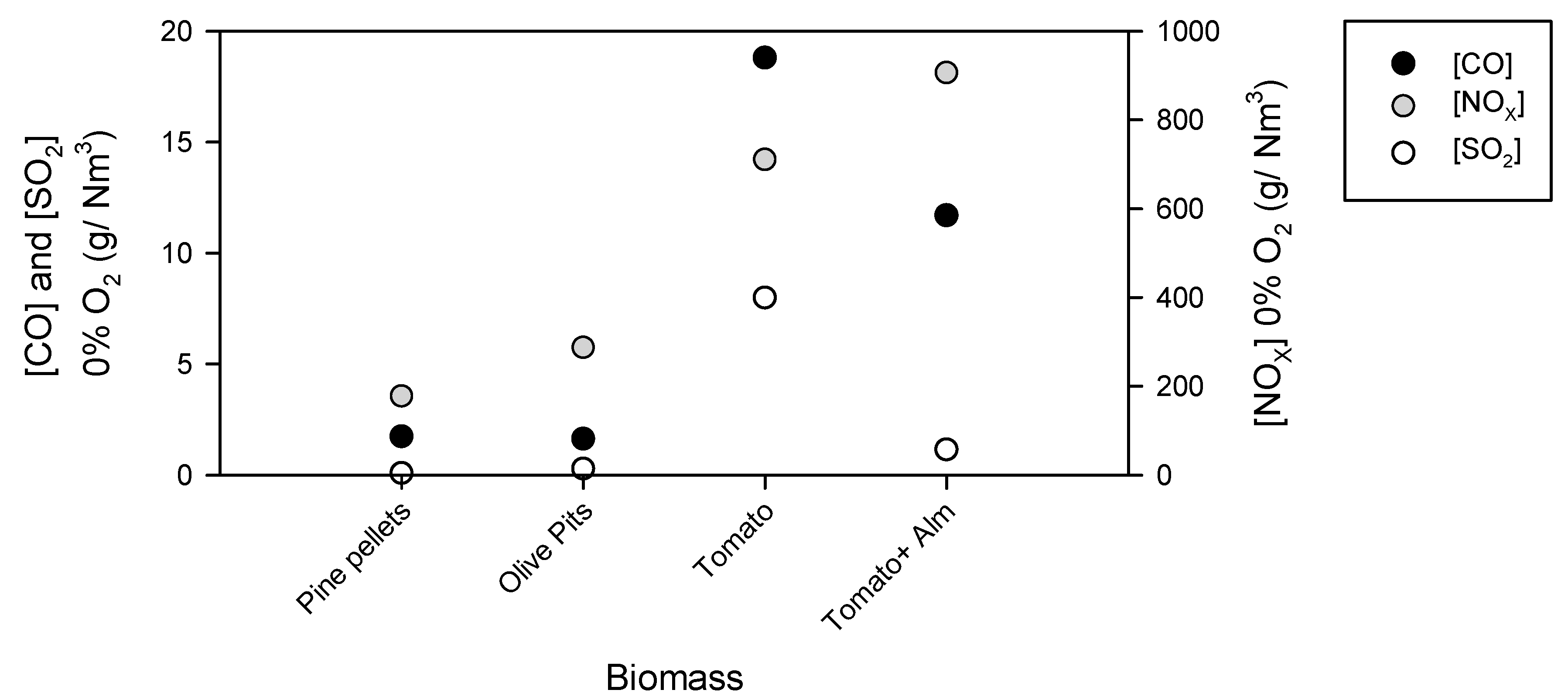
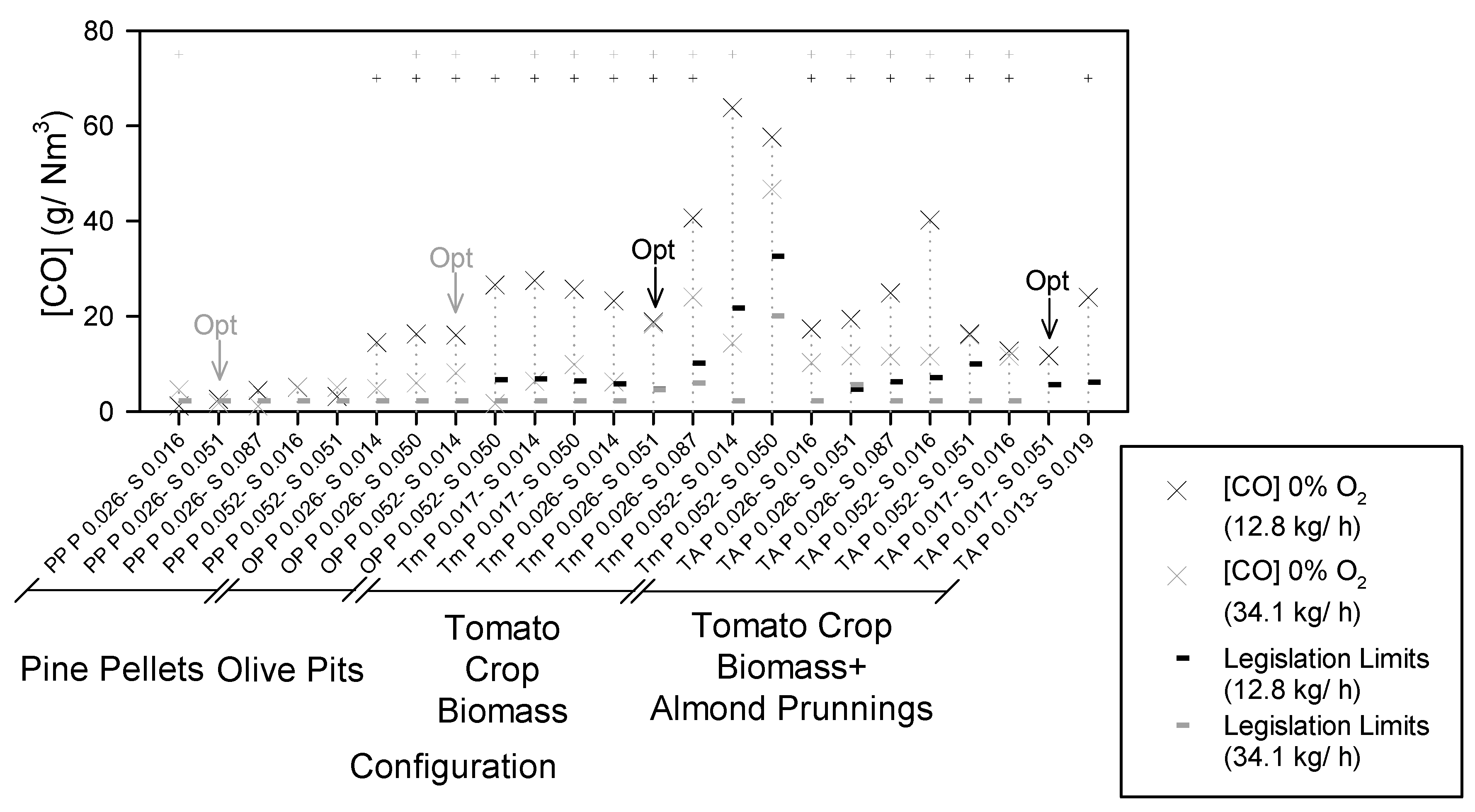
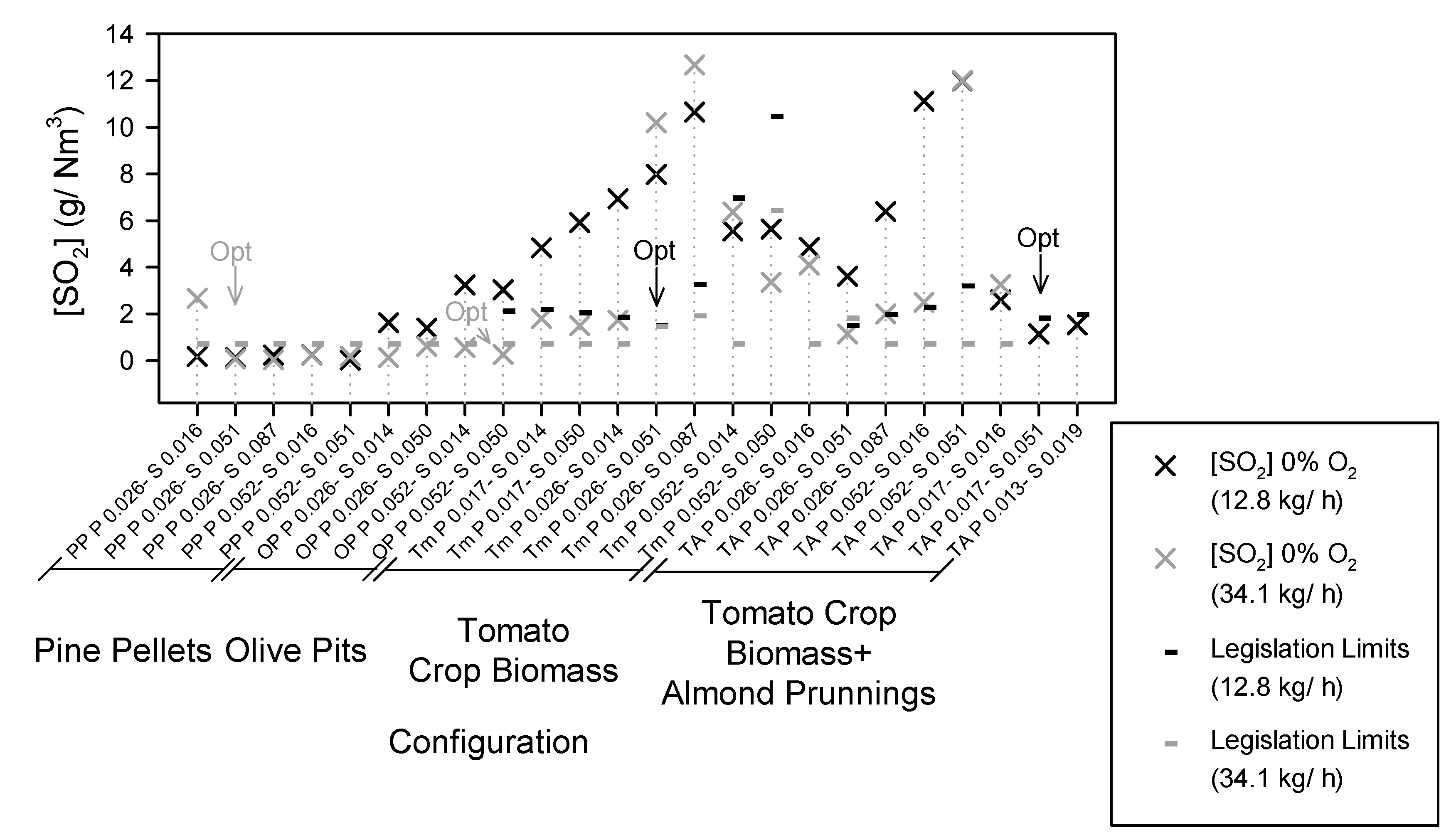
3.3. [CO], NOX, and SO2 in the Flue Gasses
3.4. Posterior Reductions in CO, NOX, and SO2 Emissions during CO2 Capture
3.5. Particle Emissions
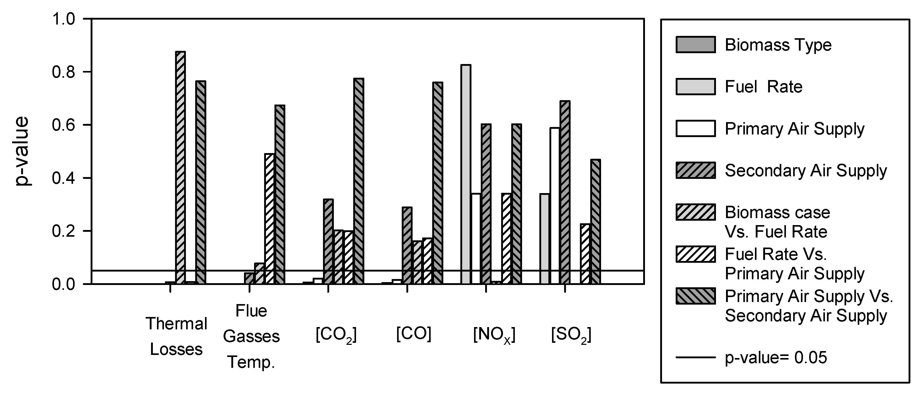
3.6. Statistical Analysis
3.7. Heating and Enrichment Experiments over the Long Term
4. Discussion
5. Conclusions
6. Patents
Author Contributions
Funding
Institutional Review Board Statement
Informed Consent Statement
Data Availability Statement
Acknowledgments
Conflicts of Interest
Appendix A. Methodology, Additional Considerations
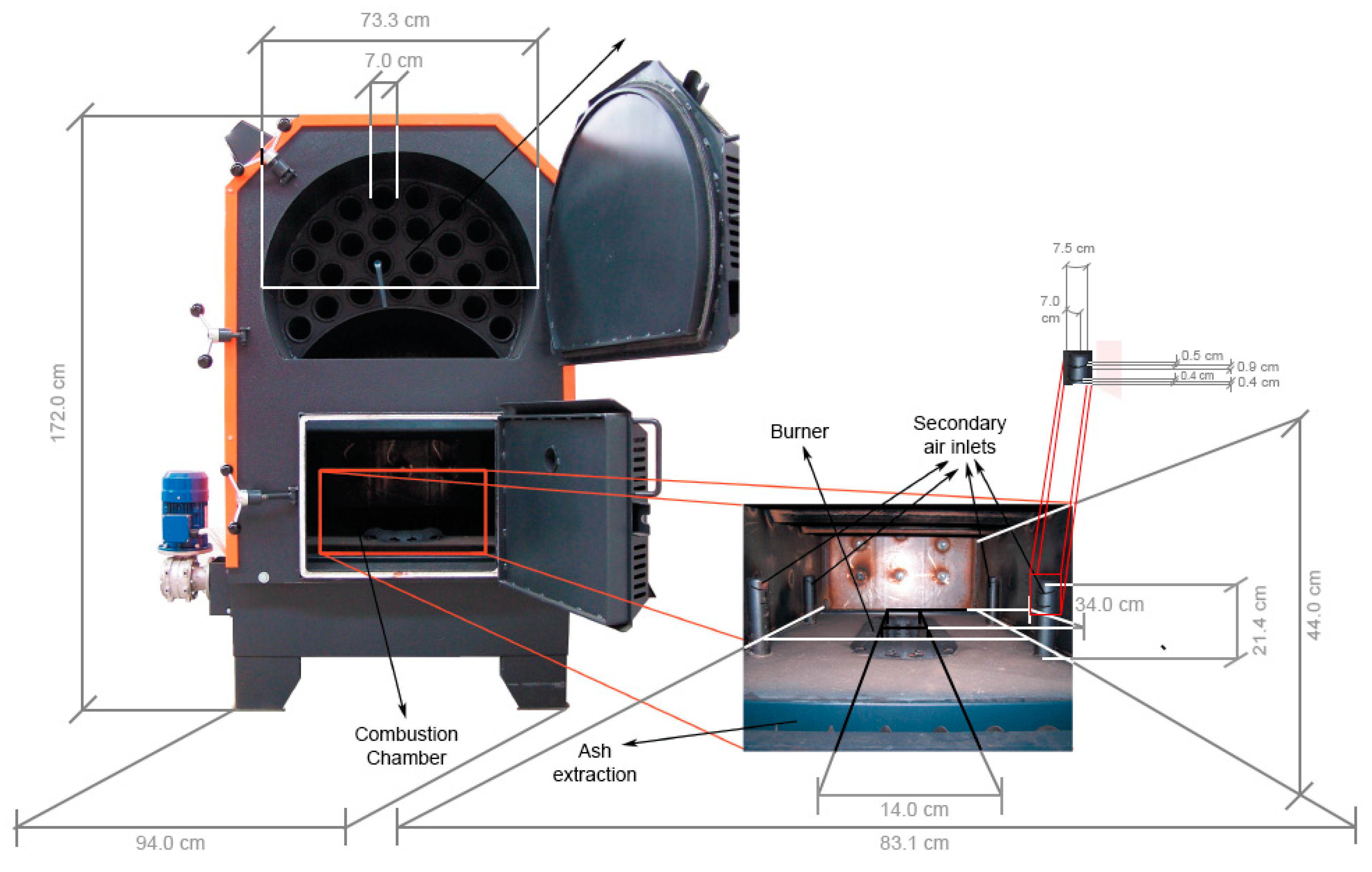
Appendix A.1. Boiler Internal Design

Appendix A.2. Methods Applied for the Flue-Gas Measurements (Thermal Efficiency, CO2, CO, NOX, and SO2)

Appendix B. Heating Efficiency Estimation
Appendix B.1. Discontinuous Experiments


Appendix B.2. Estimation of the Combustion Efficiency at Any Moment


Appendix C. Results and Discussion—Additional Considerations
Appendix C.1. Flue-Gas Temperature and [CO2]
Appendix C.2. Thermal and Heating Efficiency
Appendix C.3. [CO], [NOX], and [SO2] in the Flue Gases
Appendix C.4. Statistical Analysis

| Parameter | Source | Sum of Squares | Df | Mean Square | F-Ratio | P-Value |
|---|---|---|---|---|---|---|
| Flue-gas temperature | MAIN EFFECTS | |||||
| A: Biomass type | 4324.19 | 3 | 1441.4 | 17.73 | 0.0000 | |
| B: Fuel rate | 796.175 | 1 | 796.175 | 9.79 | 0.0053 | |
| C: Primary air supply | 516.884 | 1 | 516.884 | 6.36 | 0.0203 | |
| RESIDUAL | 1626.22 | 20 | 81.3111 | |||
| TOTAL (CORRECTED) | 7910.74 | 31 | ||||
| Thermal efficiency | MAIN EFFECTS | |||||
| A: Biomass type | 6796.97 | 3 | 2265.66 | 41.48 | 0.0000 | |
| B: Fuel rate | 1006.88 | 1 | 1006.88 | 18.43 | 0.0004 | |
| C: Primary air supply | 2040.01 | 1 | 2040.01 | 37.35 | 0.0000 | |
| D: Secondary air supply | 500.07 | 1 | 500.07 | 9.16 | 0.0067 | |
| INTERACTIONS | ||||||
| BC | 487.5 | 1 | 487.5 | 8.92 | 0.0073 | |
| RESIDUAL | 1092.45 | 20 | 54.6224 | |||
| TOTAL (CORRECTED) | 11,966.3 | 31 | ||||
| [CO2] | MAIN EFFECTS | |||||
| A: Biomass type | 120.535 | 3 | 40.1783 | 29.95 | 0.0000 | |
| B: Fuel rate | 71.4013 | 1 | 71.4013 | 53.22 | 0.0000 | |
| C: Primary air supply | 18.0 | 1 | 18.0 | 13.42 | 0.0015 | |
| D: Secondary air supply | 6.48 | 1 | 6.48 | 4.83 | 0.0399 | |
| RESIDUAL | 26.8325 | 20 | 1.34163 | |||
| TOTAL (CORRECTED) | 254.82 | 31 | ||||
| [CO] | MAIN EFFECTS | |||||
| A: Biomass type | 4324.19 | 3 | 1441.4 | 20.41 | 0.0000 | |
| B: Fuel rate | 796.175 | 1 | 796.175 | 11.27 | 0.0037 | |
| C: Primary air supply | 516.884 | 1 | 516.884 | 7.32 | 0.0150 | |
| RESIDUAL | 1200.87 | 17 | 70.6393 | |||
| TOTAL (CORRECTED) | 7910.74 | 31 | ||||
| [NOX] | MAIN EFFECTS | |||||
| A: Biomass type | 5.05303 | 3 | 1.68434 | 12.38 | 0.0002 | |
| D: Secondary air supply | 0.618828 | 1 | 0.618828 | 4.55 | 0.0478 | |
| INTERACTIONS | ||||||
| AC | 2.20263 | 3 | 0.73421 | 5.40 | 0.0085 | |
| RESIDUAL | 2.31231 | 17 | 0.136018 | |||
| TOTAL (CORRECTED) | 10.588 | 31 | ||||
| [SO2] | MAIN EFFECTS | |||||
| A: Biomass type | 304.908 | 3 | 101.636 | 24.59 | 0.0000 | |
| INTERACTIONS | ||||||
| AC | 127.58 | 3 | 42.5268 | 10.29 | 0.0003 | |
| RESIDUAL | 82.6784 | 20 | 4.13392 | |||
| TOTAL (CORRECTED) | 529.772 | 31 |
Appendix C.5. Optimal Configurations


Appendix D. Graphical Comparison with the Bibliography Results
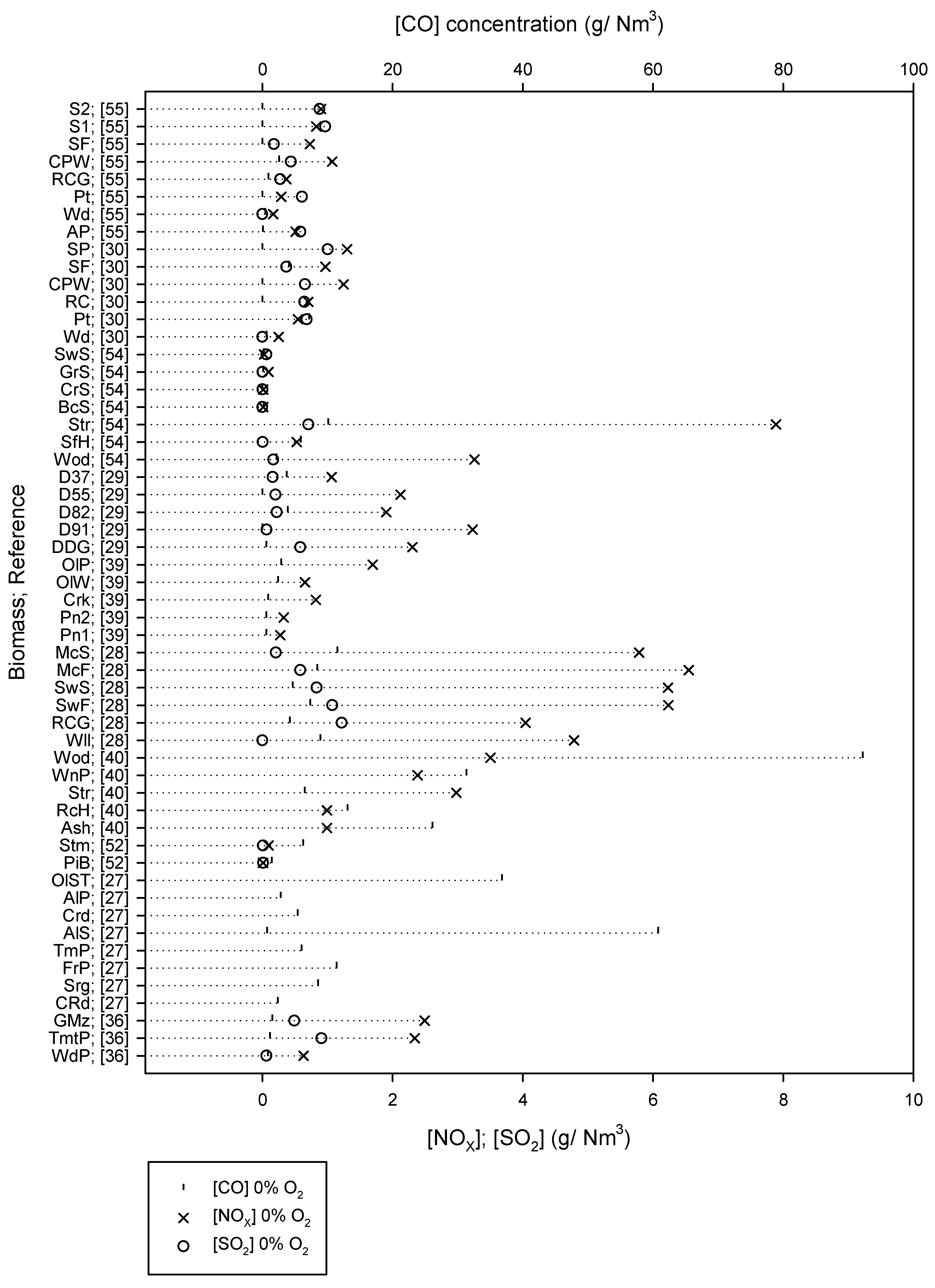
| Reference | Biomass | Abbreviation |
|---|---|---|
| [36] | Wood pellets | WdP; [36] |
| Tomato pomace | TmtP; [36] | |
| Grape maize | GMz; [36] | |
| [27] | Common reed | CRd; [27] |
| Sorghum Sorghum | Srg; [27] | |
| Forest pellets | FrP; [27] | |
| Tomato pomace | TmP; [27] | |
| Almond shells | AlS; [27] | |
| Cardoon | Crd; [27] | |
| Almond prunings | AlP; [27] | |
| Almond shell peel | AlS; [27] | |
| Olive stones | OlST; [27] | |
| [52] | Pine bark | PiB; [52] |
| Stem wood | Stm; [52] | |
| [40] | Almond shells | Ash; [40] |
| Rice husks | RcH; [40] | |
| Straw | Str; [40] | |
| Wine pomace | WnP; [40] | |
| Wood pellets | Wod; [40] | |
| [28] | Willow | Wll; [28] |
| Red canary grass | RCG; [28] | |
| Switchgrass (Fall) | SwF; [28] | |
| Switchgrass (Spring) | SwS; [28] | |
| Miscanthus (Fall) | McF; [28] | |
| Miscanthus (Spring) | McS; [28] | |
| [39] | Pine (1) | Pn1; [39] |
| Pine (2) | Pn2; [39] | |
| Cork | Crk; [39] | |
| Olive wood | OlW; [39] | |
| Olive prunings | OlP; [39] | |
| [53] | Poplar woodchips | PpW; [53] |
| [29] | Dried distilled grain | DDG; [29] |
| Dried distilled grain + Municipal waste solids (90–10%) | D91; [29] | |
| Dried distilled grain + Municipal waste solids (80–20%) | D82; [29] | |
| Dried distilled grain + Municipal waste solids (50–50%) | D55; [29] | |
| Dried distilled grain + Municipal waste solids (30–70%) | D37; [29] | |
| [54] | Wood | Wod; [54] |
| Sunflower stalks | SfH; [54] | |
| Straw | Str; [54] | |
| Buckwheat shells | BcS; [54] | |
| Cornstalk | CrS; [54] | |
| Grain screenings | GrS; [54] | |
| Sewage sludge | SwS; [54] | |
| [30] | Wood | Wd; [30] |
| Peat | Pt; [30] | |
| Reed canary grass | RC; [30] | |
| Citrus pectin waste | CPW; [30] | |
| Sunflower husk | SF; [30] | |
| Straw pellets | SP; [30] | |
| Apple pomace waste | AP; [55] | |
| [55] | Wood | Wd; [55] |
| Peat | Pt; [55] | |
| Reed canary grass | RCG; [55] | |
| Citrus pectin waste | CPW; [55] | |
| Sunflower husks | SF; [55] | |
| Straw pellets 1 | S1; [55] | |
| Straw pellets 2 | S2; [55] |
| Reference | Equipment | Thermal Output (KW) | Biomass | [CO] 0% O2 (mg/Nm3) | [NOX] 0% O2 (mg/Nm3) | [SO2] 0% O2 (mg/Nm3) | Efficiency (%) |
|---|---|---|---|---|---|---|---|
| [36] | Pellet boiler | 12.0 | Wood pellets | 829.3 | 633.9 | 62.9 | |
| Tomato pomace | 1186.4 | 2338.9 | 908.0 | ||||
| Grape maize | 1512.4 | 2491.9 | 491.3 | ||||
| [27] | Pellet boiler | 12.0 | Common reed | 2358.9 | 84.0 | ||
| Sorghum | 8562.3 | 85.3 | |||||
| Forest pellets | 11,398.9 | 90.5 | |||||
| Tomato pomace | 6006.3 | 91.0 | |||||
| Almond shells | 712.5 | 85.0 | |||||
| Cardoon | 5404.0 | 91.6 | |||||
| Almond prunings | 2804.9 | 88.3 | |||||
| Almond shell peel | 60,755.8 | 78.5 | |||||
| Olive stones | 36,798.0 | 89.7 | |||||
| [52] | Small combustion device | 50.0 | Pine bark | 1476.9 | 8.6 | 12.3 | |
| Stem wood | 6252.4 | 93.1 | 9.6 | ||||
| [40] | Tubular furnace (Lab. Scale) | Almond shells | 26,125.0 | 992.8 | |||
| Rice husks | 13,062.5 | 992.8 | |||||
| Straw | 6531.3 | 2978.3 | |||||
| Wine pomace | 31,350.0 | 2382.6 | |||||
| Wood pellets | 92,205.9 | 3503.8 | |||||
| [28] | Biomass boiler | 29.0 | Willow | 8917.1 | 4786.4 | ||
| Red canary grass | 4246.4 | 4042.1 | 1218.0 | ||||
| Switchgrass (Fall) | 7336.3 | 6235.1 | 1073.6 | ||||
| Switchgrass (Spring) | 4641.4 | 6228.3 | 832.0 | ||||
| Miscanthus (Fall) | 8459.4 | 6549.1 | 583.3 | ||||
| Miscanthus (Spring) | 11,496.8 | 5785.4 | 206.1 | ||||
| [39] | Pellet-fired boiler | 22.0 | Pine (1) | ||||
| Pine (2) | 599.2 | 273.2 | |||||
| Cork | 623.2 | 327.9 | |||||
| Olive wood | 886.8 | 819.7 | |||||
| Olive prunings | 2396.8 | 655.8 | |||||
| [53] | Fired-bed boiler | 140.0 | Poplar woodchips | 2876.1 | 1694.1 | 94.0 | |
| [29] | Fluidized bed combustor; 6 Kg/h | Dried distilled grain | |||||
| Dried distilled grain + Municipal waste solids (90–10%) | 592.5 | 2302.8 | 583.4 | ||||
| Dried distilled grain + Municipal waste solids (80–20%) | 3228.0 | 64.0 | |||||
| Dried distilled grain + Municipal waste solids (50–50%) | 3891.0 | 1901.0 | 221.8 | ||||
| Dried distilled grain + Municipal waste solids (30–70%) | 2120.1 | 201.9 | |||||
| [54] | Pellet boiler | 35.0 | Wood | 3732.1 | 1063.7 | 159.5 | |
| Sunflower stalks | 2178.8 | 3257.2 | 167.1 | ||||
| Straw | 5925.4 | 526.6 | 3.6 | ||||
| Buckwheat shells | 10,099.6 | 7886.3 | 707.9 | ||||
| Corn stalk | 196.8 | 12.3 | 0.0 | ||||
| Grain screenings | 16.5 | 10.6 | 1.9 | ||||
| Sewage sludge | 141.0 | 93.8 | 1.8 | ||||
| [30] | Multi-fuel boiler, Reduced Load | 40.0 | Wood | 263.3 | 27.1 | 62.2 | 93.0 |
| Peat | 36,376.6 | 527.8 | 143.3 | 94.1 | |||
| Reed canary grass | 91.7 | ||||||
| Citrus pectin waste | 658.1 | 250.1 | 89.9 | ||||
| Sunflower husks | 89.1 | ||||||
| Straw pellets | 7195.1 | 546.8 | 681.7 | 89.8 | |||
| Apple pomace waste | 704.2 | 644.7 | 91.0 | ||||
| [55] | Multi-fuel boiler, Reduced Load | 40.0 | Wood | 1247.1 | 654.3 | ||
| Peat | 4114.2 | 967.3 | 368.7 | 90.0 | |||
| Reed canary grass | 1299.1 | 1002.9 | 89.8 | ||||
| Citrus pectin waste | 81.0 | 509.9 | 584.4 | 89.7 | |||
| Sunflower husks | 424.2 | 166.8 | 0.0 | 89.0 | |||
| Straw pellets 1 | 289.4 | 609.4 | 88.9 | ||||
| Straw pellets 2 | 903.6 | 367.2 | 274.2 | 88.0 |
References
- Mazuela, P.; Urrestarazu, M.; Bastias, E. Vegetable Waste Compost Used as Substrate in Soilless Culture. Crop Prod. Technol. 2012. [Google Scholar] [CrossRef] [Green Version]
- Haque, A.; Mondal, D.; Khan, I.; Usmani, M.A.; Bhat, A.H.; Gazal, U. Fabrication of composites reinforced with lignocellulosic materials from agricultural biomass. In Lignocellulosic Fibre and Biomass-Based Composite Materials; Elsevier: Amsterdam, The Netherlands, 2017; pp. 179–191. [Google Scholar]
- Kalderis DKoutoulakis DParaskeva PDiamadopoulos EOtal E del Valle, J.O.; Fernández-Pereira, C. Adsorption of polluting substances on activated carbons prepared from rice husk and sugarcane bagasse. Chem. Eng. J. 2008, 144, 42–50. [Google Scholar]
- Pinna-Hernández, M.G.; Martínez-Soler, I.; Villanueva, M.J.D.; Fernández, F.G.A.; López, J.L.C. Selection of biomass supply for a gasification process in a solar thermal hybrid plant for the production of electricity. Ind. Crops Prod. 2019, 137, 339–346. [Google Scholar] [CrossRef]
- Salem, H.B.; Smith, T. Feeding strategies to increase small ruminant production in dry environments. Small Rumin. Res. 2008, 77, 174–194. [Google Scholar] [CrossRef]
- Piriou, B.; Vaitilingom, G.; Veyssière, B.; Cuq, B.; Rouau, X. Potential direct use of solid biomass in internal combustion engines. Prog. Energy Combust. Sci. 2013, 39, 169–188. [Google Scholar] [CrossRef]
- Renewable Energy Statistics. 2020. Available online: https://ec.europa.eu/eurostat/statistics-explained/index.php/Renewable_energy_statistics (accessed on 24 March 2021).
- European Parliament and the Council. Directive (EU) on the Promotion of the Use of Energy from Renewable Sources; Official Journal of the European Union. L 328/82; European Union: Brussels, Belgium, 2017. Available online: https://eur-lex.europa.eu/legal-content/EN/TXT/HTML/?uri=CELEX:32018L2001&from=EN (accessed on 24 March 2021).
- Cajamar Caja Rural Agro-Food Studies Service. Crop Year Analysis in Almería. 2018. Available online: https://infogram.com/analisis-de-la-campana-hortofruticola-1hd12y9wyv3x6km (accessed on 24 March 2021).
- Gervás, G.E.; Losa, S.M.; Pérez, J.J.L. Yearbook of Statistics Forecast of 2018; Ministry of Agriculture, Fishing and Food Supply of Spain, 2019; Available online: https://www.mapa.gob.es/en/estadistica/temas/publicaciones/anuario-de-estadistica/2019/default.aspx (accessed on 24 March 2021).
- Aznar-Sánchez, J.A.; Velasco-Muñoz, J.F.; García-Arca, D.; López-Felices, B. Identification of Opportunities for Applying the Circular Economy to Intensive Agriculture in Almería (South-East Spain). Agronomy 2020, 10, 1499. [Google Scholar] [CrossRef]
- Reicosky, D.C.; Wilts, A.R. Crop-Residue Management. In Encyclopedia of Soils in the Environment; Elsevier: Amsterdam, The Netherlands, 2005; pp. 334–338. [Google Scholar]
- Duque-Acevedo, M.; Belmonte-Ureña, L.J.; Toresano-Sánchez, F.; Camacho-Ferre, F. Biodegradable Raffia as a Sustainable and Cost-Effective Alternative to Improve the Management of Agricultural Waste Biomass. Agronomy 2020, 10, 1261. [Google Scholar] [CrossRef]
- Callejón-Ferre, A.J.; Velázquez-Martí, B.; López-Martínez, J.A.; Manzano-Agugliaro, F. Greenhouse crop residues: Energy potential and models for the prediction of their higher heating value. Renew. Sustain. Energy Rev. 2011, 15, 948–955. [Google Scholar] [CrossRef]
- Moreno, J.R.; Pinna-Hernández, G.; Fernández, M.F.; Molina, J.S.; Díaz, F.R.; Hernández, J.L.; Fernández, F.A. Optimal processing of greenhouse crop residues to use as energy and CO2 sources. Ind. Crops Prod. 2019, 137, 662–671. [Google Scholar] [CrossRef]
- Djunisic, S. Spain’s Ence working on 330 MW of biomass, solar projects in Andalusia. Renew. Now 2020. Available online: https://worldwide.espacenet.com/patent/search/family/051752201/publication/ES2514090A1?q=pn%3DES2514090A1 (accessed on 24 March 2021).
- Acién, F.G.; Fernández-Sevilla, J.M.; Grima, E.M. Supply of CO2 to closed and open photobioreactors. In Microalgal Production for Biomass and High-Value Products; Slocombe, S., Benemann, J., Eds.; CRC Press: Boca Raton, FL, USA, 2016; pp. 225–252. [Google Scholar]
- Assunção, J.; Batista, A.P.; Manoel, J.; da Silva, T.L.; Marques, P.; Reis, A.; Gouveia, L. CO2 utilization in the production of biomass and biocompounds by three different microalgae. Eng. Life Sci. 2017, 17, 1126–1135. [Google Scholar] [CrossRef] [Green Version]
- Assunção, J.; Malcata, F.X. Enclosed ‘non-conventional’ photobioreactors for microalga production: A review. Algal Res. 2020, 52, 102107. [Google Scholar] [CrossRef]
- Dion, L.-M.; Lefsrud, M.; Orsat, V. Review of CO2 recovery methods from the exhaust gas of biomass heating systems for safe enrichment in greenhouses. Biomass Bioenergy 2011, 35, 3422–3432. [Google Scholar] [CrossRef]
- Roy, Y.; Lefsrud, M.; Orsat, V.; Filion, F.; Bouchard, J.; Nguyen, Q.; Dion, L.M.; Glover, A.; Madadian, E.; Lee, C.P. Biomass combustion for greenhouse carbon dioxide enrichment. Biomass Bioenergy 2014, 66, 186–196. [Google Scholar] [CrossRef]
- Hukkanen, A.; Kaivosoja, T.; Sippula, O.; Nuutinen, K.; Jokiniemi, J.; Tissari, J. Reduction of gaseous and particulate emissions from small-scale wood combustion with a catalytic combustor. Atmos. Environ. 2012, 50, 16–23. [Google Scholar] [CrossRef]
- Kraszkiewicz, A.; Przywara, A.; Anifantis, A.S. Impact of Ignition Technique on Pollutants Emission during the Combustion of Selected Solid Biofuels. Energies 2020, 13, 2664. [Google Scholar] [CrossRef]
- Carvalho, L.; Wopienka, E.; Pointner, C.; Lundgren, J.; Verma, V.K.; Haslinger, W.; Schmidl, C. Performance of a pellet boiler fired with agricultural fuels. Appl. Energy 2013, 104, 286–296. [Google Scholar] [CrossRef]
- Mortensen, L.M. Nitrogen oxides produced during CO2 enrichment. I. Effects on different greenhouse plants. New Phytol. 1985, 101, 103–108. [Google Scholar] [CrossRef]
- Caporn, S.J.M. The effects of oxides of nitrogen and carbon dioxide enrichment on photosynthesis and growth of lettuce (Lactuca sativa L.). New Phytol. 1989, 111, 473–481. [Google Scholar] [CrossRef]
- González, J.F.; González-García, C.M.; Ramiro, A.; Gañán, J.; Ayuso, A.; Turegano, J. Use of energy crops for domestic heating with a mural boiler. Fuel Process. Technol. 2006, 87, 717–726. [Google Scholar] [CrossRef]
- Fournel, S.; Marcos, B.; Godbout, S.; Heitz, M. Predicting gaseous emissions from small-scale combustion of agricultural biomass fuels. Bioresour. Technol. 2015, 179, 165–172. [Google Scholar] [CrossRef] [PubMed]
- Laryea-Goldsmith, R.; Oakey, J.; Simms, N.J. Gaseous emissions during concurrent combustion of biomass and non-recyclable municipal solid waste. Chem. Cent. J. 2011, 5, 4. [Google Scholar] [CrossRef] [Green Version]
- Verma, V.K.; Bram, S.; Gauthier, G.; de Ruyck, J. Performance of a domestic pellet boiler as a function of operational loads: Part-2. Biomass Bioenergy 2011, 35, 272–279. [Google Scholar] [CrossRef]
- Callejón-Ferre, A.J.; Carreño-Sánchez, J.; Suárez-Medina, F.J.; Pérez-Alonso, J.; Velázquez-Martí, B. Prediction models for higher heating value based on the structural analysis of the biomass of plant remains from the greenhouses of Almería (Spain). Fuel 2014, 116, 377–387. [Google Scholar] [CrossRef]
- Morales, L.; Garzón, E.; Martínez-Blanes, J.M.; Sánchez-Soto, P.J. Thermal study of residues from greenhouse crops plant biomass. J. Therm. Anal. Calorim. 2017, 129, 1111–1120. [Google Scholar] [CrossRef]
- Sánchez-Molina, J.A.; Reinoso, J.V.; Acién, F.G.; Rodríguez, F.; López, J.C. Development of a biomass-based system for nocturnal temperature and diurnal CO2 concentration control in greenhouses. Biomass Bioenergy 2014, 67, 60–71. [Google Scholar] [CrossRef]
- Pinna-Hernández, M.G.; Fernández, F.G.A.; Segura, J.G.L.; López, J.L.C. Solar Drying of Greenhouse Crop Residues for Energy Valorization: Modeling and Determination of Optimal Conditions. Agronomy 2020, 10, 2001. [Google Scholar] [CrossRef]
- Fernández, F.G.A.; Sevilla, J.M.F.; Hernández, J.C.L.; Díaz, F.R.; Molina, J.A.S. Combined System of Heating and Carbon Enrichment from Biomass. Patent no. ES2514090; European Patent Office, 2014. Available online: https://worldwide.espacenet.com/patent/search/family/051752201/publication/ES2514090A1?q=pn%3DES2514090A1 (accessed on 24 March 2021).
- Kraiem, N.; Lajili, M.; Limousy, L.; Said, R.; Jeguirim, M. Energy recovery from Tunisian agri-food wastes: Evaluation of combustion performance and emissions characteristics of green pellets prepared from tomato residues and grape marc. Energy 2016, 107, 409–418. [Google Scholar] [CrossRef]
- Ito, K. Greenhouse temperature control with wooden pellet heater via model predictive control approach. In Proceedings of the 2012 20th Mediterranean Conference on Control & Automation (MED), Barcelona, Spain, 3–6 July 2012; pp. 1542–1547. [Google Scholar]
- Andalusian Government. Decreto 239/ 2011, 12 de Julio, por el que se Regula la Calidad del Medio Ambiente Atmosférico y se crea el Registro de Sistemas de Evaluación de la Calidad del Aire en Andalucía; BOJA (Boletín Oficial de la Junta de Andalucía): Sevilla, Spain, 4 August 2011. Available online: https://www.juntadeandalucia.es/boja/2011/152/5 (accessed on 24 March 2021).
- Garcia-Maraver, A.; Zamorano, M.; Fernandes, U.; Rabaçal, M.; Costa, M. Relationship between fuel quality and gaseous and particulate matter emissions in a domestic pellet-fired boiler. Fuel 2014, 119, 141–152. [Google Scholar] [CrossRef]
- Fernández, R.G.; García, C.P.; Lavín, A.G.; de las Heras, J.L.B. Study of main combustion characteristics for biomass fuels used in boilers. Fuel Process. Technol. 2012, 103, 16–26. [Google Scholar] [CrossRef]
- Yanik, J.; Duman, G.; Karlström, O.; Brink, A. NO and SO2 emissions from combustion of raw and torrefied biomasses and their blends with lignite. J. Environ. Manag. 2018, 227, 155–161. [Google Scholar] [CrossRef]
- Darvell, L.I.; Brindley, C.; Baxter, X.C.; Jones, J.M.; Williams, A. Nitrogen in Biomass Char and Its Fate during Combustion: A Model Compound Approach. Energy Fuels 2012, 26, 6482–6491. [Google Scholar] [CrossRef]
- Nussbaumer, T. Combustion and Co-combustion of Biomass: Fundamentals, Technologies, and Primary Measures for Emission Reduction †. Energy Fuels 2003, 17, 1510–1521. [Google Scholar] [CrossRef]
- Heschel, W.; Rweyemamu, L.; Scheibner, T.; Meyer, B. Abatement of emissions in small-scale combustors through utilisation of blended pellet fuels. Fuel Process. Technol. 1999, 61, 223–242. [Google Scholar] [CrossRef]
- Wang, L.; Hustad, J.E.; Skreiberg, Ø.; Skjevrak, G.; Grønli, M. A Critical Review on Additives to Reduce Ash Related Operation Problems in Biomass Combustion Applications. Energy Procedia 2012, 20, 20–29. [Google Scholar] [CrossRef] [Green Version]
- Křůmal, K.; Mikuška, P.; Horák, J.; Hopan, F.; Krpec, K. Comparison of emissions of gaseous and particulate pollutants from the combustion of biomass and coal in modern and old-type boilers used for residential heating in the Czech Republic, Central Europe. Chemosphere 2019, 229, 51–59. [Google Scholar] [CrossRef]
- Prochnow, A.; Heiermann, M.; Plöchl, M.; Amon, T.; Hobbs, P.J. Bioenergy from permanent grassland—A review: 2. Combustion. Bioresour. Technol. 2009, 100, 4945–4954. [Google Scholar] [CrossRef]
- Acosta-Motos, J.; Ortuño, M.; Bernal-Vicente, A.; Diaz-Vivancos, P.; Sanchez-Blanco, M.; Hernandez, J. Plant Responses to Salt Stress: Adaptive Mechanisms. Agronomy 2017, 7, 18. [Google Scholar] [CrossRef] [Green Version]
- Gallegos-Cedillo, V.M.; Urrestarazu, M.; Álvaro, J.E. Influence of salinity on transport of nitrates and potassium by means of the xylem sap content between roots and shoots in young tomato plants. J. Soil Sci. Plant Nutr. 2016, 16, 991–998. [Google Scholar] [CrossRef] [Green Version]
- Iáñez-Rodríguez, I.; Martín-Lara, M.Á.; Pérez, A.; Blázquez, G.; Calero, M. Water washing for upgrading fuel properties of greenhouse crop residue from pepper. Renew. Energy 2020, 145, 2121–2129. [Google Scholar] [CrossRef]
- Zhang, N.; Wang, L.; Zhang, K.; Walker, T.; Thy, P.; Jenkins, B.; Zheng, Y. Pretreatment of lignocellulosic biomass using bioleaching to reduce inorganic elements. Fuel 2019, 246, 386–393. [Google Scholar] [CrossRef]
- Dare, P.; Gifford, J.; Hooper, R.J.; Clemens, A.H.; Damiano, L.F.; Gong, D.; Matheson, T.W. Combustion performance of biomass residue and purpose grown species. Biomass Bioenergy 2001, 21, 277–287. [Google Scholar] [CrossRef]
- Caposciutti, G.; Antonelli, M. Experimental investigation on air displacement and air excess effect on CO, CO2 and NO emissions of a small size fixed bed biomass boiler. Renew. Energy 2018, 116, 795–804. [Google Scholar] [CrossRef]
- Krugly, E.; Martuzevicius, D.; Puida, E.; Buinevicius, K.; Stasiulaitiene, I.; Radziuniene, I.; Minikauskas, A.; Kliucininkas, L. Characterization of Gaseous- and Particle-Phase Emissions from the Combustion of Biomass-Residue-Derived Fuels in a Small Residential Boiler. Energy Fuels 2014, 28, 5057–5066. [Google Scholar] [CrossRef]
- Verma, V.K.; Bram, S.; Delattin, F.; Laha, P.; Vandendael, I.; Hubin, A.; De Ruyck, J. Agro-pellets for domestic heating boilers: Standard laboratory and real life performance. Appl. Energy 2012, 90, 17–23. [Google Scholar] [CrossRef]


Publisher’s Note: MDPI stays neutral with regard to jurisdictional claims in published maps and institutional affiliations. |
© 2021 by the authors. Licensee MDPI, Basel, Switzerland. This article is an open access article distributed under the terms and conditions of the Creative Commons Attribution (CC BY) license (http://creativecommons.org/licenses/by/4.0/).
Share and Cite
Reinoso Moreno, J.V.; Pinna Hernández, M.G.; Fernández Fernández, M.D.; Sánchez Molina, J.A.; López Hernández, J.C.; Acién Fernández, F.G. Boiler Combustion Optimization of Vegetal Crop Residues from Greenhouses. Agronomy 2021, 11, 626. https://0-doi-org.brum.beds.ac.uk/10.3390/agronomy11040626
Reinoso Moreno JV, Pinna Hernández MG, Fernández Fernández MD, Sánchez Molina JA, López Hernández JC, Acién Fernández FG. Boiler Combustion Optimization of Vegetal Crop Residues from Greenhouses. Agronomy. 2021; 11(4):626. https://0-doi-org.brum.beds.ac.uk/10.3390/agronomy11040626
Chicago/Turabian StyleReinoso Moreno, José Vicente, María Guadalupe Pinna Hernández, María Dolores Fernández Fernández, Jorge Antonio Sánchez Molina, Juan Carlos López Hernández, and Francisco Gabriel Acién Fernández. 2021. "Boiler Combustion Optimization of Vegetal Crop Residues from Greenhouses" Agronomy 11, no. 4: 626. https://0-doi-org.brum.beds.ac.uk/10.3390/agronomy11040626