Do Erratic Rainfalls Hamper Grain Production? Analysis of Supply Response of Rice to Price and Non-Price Factors

Abstract

Increasing rice production has become one of the ultimate goals for South Asian countries. The yield and area under rice production are also facing threats due to the consequences of climate change such as erratic rainfall and seasonal variation. Thus, the main aim of this work was to find out the supply response of rice in Malaysia in relation to both price and non-price factors. To achieve this target, time series analysis was conducted on data from 1970 to 2014 using cointegration, unit root test, and the vector error correction model. The results showed that the planted area and rainfall have a significant effect on rice production; however, the magnitude of the impact of rainfall is less conspicuous for off-season (season 2) rice as compared to main-season rice (season 1). The speed of adjustment from short-run to long-run for season-1 rice production is almost two-and-a-half years (five production seasons), while for season-2 production, it is only about one-and-a-half year (three production seasons). Consequently, the study findings imply the supply of water to be enhanced through better water infrastructure for both seasons. Moreover, the area under season 2 is continuously declining to the point where the government has to make sure that farmers are able to cultivate the same area for rice production by providing uninterrupted supply of critical inputs, particularly water, seed and fertilizers.

1. Introduction

Rice is considered as an important staple food item of the Malaysian people that plays a key role in the dietary supply among its population. In 2017, the total rice consumption in Malaysia was 2.75 million tons, while the domestic production stood only at about 1.8 million tons, which indicates a self-sufficiency level of about 75 percent in the same period [1]. The gap was substituted with imports from mostly Association of Southeast Asian Nations (ASEAN) countries. The current production of rice is 2.91 million tons, however, the country still imports about 20–24 percent of its rice demand [2,3] with an average consumption of 82 kg per capita per year [4]. Malaysia’s rice venture is too expensive, and the country would need not grow any rice at all if looking from an economic viewpoint such as comparative advantage in relation to the world market. The Malaysian rice supply has been characterized by low quantities, thus limiting the farmers’ incomes. For instance, an alarming level of inefficiency is shown when a relatively low productivity level of 3.9 tons/ha (tons per hectare) for Malaysia is reported in comparison with Indonesia and Vietnam whose productivity stands at 4.9 tons/ha and 5.5 tons/ha, respectively [5].

For small rice-growing countries like Malaysia, the fluctuations in global market conditions create many issues [6]. Major challenges regarding low paddy production in Malaysia are small and uneconomic farm size, aging farmers, high cost of production, and declining natural resource base. Meanwhile, the interest and involvement of the younger generation in paddy planting is decreasing gradually. However, various interventions have been implemented from time to time by the Malaysian government, which included fertilizer subsidies and price support, while import quotas have been imposed to improve the domestic production, farm productivity, farm income, and the achievement of self-sufficiency levels. In this situation, the supply response of Malaysian rice still needs to be addressed despite continuous incentives.

Supply response or supply elasticity is basically developed from supply responses to price changes. Hence, countries like Malaysia need to react more quickly to adjust its domestic prices as their domestic supply is highly dependent on the price of imported rice from neighboring countries. This is necessary in the wake of an increase in global rice prices. However, non-price factors are also very important. Non-price factors, such as environmental conditions (rainfall and sowing season in this study) or planted area, are among the most binding hindrances for the development of agricultural systems [7]. Thus, it is necessary to consider such factors in any serious policy formulations. This helps stabilize price and manage price volatility.

A fundamental question confronting the world is whether price or non-price factors are most important regarding crop supply responses. This study took both price factors and non-price factors such as rainfall and planted area to address this crucial question. Price factors have been considered the main characteristic of profits and supply response of various crops, while supply shifters are exogenous factors such as availability of technology, biophysical conditions such as rainfall that that determine production, and yield risks [8]. For instance, studies have shown that price-supply responses are weak [9], while access to irrigation and rainfall are most important in determining the non-price supply response [10,11]. In the same vein, most crop supply response is dominated by non-price over price factors [12,13]. Farmers may be reluctant to grow more rice because of the imperfect conditions of such factors, e.g., rainfall. For instance, Abraham and Pingali [11] found that yields, rainfall, and irrigation water are significant predictors of area allocation for various crops. Similarly, Kuwornu et al. [13] estimated rice production response in Ghana and found that non-price factors such as rainfall and real price of rice are significant factors.

In this study, two price factors were taken, the price of main-season rice and price of off-season rice. Malaysia is among the unique countries that take two production seasons of rice in a year. Most past studies have tried to address the effect of prices on agricultural supply elasticity at national and household levels in a global perspective framework [14,15,16]. However, empirical research is scanty in terms of checking the effect of price volatility on production. Moreover, most of the authors in recent literature used international prices as a proxy variable for the domestic one [14,15]. This may prevent handling of environmental, social, and political factors that contribute to farmers’ production decisions, particularly at the local level.

Agriculture is the sole source of food, hence, any disturbances to natural resources (due to climate change) may cause severe food shortages as potential changes in climate may reduce output and productivity in agricultural industries. Rice is not an exception, and a changing climate (erratic rainfall patterns in the case of Malaysia) has the potential to impact the yield of rice crop. Despite the costly paddy production in Malaysia, climate change is another threat for paddy production in the country. Therefore, the current study aimed to check the supply response of rice in Malaysia under erratic rainfall conditions. Moreover, the literature shows that overall agricultural productivity in low latitudes is likely to decrease due to climatic variations [17]. Similarly, Chidiebere-Mark et al. [18] conducted an empirical study of rice production under different production systems in developing countries and found that lowland areas have lesser rice productivity compared to uplands. Most developing countries, including Malaysia, are located in lower-latitude regions. Therefore, the best places to increase agricultural yields may be on underperforming landscapes where yields have become marginalized. Hence, the current study is designed to check the supply response of rice in Malaysia and act as a case study for other developing and low-latitude countries.

2. Brief Literature Review on Supply Response

There are a growing number of studies regarding the supply response of agricultural commodities in ASEAN countries except Malaysia. For instance, Guibao [19] found that the rice price elasticities with respect to quantity (production) were in the range of 0.57 to 0.72 in the Philippines. This means that when there is a one unit increase in the price of rice there would be an increase in the production of rice from 57 to 72 percent. Similarly, Erazo-Hinlo and Edgardo [20] found that rice prices are inelastic in the short run as well as in the long run in the Philippines. Inelastic here means farmers are less responsive to change in the prices of rice. Yu and Fan [21] found a rice supply response by applying the Cobb–Douglas production function in Cambodia for dry season paddies and for wet season paddies. They showed that the long-run supply response is bigger and ranges from 1.15 for wet season paddies to 1.45 for dry season paddies with respect to land area, irrigation water, and labor availability. On the other hand, there is a short-run supply elasticity of 0.26 and 0.33 for wet and dry season paddies, respectively. This means that when there is availability of labor, irrigation water, and land area, there would be an increase of 26 to 33 percent in paddy production for dry and wet season rice. Similarly, Edison et al. [22] incorporated price and non-price factors for rice supply response in the Jambi province of Indonesia. They found that elasticity of rice production is 0.1048 in relation to the irrigation index and it has a significant impact on production. This means that there would be a 10.48 percent increase in rice production with the additional availability of irrigation water. Another important study was conducted in Thailand regarding the supply response of rice with respect to the price of biofuel crops [23]. They found supply response is negative in relation to the price of competitive crops (cross price) while it is positive regarding rice price and planted area. They suggested that the government and policy makers should use non-price policies to boost rice production. Thus, our study was designed to fill the gap regarding the supply elasticity of rice in Malaysia, including both price and non-price factors.

The supply response of various crops is dominated by non-price factors over price factors. Non-price factors such as production area, access to irrigation and rainfall [11], agroclimatic risk [24], rice procurement [25], and poor price transmission and institutional problems of market access [26,27,28] rather than price factors is seen as having a significant influence on supply. Among others, seasonal fluctuation is the major and missed non-price factor that determines the supply response of various crops [28]. In this regard, the current study took rainfall as a seasonal fluctuation and a non-price factor to determine the supply response of rice in Malaysia.

Most of the previous literature focused the supply elasticities with respect to their own price and cross-price elasticities. For instance, Kongrithi and Isvilanonda [23] checked the supply response with respect to own price (rice price) elasticity and cross-price elasticity (price of other biofuel crops). The same is true for a study conducted in Khyber Pakhtunkhwa, Pakistan, where Khan et al. [29] found that rice supply is negatively and significantly impacted by cross-price elasticity of competitive crops (maize). Although most of the supply response studies in ASEAN countries missed this important factor, there is still a need to study the supply response in the case of rice. Cross-price response becomes imperative when farmers’ agricultural decisions are taken jointly, e.g., farmers grow multiple crops jointly. In our study, the best cross-price might be rubber and palm oil prices that share most of Malaysian agricultural land. However, the nature of these crops is entirely different as rice is annual and palm oil and rubber are perennial crops. Thus, this study took the price of off-season rice (cross-price) as an independent variable for the supply response of main-season rice and vice versa for off-season rice. That is why our study evaluated the supply response of both main- and off-season rice, which is unique as compared to previous studies conducted in ASEAN countries.

3. Materials and Methods

3.1. Research Design

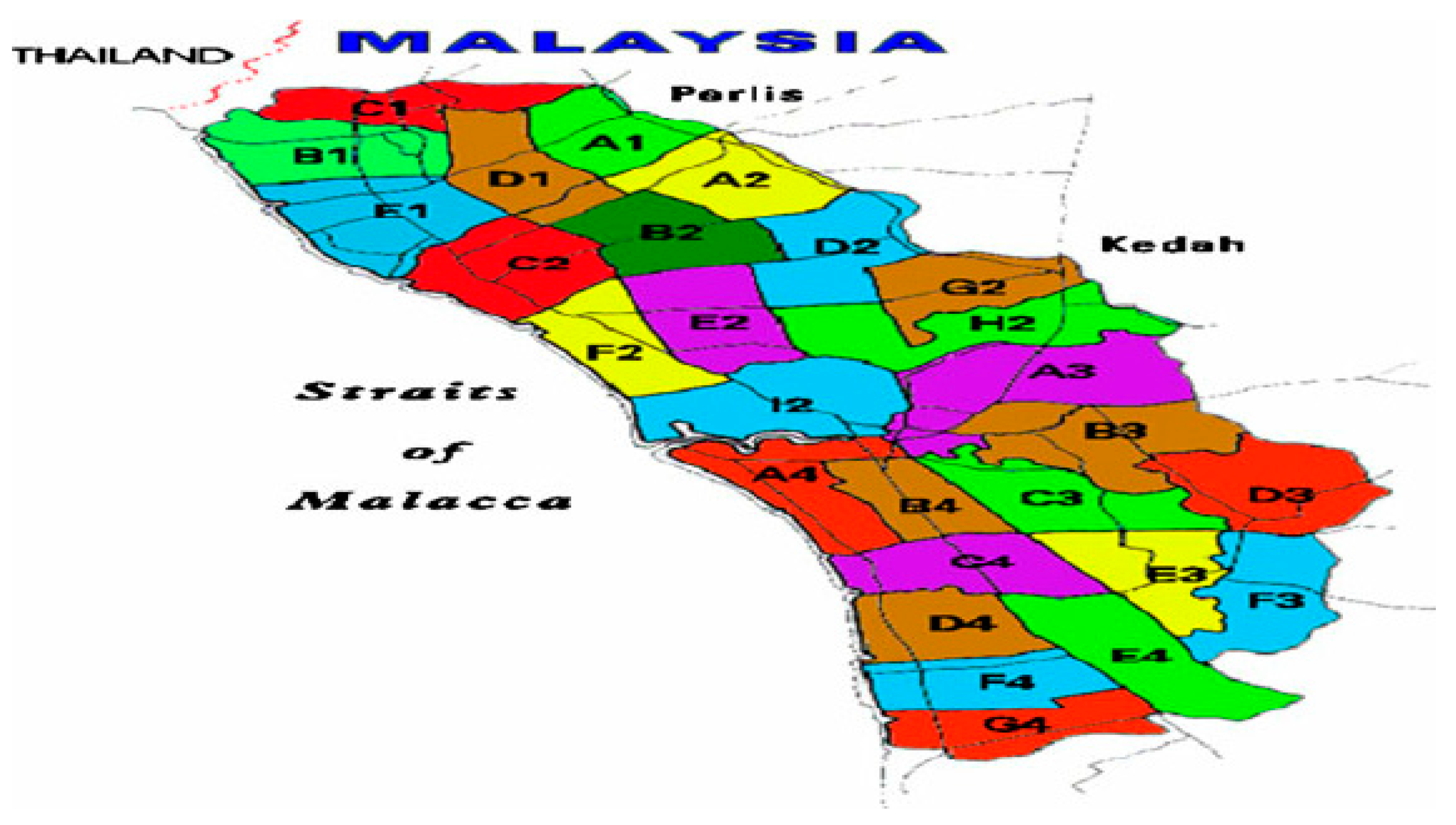
A quantitative approach was applied for this study and for this purpose secondary data were collected from 1970 to 2014 on selected variables. The data include historical information about rice cultivation, rainfall, and price statistics for both main-season and off-season rice in the MADA (Muda Agricultural Development Authority). Cointegration and the vector error correction model (VECM) approach were applied to check the short-run and long-run associations among the selected variables.

3.1.1. Study Area

There are eight main rice producing areas also called eight granary areas in Malaysia. Among the eight granary areas, the MADA (Northwest Peninsular Malaysia) is the largest one where rice is dominantly grown in the Perlis and Kedah states (Figure 1). This area covers about 125,555 ha, of which 105,581 ha are located in the northwestern part and 20,304 ha are in the southern part of Perlis. Approximately 76% of the land is under paddy cultivation and around 48,500 farm families live there [30,31]. This area is known as the paddy bowl of Malaysia. Therefore, this study has been conducted in this region, and for this reason the requisite data were obtained from the MADA, which works under the ministry of agriculture.

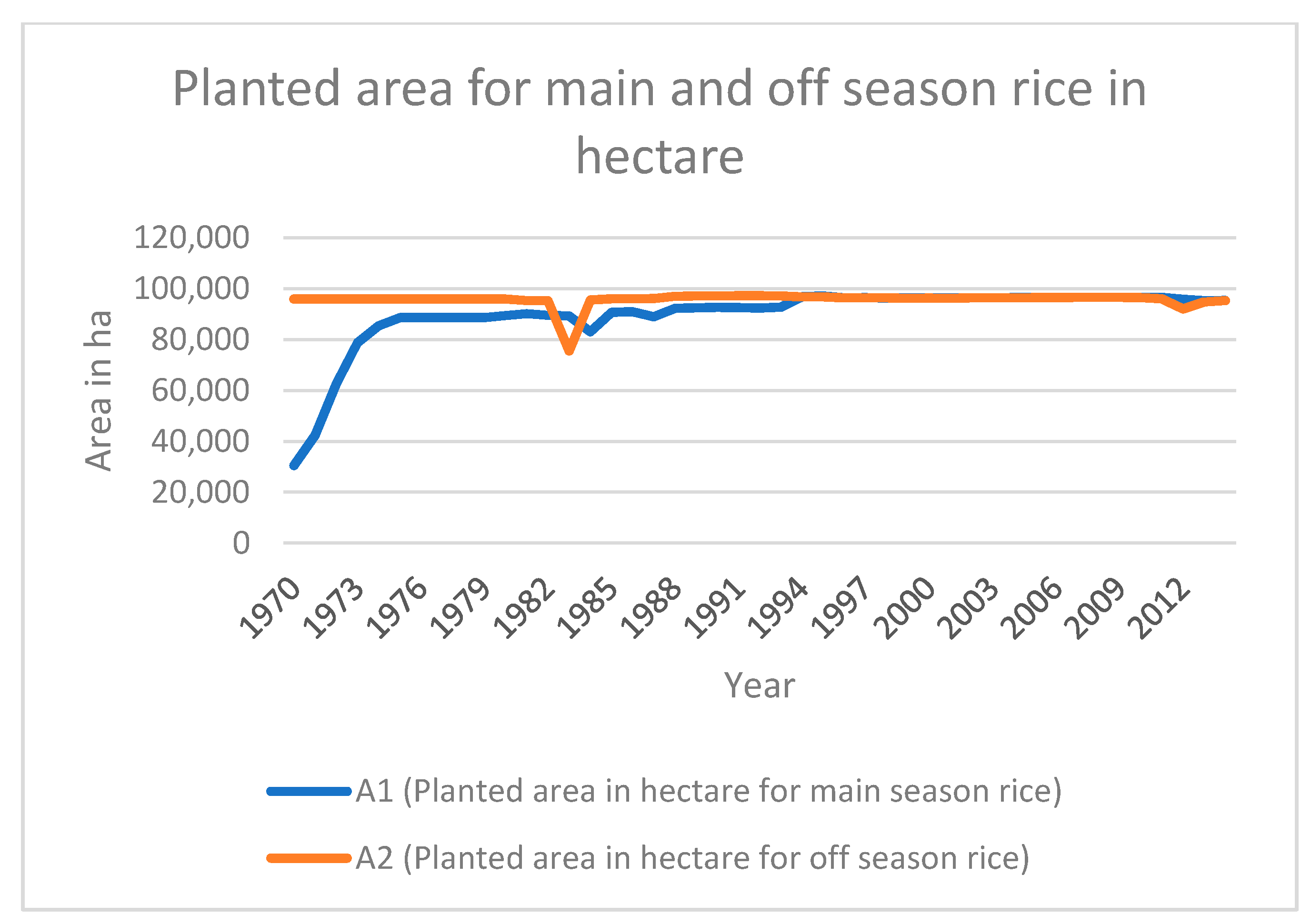
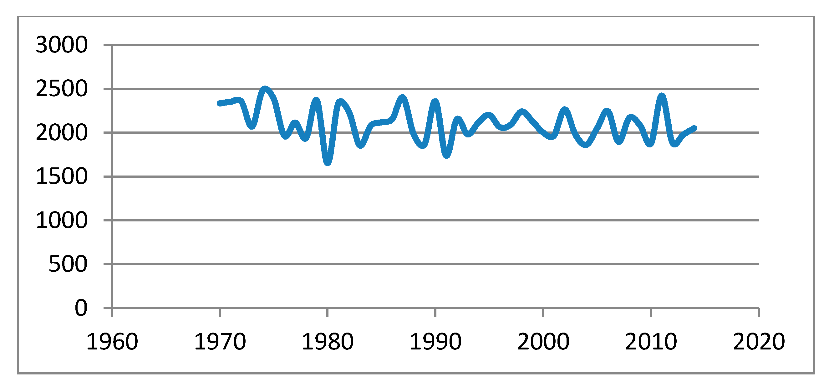
3.1.2. Rice Production System in Malaysia and Nature of Selected Variables

Malaysia is among the unique countries that take two production seasons of rice in a year, e.g., main-season rice (September to December) and off-season rice (February to May); however, planting and harvesting times vary a bit depending on the region. Despite this, Malaysia imports rice from neighboring countries. Malaysia was once a rice exporter and now the country is a net importer of rice. That is why the Malaysian rice sector is one of the most highly regulated industries as compared to other annual and perennial crops. The country targeted an 85% self-sufficiency level by 2020 as compared to 65% in 2012 through the revival of 18,200 hectares of abandoned land to get 73,000 MT of rice in 2020 to substitute the 160,000 MT of imported rice annually [32].

The descriptive statistics of the study are given in

Table 1. Descriptive statistics of selected variables.

Item.	Y1	Y2	P1	P2	A1	A2	Rainfall
Mean	4666.23	4748.42	65.52	66.25	89,623.62	96,193.91	2106.96
Maximum	6595.00	6452.00	144.81	144.81	97,078.00	97,200.00	2487.45
Minimum	2663.00	3156.00	26.10	27.37	30,565.00	95,749.00	1652.08
Std. Dev.	1031.12	717.06	15.65	15.53	13,176.59	522.10	196.24

Note: P1 denotes production of rice in kg per hectare for main season, Y2 denotes production of rice in kg per hectare for off season, P1 denotes output price of rice in Ringgit Malaysia (RM) per 100 kg for main season, P2 denotes output price of rice in Ringgit Malaysia (RM) for off season, A1 denotes planted area of rice for main season, A2 denotes production of rice and planted area in hectares for off season.

below.

It can be verified from Table 1 that mean production, price, and planted area for off-season rice is higher than main-season rice. However, the hottest (lowest rainfall) year with a minimum rainfall of 1652.08 mm was recorded in 1980, whereas the coldest (maximum rainfall) year was in 1974 with a maximum rainfall of 2487.456 mm.

The minimum production of rice was the 2663 kg per hectare that was produced in 1983 and the maximum production of rice occurred in 2013 at 6595 kg per hectare. Mean production was 4666.23 with a standard deviation of 1031.12. The minimum and maximum off-season rice production was 3156 kg/ha and 6452 kg/ha, respectively, in 1983 and 2013. The mean production of off-season rice was 4748.42 with a standard deviation 717.065. Off-season rice mean production was higher than main season as can be seen in Figure 2.

The minimum planted area of the main-season rice was 30,565 hectares that was planted in 1970 and the maximum planted area of main-season rice was 97,078 hectares planted in 1995. The mean planted area was 89,623.62 with a standard deviation of 13,176.59. The minimum and maximum off-season planted area was 75,549 and 97,200, respectively, in 1983 and 1992. The mean planted area of off-season rice was 96,193.91 with a standard deviation 522.10. Similar to production and price, the off-season rice mean planted area was higher than main-season rice, as can be seen in Figure 3.

The minimum price of rice was in Ringgit Malaysia (RM) 26.1 per 100 kg that was given in 1972 and the maximum price of main-season rice was given in 2014 at RM 144.91. The mean price was 65.52 with a standard deviation of 15.65. The minimum and maximum off-season rice price was 27.37 and 144.81, respectively, in 1972 and 2014. The mean price of off-season rice was 66.25 with a standard deviation of 15.65. Similarly, the off-season rice mean price was higher than main-season rice, as can be seen the Figure 4.

The average annual rainfall of Malaysia in the MADA area was 2106.966 mm with a standard deviation of 196.2435 mm. However, the hottest (lowest rainfall) year with a minimum rainfall of 1652.08 mm was recorded in 1980, whereas the coldest (maximum rainfall) year was in 1974 with a maximum rainfall of 2487.456 mm, as can be seen in Figure 5.

Correlation among the selected variables given in

Table 2. Correlation matrix.

	Y1	A1	P1	P2	Y2	A2	Rainfall
Y1	1.0000
A1	0.3904	1.0000
P1	0.7744	0.3709	1.0000
P2	0.7932	0.3727	0.9730	1.0000
Y2	0.6534	0.5183	0.6457	0.6665	1.0000
A2	0.1628	0.0363	−0.0083	−0.0028	0.3503	1.0000
Rainfall	−0.1879	−0.3385	−0.2088	−0.1897	−0.2184	0.1842	1.0000

Note: all variables defined in Table 1.

shows positive as well as negative associations among different variables. It is clear that the output of season 1 (main-season) rice was highly-to-moderately and positively correlated with the price of paddy rice in season 1 as well as in season 2 (off-season). There was a moderate correlation between the area under season 1 rice and output of season 1 rice. Similarly, the price of season 1 rice was moderately and positively correlated with the output of off-season rice, as was true in case of price of season 2 rice.

3.2. Model Specification

The basic assumption in time series analysis is that variables in regression analysis must be stationary. It means that a stationary variable must have a time-invariant finite variance while it fluctuates around a constant long-run mean. Additionally, a stationary variable is the one that diminishes as lag length increases in a theoretical correlogram. Regression generates spurious results when variables are non-stationary since the variables change over time and, thus, the ordinary least squares (OLS) is ruled out [33]. Consequently, unit root and cointegration tests are required for conventional time series analyses before any estimation is performed. Under such circumstances, relying on the simple correlation matrix would lead to spurious findings as well as faulty conclusions. For this purpose, time series analytics involving the vector error correction model along with augmented Dicky–Fuller (ADF) and Phillips–Perron (PP) tests are performed to determine the exact lag length, stationarity, and elasticities.

In the model, we used the production of main- and off-season rice as dependent variables for two models, respectively, with a set of price (own price and cross-price) and non-price factors (planted area and rainfall) as independent variables. The long-run supply response is given below:

$$Y{1}_t={\beta }_o+{\beta }_{1}A{1}_t+{\beta }_{2}P{1}_t+{\beta }_{3}P{2}_t+{\beta }_4{R}_t+{\mu }_t$$

(1)

where Y1 is production of rice in kg per hectare for the main season, A1 is the planted area of rice for the main season, P1 is the output price of rice in Ringgit Malaysia per 100 kg for the main season, and P2 is the output price of rice in RM per 100 kg for the off season, R is the rainfall, $\beta$s are the parameters of the selected variables, and μ is a disturbance term. For main-season rice (season 1), we took own price as well as the price of the previous season (off-season output price of season 2 as a proxy of cross-price elasticity) output price. The purpose was to check if either price of one season significantly affected the other season’s output or not.

Similarly, the study incorporated the output supply for off-season rice production using same variables as for the main-season crop. However, Y2 and A2 are the production of rice and planted area in hectares for off-season rice, respectively. The estimated model is given by:

$$Y{2}_t={\beta }_o+{\beta }_{1}A{2}_t+{\beta }_{2}P{1}_t+{\beta }_{3}P{2}_t+{\beta }_4{R}_t+{\mu }_t$$

(2)

3.2.1. Augmented Dickey–Fuller and Phillips–Perron Stationary Tests

To formally analyze the time series data, unit root tests (augmented Dickey–Fuller and Phillips–Perron) were undertaken firstly to check the stationarity of the variable and also its order of integration, both with and without a deterministic trend. If a variable comes out non-stationary, there is a need to make it stationary through differencing technique [34,35]. The purpose is to make the variables integrated of the same order. The order of integration of the variable comes through the number of times that a variable needs differencing. By using this method, stationarity can be achieved, which is the main assumption of the time series analysis [36,37].

The following hypotheses were formulated to see if either variable was stationary or not;

H_o: $\varnothing =0$, i.e., variable has a unit root (non-stationary)

H_a: $\varnothing <0$, i.e., variable has no unit root (stationary)

The ADF test was performed by the following ordinary least squares relationship:

$$\Delta y_t={\alpha }_o+{\beta }_t+\varnothing y_{t-1}+{\displaystyle \sum }_{i=1}^p{\delta }_i\mathsf{\Delta }{y}_{t-i}+{\epsilon }_t$$

(3)

where $\alpha$ and β are constants, t is a deterministic trend, p is the lag order selected based on Schwarz Bayesian criterion (SBC). The null hypothesis is non-stationarity, whereas rejection is stationarity situation (p-value less than 5% level of significance). Similarly, the Phillips–Perron test, which is a non-parametric test, was applied as an alternative to ADF.

3.2.2. Johansen-Juselius Cointegration Test

The cointegration test was applied to check the long-run associations among the selected variables. For this purpose, the Johansen [38] and Johansen and Juselius [39] JJ-model was applied. The JJ procedure provides a unified framework for estimation and testing of cointegrating relations in the context of VAR error correction models. In a system of r variables, there can be up to r − 1 linearly independent cointegrating vectors. The JJ multivariate cointegration model can be represent as:

$$\mathsf{\Delta }{y}_t={\alpha }_o+\mathsf{\Pi }{y}_{t-1}+{\displaystyle \sum }_{i=1}^{p-1}{\mathsf{\Psi }}_i\mathsf{\Delta }{y}_{t-1}+{\epsilon }_t$$

(4)

where, $\mathsf{\Pi }$ and $\mathsf{\Psi }$ are the coefficient matrices, p is the lag order selected based on SBC, and $\mathsf{\Delta }$ is the symbol of difference operator. The JJ model uses two criterion: trace statistics and maximum eigenvalue, to check the order of cointegration [40,41]. In a system of r variables, there can be up to r − 1 linearly independent cointegrating vectors such as:

Trace statistics:

$${\lambda }_{Trace}\left(r\right)=-n{{\displaystyle \sum }}_{i=r+1}^m\ln \left(1-{\lambda }_t^{^}\right)$$

(5)

Maximum eigenvalue:

$${\lambda }_{max}=\left(r,r+1\right)=-nln\left(1-{\lambda }_{t+1}^{^}\right)$$

(6)

where, n is the sample size and ${\lambda }_t^{^}$ is the expected eigenvalue of the characteristic roots. The null hypothesis was no cointegration between the series of the variables (r = 0) against the alternative hypothesis that there was one cointegrating vector/relation between the variables (r = 1). Therefore, we can move to the VECM scheme if the variables are found to be cointegrated after applying the JJ test. This simply means that there exists a long-run association among the selected variables. The optimum lag length was selected before implementing the JJ test. The AIC and LR were applied to determine the system lag order (

Table 3. Lag Selection.

Lag	LogL	LR	FPE	AIC	SC
0	−1348.905	NA	6.88e+21	64.47168	64.67855
1	−1226.416	209.9817	6.69e+19 *	59.82933 *	61.07052 *
2	−1214.544	17.52589	1.32e+20	60.45446	62.72998
3	−1182.419	39.77391 *	1.08e+20	60.11517	63.42501

* indicates lag order selected by the criterion, LR: sequential modified LR test statistic (each test at 5% level), FPE: final prediction error, AIC: Akaike information criterion. SC: Schwarz information criterion.

).

3.2.3. Vector Error Correction Model

Cointegration gives the causality among the selected variables, however, it does not show the direction of the causal relationship. Furthermore, the JJ model shows that the cointegration variables can be specified by an error correction mechanism (ECM) that can be estimated by applying standard methods and diagnostic tests. Error correction term (ECT) tells us the adjustment speed with which a model returns to equilibrium following an exogenous shock, such as:

$$EC{T}_{t-1}=y_{t-1}-{\alpha }_o{\epsilon }_o-{\alpha }_1{x}_{t-1}$$

(7)

The coefficient of ECT must be negative and statistically significant, which shows the long-run causality. In our models, $(Y1-{\theta }_{1}A1-{\theta }_{2}P1-{\theta }_{3}P2-{\theta }_4\mathrm{R}$) and $\left(Y2-{\theta }_{1}A2-{\theta }_{2}P1-{\theta }_{3}P2-{\theta }_4\mathrm{R}\right)$ are the ECT for both models, e.g., main- and off-season rice. The VECM model for rice output was estimated as given as under:

$$\begin{array}{ll}\mathsf{\Delta }Y{1}_t={\beta }_{10}+& {\displaystyle \sum }_{i=1}^n{\beta }_{11i}\mathsf{\Delta }Y{1}_{t-i}+{\displaystyle \sum }_{i=1}^n{\beta }_{12i}\mathsf{\Delta }A{1}_{t-i}+{\displaystyle \sum }_{i=1}^n{\beta }_{13i}\mathsf{\Delta }P{1}_{t-i}+{\displaystyle \sum }_{i=1}^n{\beta }_{14i}\mathsf{\Delta }P{2}_{t-i}+{\displaystyle \sum }_{i=1}^n{\beta }_{15i}\mathsf{\Delta }{R}_{t-i}+\\ & {\delta }_1{(Y1-{\theta }_{1}A1-{\theta }_{2}P1-{\theta }_{3}P2-{\theta }_{4}R)}_{t-1}+{\omega }_t\end{array}$$

(8)

$$\begin{array}{ll}\mathsf{\Delta }Y{2}_t={\beta }_{20}+& {\displaystyle \sum }_{i=1}^n{\beta }_{21i}\mathsf{\Delta }Y{2}_{t-i}+{\displaystyle \sum }_{i=1}^n{\beta }_{22i}\mathsf{\Delta }A{2}_{t-i}+{\displaystyle \sum }_{i=1}^n{\beta }_{23i}\mathsf{\Delta }P{1}_{t-i}+{\displaystyle \sum }_{i=1}^n{\beta }_{24i}\mathsf{\Delta }P{2}_{t-i}+{\displaystyle \sum }_{i=1}^n{\beta }_{25i}\mathsf{\Delta }{R}_{t-i}+\\ & {\delta }_2{(Y2-{\theta }_{1}A2-{\theta }_{2}P1-{\theta }_{3}P2-{\theta }_{4}R)}_{t-1}+{\nu }_t\end{array}$$

(9)

where, ${\beta }_{11}\mathrm{and}{\beta }_{22}$ are the short-term coefficients, ${\delta }_1,\mathrm{and}{\delta }_2,$ are the long-run speed of adjustment coefficients, and ${\omega }_t,{\nu }_t$ are the stochastic error terms. All other variables have been previously defined. The whole analysis was performed using the EViews statistical software.

4. Results and Discussion

4.1. Unit Root Tests

For a long-run relationship to be viable, it is important to find the unit root test with and without trend. If the used variables are non-stationary, the regression results will be spurious, and any long-run relationship will be nonsense in unit root test [36,38]. Most of the variables are non-stationary, as can be seen in

Table 4. Unit root test for selected variables.

	ADF Unit Root Test		PP Unit Root Test
At Level	Without Trend	With Trend	Without Trend	With Trend
Production Season 1	−1.23 (0.652)	−2.443 (0.354)	−0.702 (0.836)	−2.311 (0.419)
Production Season 2	−3.182 (0.028) **	−5.468 (0.000) *	−3.182 (0.027) **	−5.454 (0.000) *
Planted Area for Season 1	−4.095 (0.003) *	−14.25 (0.000) *	−16.06 (0.000) *	−14.26 (0.000) *
Planted Area for Season 2	−6.02 (0) (0.000) *	−6.01 (0) (0.000) *	−6.02 (1) (0.000 )*	−6.01 (0) (0.000) *
Rainfall	−5.49 (0) (0.000) *	−6.17 (1) (0.000) *	−8.48 (4) (0.000) *	−9.46 (3) (0.000) *
Price Season 1	−1.12 (0) (0.697)	−4.24 (0) (0.008) *	−0.67 (3) (0.844)	−4.26 (3) (0.008) *
Price Season 2	−0.77 (0) (0.817)	−4.76 (0) (0.002) *	−0.36 (2) (0.907)	−4.75 (3) (0.002)
First Difference
Production Season 1	−7.099 (0.000) *	−6.178 (0.000) *	−7.549 (0.000) *	−8.413 (0.000) *
Production Season 2	−9.98 (0.000) *	−9.86 (0.000) *	−31.67 (0.000) *	−32.79 (0.000) *
Planted Area for Season 1	−9.28 (0.000) *	−8.33 (0.000) *	−6.76 [8] (0.000) *	−5.00 [7] (0.001) *
Planted Area for Season 2	−10.81 (0) (0.000) *	−10.68 (0) (0.000)	−34.94 (34) (0.000) *	−34.41 (34) (0.000) *
Rainfall	−11.12 (1) (0.000) *	−11.01 (1) (0.000) *	−15.99 (1) (0.000) *	−15.82 (1) (0.000) *
Price Season 1	−7.92 (0) (0.000) *	−7.97 (0) (0.000) *	−9.30 (9) (0.000) *	−9.68 (9) (0.000) *
Price Season 2	−8.33 (0) (0.000) *	−8.49 (0) (0.000) *	−8.97 (5) (0.000) *	−9.26 (5) (0.000) *

Note: The asterisks ** and * denote significance at 5% and 10% levels, respectively.

. However, once first differences were taken, all variables became stationary at one percent level of significance using ADF and PP unit root creation.

The JJ model indicated that cointegration or a long-term relationship exists among the variables under consideration such as production of main-season rice, planted area of main season, price of rice for season 1 and two, and rainfall from 1970–2014. The trace test and max-eigen statistics indicate two cointegrating eqn(s) at the 0.05 level, as can be seen in

Table 5. JJ model for main-season rice.

Hypothesized No. of CE(s)	Trace Statistic	0.05 Critical Value	Prob.	Result
None	160.7152	69.81889	0.0000 **	Cointegration
At most 1	73.64125	47.85613	0.0000 **	Cointegration
At most 2	27.72313	29.79707	0.0852	No Cointegration
At most 3	8.519340	15.49471	0.4117	No Cointegration
At most 4	0.039798	3.841466	0.8418	No Cointegration
Hypothesized CE(s)	Max-Eigen Stat	0.05 Critical Value	Prob.	Result
None	87.07400	33.87687	0.0000 **	Cointegration
At most 1	45.91812	27.58434	0.0001 **	Cointegration
At most 2	19.20379	21.13162	0.0911	No Cointegration
At most 3	8.479542	14.26460	0.3320	No Cointegration
At most 4	0.039798	3.841466	0.8418	No Cointegration

Note: ** show Trace test max eigen statistics that point out two cointegrating eqn(s) at the 0.01 level.

below.

4.2. JJ Model for Main- and Off-Season Rice Production

Similarly, the JJ model for off-season rice indicated that a long-term relationship also exists among the variables under consideration, which can be seen from the trace test and max-eigen statistics. This shows that at least two cointegrating equations exist at the 0.05 level under trace statistics, however, at least one cointegration equation exists at the 5% level under max-eigen statistics, as can be seen in

Table 6. JJ model for off-season rice.

Hypothesized CE(s)	Trace Statistic	0.05 Critical Value	Prob.	Result
None	100.7561	69.81889	0.0000 **	Cointegration
At most 1	52.65720	47.85613	0.0165 **	Cointegration
At most 2	29.07682	29.79707	0.0604	No Cointegration
At most 3	10.87743	15.49471	0.2191	No Cointegration
At most 4	0.095572	3.841466	0.7572	No Cointegration
Hypothesized CE(s)	Max-Eigen Stat	0.05 Critical Value	Prob.	Result
None	48.09888	33.87687	0.0006 **	Cointegration
At most 1	23.58038	27.58434	0.1500	No Cointegration
At most 2	18.19939	21.13162	0.1226	No Cointegration
At most 3	10.78186	14.26460	0.1655	No Cointegration
At most 4	0.095572	3.841466	0.7572	No Cointegration

Note: ** show Trace test statistics depicting two cointegrating eqn(s) at the 0.05 level while max-eigenvalue test shows one cointegrating eqn(s) at the 0.01 level.

below.

From these findings, we can say that enough evidence is present that long-term associations exist among the variables under two different models. Hence, we can move for the long-run and short association for two models.

4.3. Long-Run and Short-Run Association between Rice Supply and Relative Price

The estimated coefficient of the one-lagged error correction term ($EC{T}_{t-1}$) was statistically significant and carried the negative sign as expected. This provided evidence that there is an equilibrium relationship that exists between rice supply (production) and its relative price. The coefficient of −0.204 shows that about 20.4% of the variation of rice supply from the long-run equilibrium level is corrected biannually, as shown in the

Table 7. Long- and short-run estimates.

Long-Run Estimates (Normalized on Y1) Model 1		Long-Run Estimates (Normalized on Y2) Model 2
Constant	340.27	Constant
$\mathit{A}{\mathbf{1}}_{\mathit{t}}$	4.91 (1.89)	$\mathit{A}{\mathbf{2}}_{\mathit{t}}$	−1.34 (1.04)
$\mathit{P}{\mathbf{1}}_{\mathit{t}}$	−0.558 (0.71)	$\mathit{P}{\mathbf{1}}_{\mathit{t}}$	−1.32 (0.37)
$\mathit{P}{\mathbf{2}}_{\mathit{t}}$	0.71 (0.74)	$\mathit{P}{\mathbf{2}}_{\mathit{t}}$	1.64 (0.36)
${\mathit{R}}_{\mathit{t}}$	−782 (1.80)	${\mathit{R}}_{\mathit{t}}$	0.98 (0.70)
Short-run Estimates
$\mathit{A}{\mathbf{1}}_{\mathit{t}-\mathbf{3}}$	1.55 * (3.39)	$\mathit{A}{\mathbf{2}}_{\mathit{t}-\mathbf{1}}$	−2.45 * (−2.98)
$\mathit{P}{\mathbf{1}}_{\mathit{t}}$	0.04 (0.24)	$\mathit{P}{\mathbf{1}}_{\mathit{t}}$	0.05 (0.33)
$\mathit{P}{\mathbf{2}}_{\mathit{t}}$	−0.22 (−0.92)	$\mathit{P}{\mathbf{2}}_{\mathit{t}}$	−0.026 (−1.49)
${\mathit{R}}_{\mathit{t}}$	0.95 ** (2.07)	${\mathit{R}}_{\mathit{t}}$	0.76 ** (2.28)
$\mathit{E}\mathit{C}{\mathit{T}}_{\mathit{t}-\mathbf{1}}$	−0.204 * (−2.77)	$\mathit{E}\mathit{C}{\mathit{T}}_{\mathit{t}-\mathbf{1}}$	−0.832 * (−2.98)
Diagnostic Tests
R2	0.6013	R2	0.4588
BG-LM(3)	0.876 [0.469]	BG-LM(2)	1.22 [0.28]
JB	4.52 [0.11]	JB	4.52 [0.11]
Heteroskedasticity	0.846 [0.642]	Heteroskedasticity	0.40 [0.97]

Note: **, and * denote significance at 5%, and 10% levels, respectively. Figures in parenthesis (…) are t-statistics while figures in brackets […] are p-values.

. This depicts that any short-run deviation will take about 2.5 years to adjust to long-run equilibrium. This is a very slow adjustment. On the other hand, ($EC{T}_{t-1}$) showed that output adjustment towards the long-run equilibrium for model two was also negatively significant i.e., −0.83 (Table 7, model 2). The coefficient of −0.832 shows that there was only about 83.2% of the deviation of rice supply for off-season. Hence, any short-run deviation would take about one-and-a-half years to adjust to long-run equilibrium. This might be possible as rice is an annual crop and especially since there are two production seasons in Malaysia, so almost after three production season it can be adjusted to long-run equilibrium. On the other hand, Sehar et al. [42] found the error correction term with the coefficient value of 0.499, which means it takes two years to adjust to the equilibrium.

The short-run elasticities with respect to the relative planted area and rainfall were consistent with priori expectations in terms of both magnitudes and signs; the short-run elasticity of the planted area was 1.55 and for rainfall was 0.95. A previous study on Malaysia found that lagged one-year area is negatively linked to paddy supply and lagged two-year area is substantially and positively linked to supply [43], while in this study the planted area for one lag was stronger and carried a coefficient value of 1.55. Similarly, the coefficient value of rainfall was 0.95. which depicted that every 1% increase in rainfall would result in a 95% increase in rice output within the country. These results can be compared with the Lee et al. study where they found an inelastic effect as the lagged one-year rain variable’s coefficient was less than one unit. This is very important in a Malaysian context as the country’s geographical location is not compatible with irrigation systems as compared to other developed countries. Therefore, Malaysian farmers need enough rainfall as rice is not able to fully depend on the country’s irrigation system [44]. These results are in accordance with a past study where Farhan et al. [45] found that land area positively and significantly affects output supply. However, Khan et al. [29], in the case of Pakistani rice, showed a short-run elasticity of 0.597 for production, 0.037 for price, and −0.066 for competitive crop (maize), showing the inelastic relation of production with lag production, lag price, and lag competitive crop price.

In the same way, the short-run elasticities represented in model 2, which can be seen in the left two columns in Table 7, showed that rainfall was exactly according to a priori expectation in terms of sign and magnitude; however, planted areas have a negative sign. This might be due to the fact the production in the off season gives less returns on rice and farmers have the incentive to move part of the land in favor of other productive crops. The coefficient of the planted area was −2.45 and significant, while for rainfall it was 0.76, i.e., positive and significant. A study conducted in Ghana showed somewhat contrasting elasticities with respect to rainfall, competitive crop price, and lagged output [13]. It showed that the land area cultivated under rice was significantly dependent on output, rainfall, real price of maize, and real price of rice. The elasticity for rainfall under the Ghanaian context was 0.004, much lower than in the case of Malaysia.

As noted by Hallam and Zanoli [46] and Hendry et al. [47], a general autoregressive distributed lag model encapsulates both the Nerlovian partial adjustment model and the VECM model. For short-run causalities between productions for season 1 and independent variables (IVs), Wald statistics can be used. A Wald test showed that (Chi-square = 12.32, p = 0.0064) there was a short causality from the planted area to production for season 1. Similarly, a Wald test for the price of season-1 rice showed that there was no short-run causality (p = 0.93, Chi-square = 0.42). However, a Wald test for the rainfall showed that there was a short-run causality (p = 0.02, Chi-square = 9.76). Hence, based on the above decision, the study concluded that there was a long-run causality from IVs to production for season 1 and there was also a short causality that existed between production and planted area and rainfall. Thus, the VECM is the better way to describe the data than the partial adjustment model. These findings are in agreements with the results of previous studies [42,48] for various crops.

The response of the lagged planted area of main-season rice (1.55) in the short run was significant at 1%, but the long-run elasticity was not significant for both main- and off-season rice. Similarly, the elasticity of the lagged planted area of off-season rice in the short run was −2.45, which was significant at 1 percent. The lagged planted areas were used as a proxy for experience. The reason for this is farmers increase/decrease their planted areas for main- and off-season rice based on experience. Main-season rice was found to be more productive and profitable, implying that farmers’ experience played a role in the productivity of rice. The previous experience of rice farmers influenced their decision to grow rice in the main season. Therefore, farmers’ lagged planted area (experience) is positively and significantly associated with output. Contrary to this, the lagged planted area of off-season rice showed a negative and significant association with rice output. This may be due to the fact that farmers usually leave the lands unplanted to get more output in the main season. The previous year’s planted area had a significant effect on farmers’ decisions to allocate more land for main-season rice (model 1) and less land for off-season rice (model 2). The results were justified in a past study where Abraham and Pingali [11] found that experience has a positive impact on the supply response of various crops in India.

Rainfall is the crucial component of rice production in Malaysia as irrigation infrastructure is very poor and somewhere scant in the country. Rainfall had significant effects on the production of rice for both seasons at a 5% level of significance. This low impact of rainfall can be explained by the fact that a large proportion of total rice output is produced under only the rainfall across the country and irrigation water infrastructure is poor. Therefore, there is need to supply plenty of water through irrigation systems as there is fear of a shortage of water due to erratic rainfall and climate change in Malaysia. The results of this study can be supported from the past studies [25,49].

It can be seen from the two models (both for main-season and off-season rice) that price factors are poor and insignificant, and non-price factors such as planted area and rainfall are strongly related with the supply of rice. It is clear from the results that erratic rainfall may reduce the output but continuous increase in rainfall can increase the supply of rice as average rainfall has decreased in Malaysia from 1970 to 2014. These results are in agreement with previous studies where research found that non-price factors are more prevalent in determining the supply of various crops as compared to price factors [10,26].

Based on AIC and LR criterions, maximum lag was selected, which is three, while for model 2 it was one. The speed of adjustment toward a long-run average should be significant and negative, as our results showed. This means that there is a long-run causality from the IVs, which shows that IVs influence the dependent variables (DVs) such as production in the long run. Simply put, there is a long-run casualty coming from IVs to production for season 1. Hence, the results were acceptable. Whether our model where production is a DV has any statistical error or not, it can be judged by R², which was 60.14, and F-statistic, which was 2.26, with p = 0.03. This means that the model was good fit at a five percent level of significance. Further, this model is free from serial correlation. Results also showed that there was no heteroskedasticity in the model. Residual of this model were also normally distributed, as can be seen in Table 7 regarding the Jarque–Berra (JB) test.

The models were a good fit concerning adequacy, as can be seen in lower part of Table 7. For instance, the JB statistic showed that the residuals were normally distributed while the Breusch–Godfrey LM (BG-LM) test reported that there was no issue of autocorrelation. Also, the assumption of homoskedasticity was justifiable, as suggested by tests for ARCH residuals [39,50].

5. Conclusions

This study used a cointegration approach to find the supply response of rice in relation to both price and non-price factors. The study found that enough rainfall instead of erratic downfall is the main predictor of rice supply in Malaysia, suggesting proper availability of water is needed for the sustainability of rice production. This is the main factor that will help Malaysia to achieve the self-sufficiency level of 100 percent rice production and no dependency on imported rice. Main-season rice production was once higher than off-season production, however, things reversed after 1990. This might be the reason that the speed of adjustment for main-season rice production is rather slow (2.5 years) as compared to off-season rice production (about one-and-a-half years). Moreover, the correlation matrix also showed this trend. For instance, there was a positive correlation between production of season 1 (main-season rice) and season 2 (off-season rice). The Same is true for production area. The area of production of season 1 positively correlated with the production of season 2. This means that informed policy makers should ensure the plantation of rice in both seasons and try not to leave rice areas unplanted. This study only checked the correlation matrix; however, future studies can perform cointegration tests on these. Additionally, lagged planted area (proxy for experience) is another important factor to determine the rice supply. Lagged planted area increased supply of rice for both main- and off-season rice. Therefore, this study suggests that there should be an increase in rice planting area through the revival of abandoned land. Moreover, the findings of this study imply that commodity price has a weak impact on the supply of rice; rather, factors other than price such as planted area and rainfall have been more conspicuous in terms of rice productivity. This finding advocates for an increased capacity to help rice farmers through easy access to information and skill development while urging them to use additional areas for rice farming to ensure an uninterrupted supply of food grains in the country. This study used only rainfall and planted area as non-price factors; however, future research can be done on rice supply response by taking other non-price factors such as infrastructure availability, technology usage (e.g., climatic resilient and water resistant varieties), labor, and fertilizer. Furthermore, other studies can also incorporate price factors such as imported rice price and price of substitute crops. Future studies can also incorporate the impact of rainfall on different growth stages of rice in addition to other climatic factors such as carbon emissions.

References

1. United States Department of Agriculture. Malaysia Grain and Feed Annual 2017; Food and Agriculture Organization of the United Nations, Regional Office for Asia and the Pacific: Bangkok, Thailand, 2017. Available online: https://gain.fas.usda.gov/Recent%20GAIN%20Publications/Grain%20and%20Feed%20Annual_Kuala%20Lumpur_Malaysia_3-27-2017.pdf (accessed on 1 March 2018).
2. Food and Agriculture Organization of the United Nations. Food and Agriculture Crops Production by Country; Food and Agriculture Organization of the United Nations: Rome, Italy, 2018; Available online: http://www.fao.org/faostat/en/#data/TP (accessed on 29 June 2018).
3. Ruzmi, R.; Ahmad-Hamdani, M.S.; Abidin, M.Z.Z.; Burgos, N.R. Evolution of imidazolinone-resistant weedy rice in Malaysia: The current status. Weed Sci. 2021, 2021, 1–34. [Google Scholar] [CrossRef]
4. Department of Statistic Malaysia (DOSM). Selected Agriculture Indicators, Strategic Communication and International Division; Department of Statistic Malaysia: Putrajaya, Malaysia, 2018.
5. FAO. Selected Indicators of Food and Agriculture Development in Asia-Pacific Region 1992–2002; Food and Agriculture Organization of the United Nations, Regional Office for Asia and the Pacific: Bangkok, Thailand, 2011. [Google Scholar]
6. Huang, H.; von Lampe, M.; van Tongeren, F. Climate change and trade in agriculture. Food Policy 2017, 36, S9–S13. [Google Scholar] [CrossRef]
7. Thiele, R. Estimating the Aggregate Agricultural Supply Response: A Survey of Techniques and Results for Developing Countries. (No. 1016), Kiel Working Paper. 2000. Available online: https://www.econstor.eu/handle/10419/2516 (accessed on 29 June 2018).
8. Yu, B.; Liu, F.; You, L. Dynamic agricultural supply response under economic transformation: a case study of Henan, China. Am. J. Agric. Econ. 2012, 94, 370–376. [Google Scholar] [CrossRef] [Green Version]
9. Kanwar, S. Relative profitability, supply shifters and dynamic output response, in a developing economy. J. Policy Model. 2006, 28, 67–88. [Google Scholar] [CrossRef]
10. Tuteja, U. Growth performance and acreage response of pulse crops: A state-level analysis. Indian J. Agric. Econ. 2006, 61, 218–237. [Google Scholar]
11. Abraham, M.; Pingali, P. Shortage of pulses in India: Understanding how markets incentivize supply response. J. Agribus. Dev. Emerg. Econ. 2018. [Google Scholar] [CrossRef]
12. Ampadu-Ameyaw, R.; Awunyo-Vitor, D. Effect of price and non-price incentives on production and marketable surplus of food crops supply in Ghana. Asian J. Agric. Exten. Econ. Sociol. 2014, 3, 666–679. [Google Scholar] [CrossRef]
13. Kuwornu, J.K.; Izideen, M.P.; Osei-Asare, Y.B. Supply response of rice in Ghana: A co-integration analysis. Interventions 2011, 2011, 2. [Google Scholar]
14. Haile, M.G.; Kalkuhl, M.; von Braun, J. Inter-and intra-seasonal crop acreage response to international food prices and implications of volatility. Agric. Econ. 2014, 45, 693–710. [Google Scholar] [CrossRef]
15. Haile, M.G.; Kalkuhl, M. Agricultural Supply Response to International Food Prices and Price Volatility: A Cross Country Panel Analysis; 2013 Annual Meeting, 4–6 August 2013, No. 149630; Agricultural and Applied Economics Association: Washington, DC, USA, 2013. [Google Scholar]
16. Subervie, J. The variable response of agricultural supply to world price instability in developing countries. J. Agric. Econ. 2008, 59, 72–92. [Google Scholar] [CrossRef]
17. Rosenzweig, C.; Liverman, D. Predicted effects of climate change on agriculture: A comparison of temperate and tropical regions. In Global Climate Change: Implications, Challenges and Mitigation Measures; Majumdar, S.K., Ed.; Pennsylvania Academy of Sciences: Philadelphia, PA, USA, 1992; pp. 342–361. [Google Scholar]
18. Chidiebere-Mark, N.; Ohajianya, D.; Obasi, P.; Onyeagocha, S. Profitability of rice production in different production systems in Ebonyi State, Nigeria. Open Agric. 2019, 4, 237–246. [Google Scholar] [CrossRef]
19. Guibao, M. Supply Response of Rice (Oryza sativa) in the Philippines. Bachelor’s Thesis, University of Southeastern Obrero, Davao City, Philippines, 2005. [Google Scholar]
20. Erazo-Hinlo, J.; Edgardo, D.C. Rice Supply Response in the Philippines: An ALMON Lag Approach; Philippine Agricultural Economics & Development Association (PAEDA): Davao City, Philippines, 2013; Available online: https://paedacon.files.wordpress.com/2013/10/fullpaper_erazohinlo_jennifer.pdf (accessed on 1 March 2018).
21. Yu, B.; Fan, S. Rice production response in Cambodia. Agric. Econ. 2011, 42, 437–450. [Google Scholar] [CrossRef]
22. Edison, A.M.; Jie, F.; Parton, K.A. The Analysis of Supply Response of Rice under Risk in Jambi Province (No. 422-2016-26966). 2011. Available online: https://www.researchgate.net/publication/254385640 (accessed on 1 March 2018).
23. Kongrithi, W.; Isvilanonda, S. Supply Response of Thailand’s Rice to the Price of Biofuel Crops. Appl. Econ. J. 2009, 16, 1–25. [Google Scholar]
24. He, W.; Liu, Y.; Sun, H.; Taghizadeh-Hesary, F. How Does Climate Change Affect Rice Yield in China? Agriculture 2020, 10, 441. [Google Scholar] [CrossRef]
25. Khatun, M.M.; Saha, S.M.; Khan, M.A.; Hossain, M.E. Farmers’ Supply Response and Perception of Rice Procurement Program in Bangladesh. Future Food J. Food Agric. Soc. 2020, 8, 1–12. [Google Scholar]
26. Hellen, H.B.; Mangisoni, J.; Elepu, G. Citrus supply response in Kyoga plains agricultural zone, Uganda. Afr. J. Rural Dev. 2020, 4, 431–439. [Google Scholar]
27. Rahman, A. Is Price Transmission in the Indian Pulses Market Asymmetric? J. Quant. Econ. 2015, 13, 129–146. [Google Scholar] [CrossRef]
28. Rahman, M. Factors Affecting Price Fluctuation of Rice and Exploring the Rice Market in Barishal from the Consumer and Wholesaler Point of Views. 2019. Available online: https://halshs.archives-ouvertes.fr/halshs-02275376/document (accessed on 21 April 2021).
29. Khan, S.U.; Faisal, M.A.; Haq, Z.U.; Fahad, S.; Ali, G.; Khan, A.A.; Khan, I. Supply response of rice using time series data: Lessons from Khyber Pakhtunkhwa Province, Pakistan. J. Saudi Soc. Agric. Sci. 2019, 18, 458–461. [Google Scholar] [CrossRef]
30. Raziah, M.L.; Engku, E.; Tapsir, S.; Mohd, Z. Food security assessment under climate change scenario in Malaysia. Palawija News 2010, 27, 1–5. [Google Scholar]
31. Vaghefi, N.; Shamsudin, M.N.; Radam, A.; Rahim, K.A. Impact of climate change on rice yield in the main rice growing areas of Peninsular Malaysia. Research. J. Environ. Sci. 2013, 7, 59. [Google Scholar]
32. Firdaus, R.R.; Latiff, I.A.; Borkotoky, P. The impact of climate change towards Malaysian paddy farmers. J. Dev. Agric. Econ. 2012, 5, 57–66. [Google Scholar] [CrossRef] [Green Version]
33. Granger, C.W.; Newbold, P. Spurious Regressions in Econometrics. J. Econ. 1974, 2, 111–120. [Google Scholar] [CrossRef] [Green Version]
34. Ng, C.N.; Young, P.C. Recursive estimation and forecasting of non-stationary time series. J. Forecast. 1990, 9, 173–204. [Google Scholar] [CrossRef]
35. Velasco, C. Gaussian Semiparametric Estimation of Non-stationary Time Series. J. Time Ser. Anal. 1999, 20, 87–127. [Google Scholar] [CrossRef] [Green Version]
36. Said, S.E.; Dickey, D.A. Testing for unit roots in autoregressive-moving average models of unknown order. Biometrika 1984, 71, 599–607. [Google Scholar] [CrossRef]
37. Dickey, D.A.; Fuller, W.A. Likelihood ratio statistics for autoregressive time series with a unit root. Econom. J. Econom. Soc. 1981, 1981, 1057–1072. [Google Scholar] [CrossRef]
38. Johansen, S. Statistical Analysis of Cointegration Vectors. J. Econ. Dyn. Control 1988, 12, 231–254. [Google Scholar] [CrossRef]
39. Johansen, S.; Juselius, K. Maximum Likelihood Estimation and Inference on Cointegration with Applications to the Demand for money. Oxf. B Econ. Stat. 1990, 52, 169–210. [Google Scholar] [CrossRef]
40. Raeeni, A.A.G.; Hosseini, S.H.; Moghadassi, R. How energy consumption is related to agricultural growth and export: An econometric analysis on Iranian data. Energy Rep. 2019, 5, 50–53. [Google Scholar] [CrossRef]
41. Wah, Y.W. The role of domestic demand in the economic growth of Malaysia: A cointegration analysis. Int. Econ. J. 2010, 18, 337–352. [Google Scholar] [CrossRef]
42. Sehar, H.; Jyoti, K.; Dileep, K.; She, R. Supply elasticity of major crops in Jammu region: An Engle-granger Co-integrating approach. J. Pharmacogn. Phytochem. 2019, 8, 4048–4052. [Google Scholar]
43. Lee, W.C.; Hoe, N.; Viswanathan, K.K.; Baharuddin, A.H. An Economic Analysis of Anthropogenic Climate Change on Rice Production in Malaysia. Malays. J. Sustain. Agric. (MJSA) 2020, 4, 1–4. [Google Scholar]
44. Saseendran, S.A.; Singh, K.K.; Rathore, L.S.; Singh, S.V.; Sinha, S.K. Effects of climate change on rice production in the tropical humid climate of Kerala, India. Clim. Chang. 2000, 44, 495–514. [Google Scholar] [CrossRef]
45. Farhan, A.S.; Shah, S.A. Supply response analysis of wheat growers in district Swabi, Khyber Pakhtunkhwa: farm level analysis. Sarhad J. Agric. 2019, 35, 274–283. [Google Scholar] [CrossRef]
46. Hallam, D.; Zanoli, R. Error Correction Models and Agricultural Supply Response. Eur. Rev. Agric. Econ. 1993, 20, 151–166. [Google Scholar] [CrossRef]
47. Hendry, D.F.; Pagan, A.R.; Sargan, J.D. Dynamic Specification. In Handbook of Econometrics, 2nd ed.; Griliches, Z.Z., Intriligator, M.D., Eds.; Elsevier: Amsterdam, The Netherlands, 1984; Volume 2, pp. 1023–1100. [Google Scholar]
48. Soontaranurak, K.; Dawson, P.J. Rubber acreage supply response in Thailand: a cointegration approach. J. Dev. Areas 2015, 49, 23–38. [Google Scholar] [CrossRef] [Green Version]
49. Rokonuzzaman, M.; Rahman, M.A.; Yeasmin, M.; Islam, M.A. Relationship between precipitation and rice production in Rangpur district. Progress. Agric. 2018, 29, 10–21. [Google Scholar] [CrossRef] [Green Version]
50. Horváth, L.; Teyssière, G. Empirical process of the squared residuals of an arch sequence. Ann. Statist. 2001, 29, 445–469. [Google Scholar] [CrossRef]
Figure 1. Map of MADA area. Source: Google Maps.
Agronomy 11 01463 g001
Figure 2. Production of rice in main and off seasons, 1970–2014.
Agronomy 11 01463 g002
Figure 3. Planted area of rice for main and off seasons, 1970–2014.
Agronomy 11 01463 g003
Figure 4. Prices of main- and off-season rice, 1970–2014.
Agronomy 11 01463 g004
Figure 5. Rainfall pattern in MADA area, Malaysia, 1970–2014.
Agronomy 11 01463 g005