Article

Observed Changes in Agroclimate Metrics Relevant for Specialty Crop Production in California

1
USDA California Climate Hub, Davis, CA 95616, USA
2
John Muir Institute of the Environment, University of California, Davis, CA 95616, USA
3
Division of Agriculture and Natural Resources, University of California, Merced, CA 95343, USA
4
Management of Complex Systems Department, School of Engineering, University of California, Merced, CA 95343, USA
5
USDA-ARS Sustainable Agriculture Water Systems Research Unit, Davis, CA 95616, USA
6
Civil and Environmental Engineering Department, School of Engineering, University of California, Merced, CA 95343, USA
*
Author to whom correspondence should be addressed.
Submission received: 25 November 2021 / Revised: 27 December 2021 / Accepted: 28 December 2021 / Published: 15 January 2022

Abstract

:
Every decade, a suite of standardized climatological metrics known as climate normals are updated, providing averages of temperature and precipitation data over the previous 30-year period. Although some of these climate normals are directly applicable to agricultural producers, there are additional agroclimate metrics calculated from meteorological data that provide physiologically relevant information for on-farm management decisions. In this study, we identified a suite of energy-based agroclimate metrics and calculated changes over the two most recent normal periods (1981–2010 and 1991–2020), focusing on specialty crop production regions in California. Observed changes in agroclimate metrics were largely consistent with broader global warming trends. While most metrics showed small changes between the two periods, during the 1991–2020 period, the last spring freeze occurred ~5 days earlier as compared to the 1981–2010 period, contributing to a >6 day longer frost-free period in the Sacramento and Salinas Valleys; likewise an additional 6.4 tropical nights (Tn > 20 °C) occurred in the Coachella Valley during the 1991–2020 period. A complementary trend analysis of the agroclimate metrics over the 1981–2020 period showed significant increases in growing degree days across all agricultural regions, while significant increases in heat exposure were found for the Salinas and Imperial Valleys and over the Central Coast region. Moreover, summer reference evapotranspiration increased approximately 40 mm in California’s Central Valley during 1981–2020, with implications for agricultural water resources. Quantifying the shifts in these agroclimate metrics between the two most recent 30-year normal periods and the accompanying 40-year trends provides context for understanding and communicating around changing climatic baselines and underscores the need for adaptation to meet the challenge that climate change poses to agriculture both in the future and in the present.

1. Introduction

The calculation of standardized climate metrics averaging climatological data over periods of 30 consecutive years was established by the World Meteorological Organization in 1956 and adopted by the U.S. Weather Bureau (now the National Weather Service) in the early 1960s [1,2]. These measures, known collectively as climate normals, are computed by weather stations around the world for the most recent 30-year periods and are updated once a decade (e.g., 1971–2000, 1981–2010, 1991–2020). Climate normals provide a rolling baseline for comparing observed weather conditions, calculating anomalies, and estimating likely conditions for a given place and time [3]. Given the significance of climate change, there is public interest in observed trends and comparisons between the most recent (1991–2020) normal period and the period prior (as evidenced by media attention at the time of the new normals release [4,5,6]). Relatedly, characterizing the nature of changing normals and their implications across societal sectors is a key component of improving public understanding and science communication around climate change with implications for decision-making.
In the U.S.A., the National Oceanic and Atmospheric Administration (NOAA) oversees the output of climate normals, which are released by the National Centers for Environmental Information (NCEI) and include multiple temperature and precipitation summaries at daily, monthly, seasonal, and annual time-steps, and which provide statistics including central tendency, standard deviation, frequency of exceedance, and percentiles [7]. However, these metrics alone do not capture the full picture of the climate. Climate extremes and climate variability are important drivers of ecological and societal impacts [8], and the extremes of climatic distribution can serve as important controls on the geographies of biota [9,10]. Additional summary statistics—such as the climatic extremes indices identified by the World Climate Research Program’s Expert Team on Climate Change Detection and Indices (ETCCDI)—are recommended as means for providing a more comprehensive description of the climate [2,3].
In California, where the Mediterranean-type climate and extensive water infrastructure have allowed for the cultivation of a wide variety of crops, agriculture is a >$50 billion industry. California produces forage, fiber, livestock, aquaculture, grains, and dairy, but is perhaps best known for its production of high-value specialty crops, including more than ⅓ of U.S.-grown vegetables and more than ⅔ of U.S.-grown fruits and nuts, by volume [11]. Although producer selection of crop type and variety results from a range of historical, cultural, and economic factors (e.g., [12]), climate is a primary driver of crop distribution and yield potential [13,14]. Even in highly managed agricultural systems where damage from adverse weather can be mitigated, understanding the expected conditions based on climatology can provide producers with valuable information for farm management planning (e.g., [15]). Although the climate metrics from NCEI and ETCCDI provide some utility for understanding agriculture–climate relationships, and while some of these metrics are agriculturally-relevant (e.g., ETCCDI’s number of frost days, growing degree days), there are additional climate metrics that are of interest to the agricultural community. Metrics that offer a snapshot of physiologically relevant environmental conditions and provide support for in-season decision making may be of particular importance [16], and trends in agroclimate metrics can be more useful than standard climate metrics for identifying and enacting strategies for resilient crop production and agricultural adaptation [17,18]. Likewise, there may be some advantage in communicating observed and projected climate change in terms of agriculturally relevant metrics, which presumably have more contextual meaning for agricultural producers than more widely available precipitation and temperature summaries [17].
Recognizing widely documented changes in climate both globally and across California over the last 40 years encompassing the two most recent normal periods, we anticipate that agroclimate metrics have also changed. However, a formal assessment of changes in agroclimate metrics can provide an improved understanding of recently observed climate changes in a context relevant for agricultural producers, a means of communicating around climatic baselines against which farm management decisions are made, and aid in guiding forward-looking adaptive management plans and associated investment allocation strategies at multiple scales. Given this relevance, and in light of the absence of such an assessment within the literature, we (1) analyzed changes in agroclimate metrics in California between the two most recent normal periods (1981–2010 and 1991–2020) and (2) assessed trends in the metrics over the 40-year period. We specifically focus on these changes within the context of high-value specialty crop production.

2. Data and Methods

2.1. Agroclimate Metrics
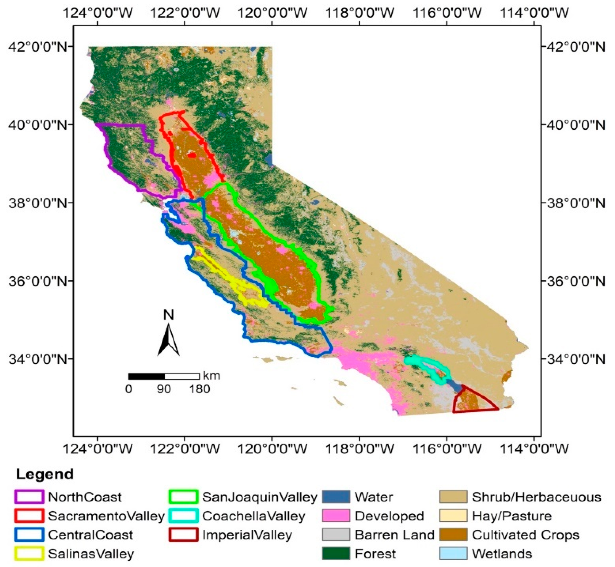
To address the need for climate metrics with specific relevance to the agricultural sector, previous studies have adapted suites of existing indices to agricultural applications (e.g., growing degree days [19]); identified a list of agroclimate metrics that are widely used and are crop specific and relevant to crop development or farm-management decisions [20,21]; and conducted literature reviews and survey assessments to determine the most used indices in research, monitoring, and modeling [22]. Likewise, prior research has sought to quantify climate impacts on agricultural production systems and identify non-meteorological indicators to assess the effects of climate variability and change on agriculture [23,24,25]. Despite the considerable previous work at the intersection of climate and agriculture, to our knowledge, there is no standardized suite of agroclimate metrics analogous to the widely used climate normals.
In the absence of a standardized set of agroclimate metrics, we selected a suite of 12 agroclimate metrics relevant to high-value California specialty crops (Table 1). These metrics were identified through a focused review of literature and agricultural decision support resources. We limited our selection to only those measures that can be derived from meteorological variables alone and that have relevance for fruit, nut, and vegetable production (i.e., biological and social indicators were not considered, nor were metrics relevant for livestock production). We focused on metrics important for crop development (e.g., chill accumulation, growing degree days) and crop stress (e.g., measures of frost and heat exposure). Furthermore, because orchard and vegetable crops account for ~50% of California’s irrigated cropland [26], we include summer reference evapotranspiration (ETo), calculated from the Penman–Monteith equation for short grass [27], as it can serve as a proxy for irrigation water demand during the peak of the growing season. However, we did not include precipitation or drought metrics in our analysis as they do not account for features of California’s agricultural water regime such as mountain snowmelt runoff, reservoir storage, water conveyance, or groundwater resources that provide a water source during otherwise dry months.

2.2. Study Area

California’s fruits, nuts, and vegetables are grown in every major agricultural region in the state and collectively cover more than 1.8 million hectares and generate ~$30 billion in cash receipts annually [11]. Most of the state’s specialty crops are cultivated across seven key regions (Figure 1). Of these, the majority of acreage is within five agricultural valleys: the Sacramento, San Joaquin, Salinas, Coachella, and Imperial Valleys. In addition, California’s north and central coasts are known for their winegrape production [52]. We have included the counties that comprise these two coastal regions (where they do not overlap with valley areas) as additional agricultural regions.

2.3. Climate Data

Daily observed maximum and minimum temperature (Tx, Tn) and reference evapotranspiration (ETo) were acquired from a ~4 km spatial resolution gridded surface meteorological dataset (gridMET; [54]) for the period 1980–2020. GridMET has demonstrated skill in capturing variability and trends in meteorological data observed at in situ stations while also containing the requisite variables for estimates of reference evapotranspiration. These data are available over the contiguous U.S.A. but were clipped to the state of California.

2.4. Difference and Trend Analysis

Each agroclimate metric was calculated at an annual time step for each 4 km gridMET cell over the 1981–2020 period. For the normal period difference analysis, we examined differences in the averages of each metric between the two 30-year periods (i.e., 1991–2020 [minus] 1981–2010). Following [55], a non-parametric Wilcoxon matched pairs test was performed to assess whether there was a significant difference (α = 0.05) between the two periods for each metric, with a null hypothesis of no significant difference; note that overlapping normal periods share 20 years in common, creating a very stringent test for significant differences. We also performed a complementary trend assessment in the metrics over the 40-year period of study using the Theil–Sen estimator. The Mann–Kendall test was used to determine statistical significance in the trends at the α = 0.05 level of significance, with a null hypothesis of no significant trend. Both the Theil–Sen and Mann–Kendall tests are non-parametric methods that do not require meeting any distribution assumptions and are commonly used in climate data trend analysis [56].
We calculated the normal period differences as a percent change and visualized these across the state but focused our reporting on the seven agricultural regions and noted the absolute change between periods in addition to the relative change. For reporting time series results, we aggregated over each of the agricultural regions. While these seven regions may also include commodity crop production, dairies, rangelands, forestlands, and urban development, we performed our analysis only over locations where high-value fruits, nuts, or vegetables are grown. Crop location data were extracted from the 30 m gridded NASS Cropland Data Layer (CDL) and were scaled to the 4 km gridMET grid, and we limit our analysis to the 4 km cells containing any cultivation of one or more specialty crops (i.e., the 4 km cell must contain at least one 30 m specialty crop pixel). Specifically, our crop mask includes locations with almonds, walnuts, winegrapes, lettuces, and tomatoes, which represent climatic, geographic, and cropping system diversity in high-value specialty crops, allowing our results to illustrate the relationships between our selected agroclimate metrics and crop production; moreover, the majority of total U.S. production of these crops comes from California, and they are economically important for the state and the regions in which they are grown (Table 2).

3. Results and Discussion

3.1. Changes between Normal Periods and Implications for Specialty Crop Production

Across geographic regions and agroclimate metrics, the differences between periods and 40-year trends were directionally consistent with warming trends. The changes in agroclimate metrics between normal periods are shown in Figure 2 and the 40-year trends in metrics are shown in Figure 3, Figure A1, Figure A2, Figure A3, Figure A4, Figure A5, Figure A6 and Figure A7; Table 3 presents metric changes (absolute and relative), trends, and significance. We highlight notable results by region below and call attention to the implications for regional specialty crop production.

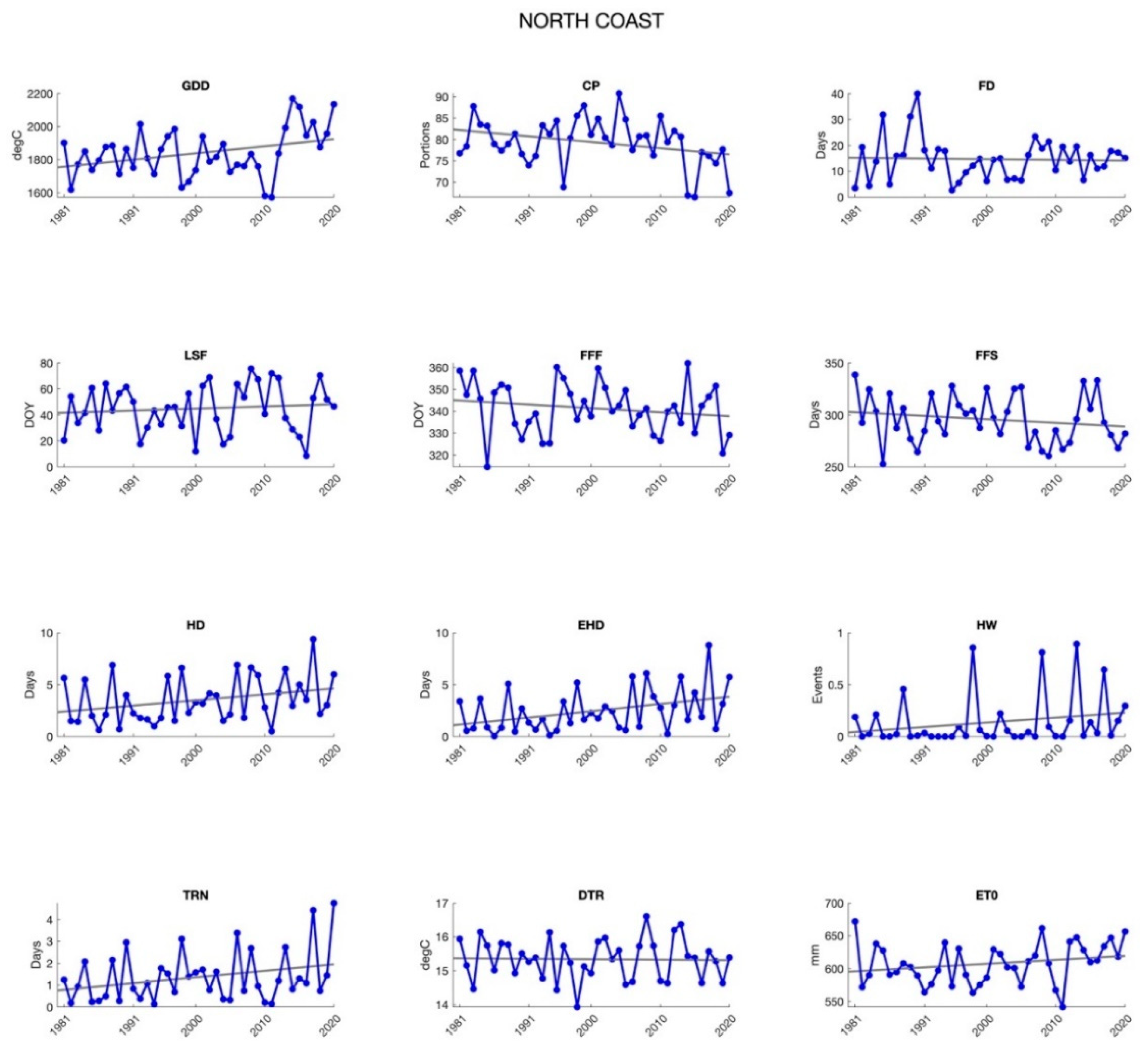
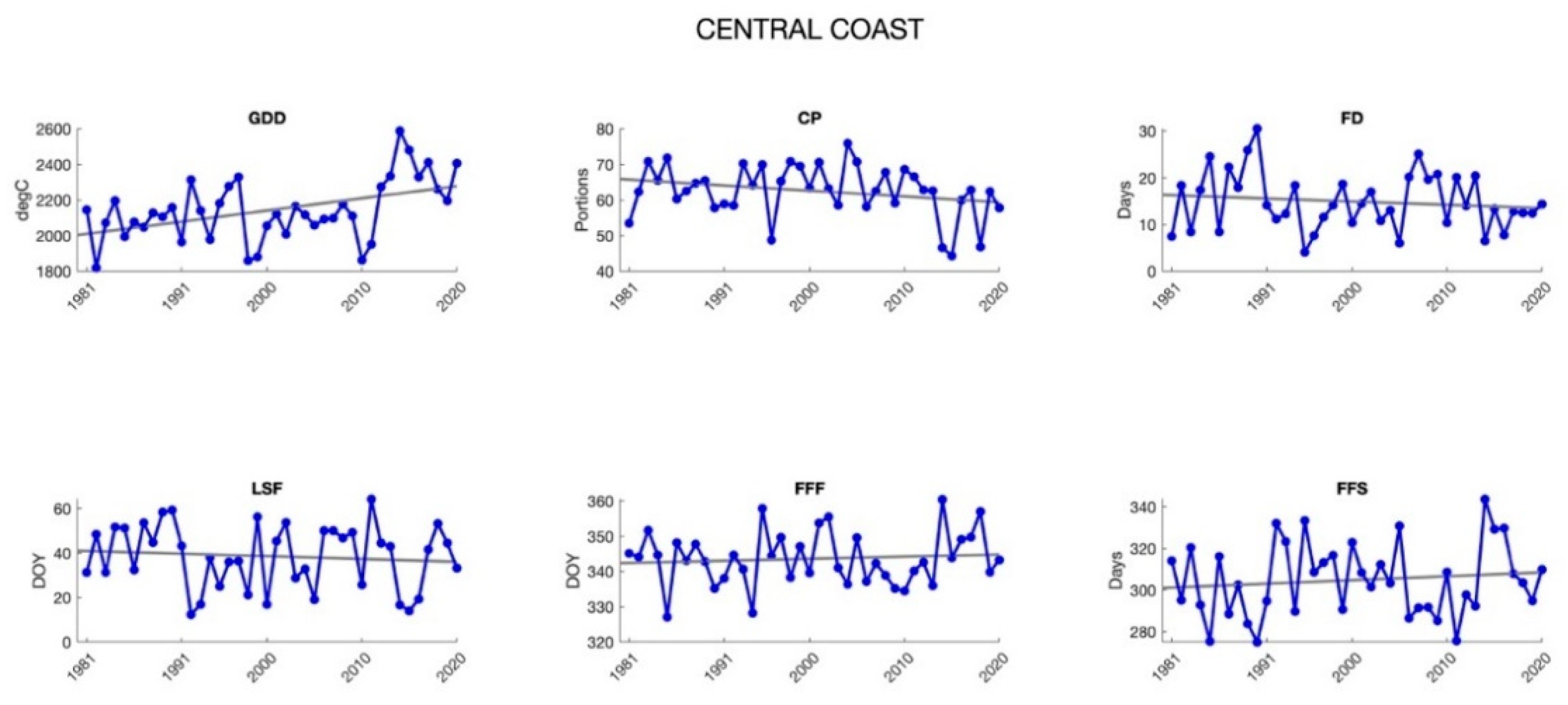
3.1.1. North and Central Coasts

The metrics showing the largest relative changes over the coast regions were those related to heat exposure, including daytime heatwaves (HW), heat days (HD), extreme heat days (EHD), and tropical nights (TRN). Though no metrics showed a significant difference between periods over the North Coast, average EHD showed a significant difference between periods over the Central Coast, increasing in the new normal period by 1.3 days. Growing degree days (GDD) also showed the largest relative increase (3.9%), equating to the second largest absolute increase (~77DD) over the Central Coast as compared to other regions. Positive trends in GDD and EHD were significant across both coast regions, and the Central Coast also showed significant positive trends in the number of HD, HW, and TRN. Given the considerable winegrape acreage across the coast regions, metrics such as EHD and HD heat are particularly important to monitor as heat exposure has known effects on winegrape berry development and chemistry, influencing traits including pigmentation, malic acid concentration, total soluble solids, berry size, and sugar content [41,61]. Likewise, increased TRN can similarly impact the berry chemistry (Gaiotti et al., 2018) and increase the pathogen susceptibility [39] in winegrapes, as well as lowering yields [40]. However, we note that while heat metrics showed the largest relative increase over the coast regions, the high percent changes can be attributed to their infrequent occurrence in these regions during the prior normal period.

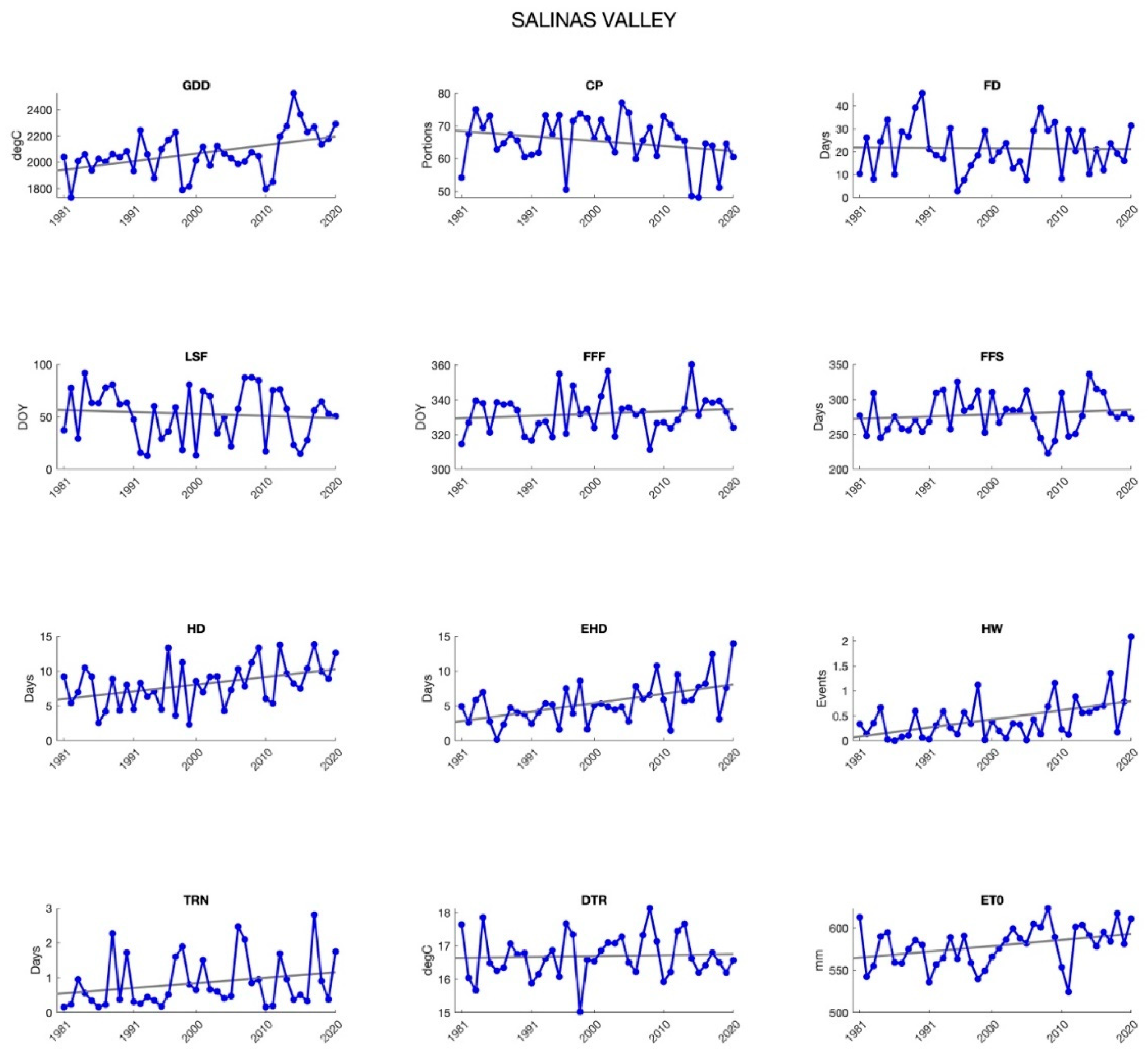
3.1.2. Salinas Valley

Over the Salinas Valley, the number of heatwave events (HW), average heat days (HD) and extreme heat days (EHD) all showed large relative increases during the new normal period (64.4%, 46.4%, and 40.8%, respectively), equating to an additional ~0.2 HW, ~1.2 HD and ~1.3 EHD during the new normal period, respectively. All three metrics showed significant 40-year trends, and the difference between periods was significant for EHD. The metrics with the most notable absolute change were the date of last spring freeze (LSF), the length of the frost-free season (FFS), and growing degree days (GDD). On average, LSF occurred 4.8 days earlier over the new normal period, combined with a first fall freeze (FFF) occurring 1.4 days later on average, the FFS lengthened by nearly one week. These changes align with previous work showing earlier LSF, later FFF, and longer FFS over California during the 20th and early 21st century [62]. The average GDD over the Salinas Valley increased by more than 75 degree days between the old and new normal periods, and this metric also showed a significant trend over the 40 years of study. For annual specialty crops, changes in LSF, FFS, and GDD have implications for planting and harvest dates (e.g., [36]), as well as pest pressure and the number of annual generations of pests [37]. As the top crops in the Salinas Valley are annual fruits and vegetables, shifts in planting and harvest dates are important considerations for crop and variety selection and farm management planning.

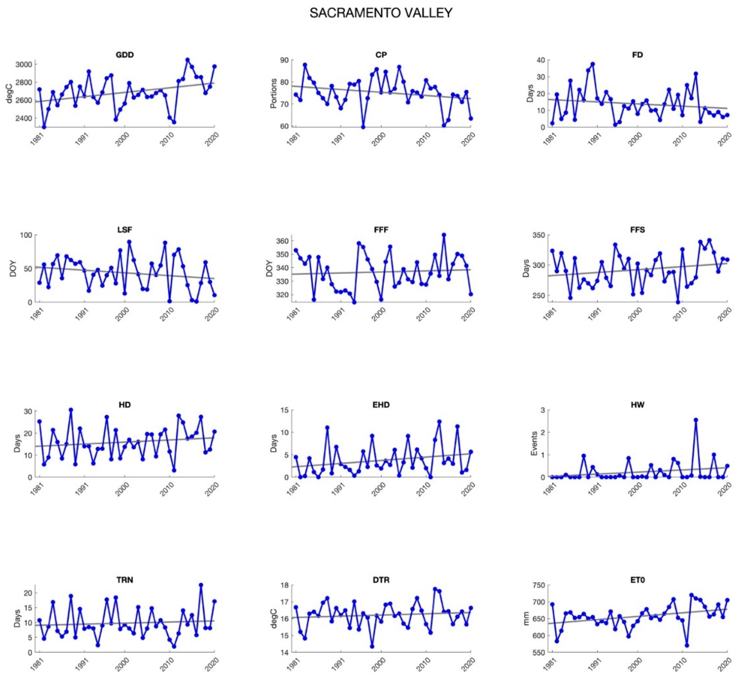
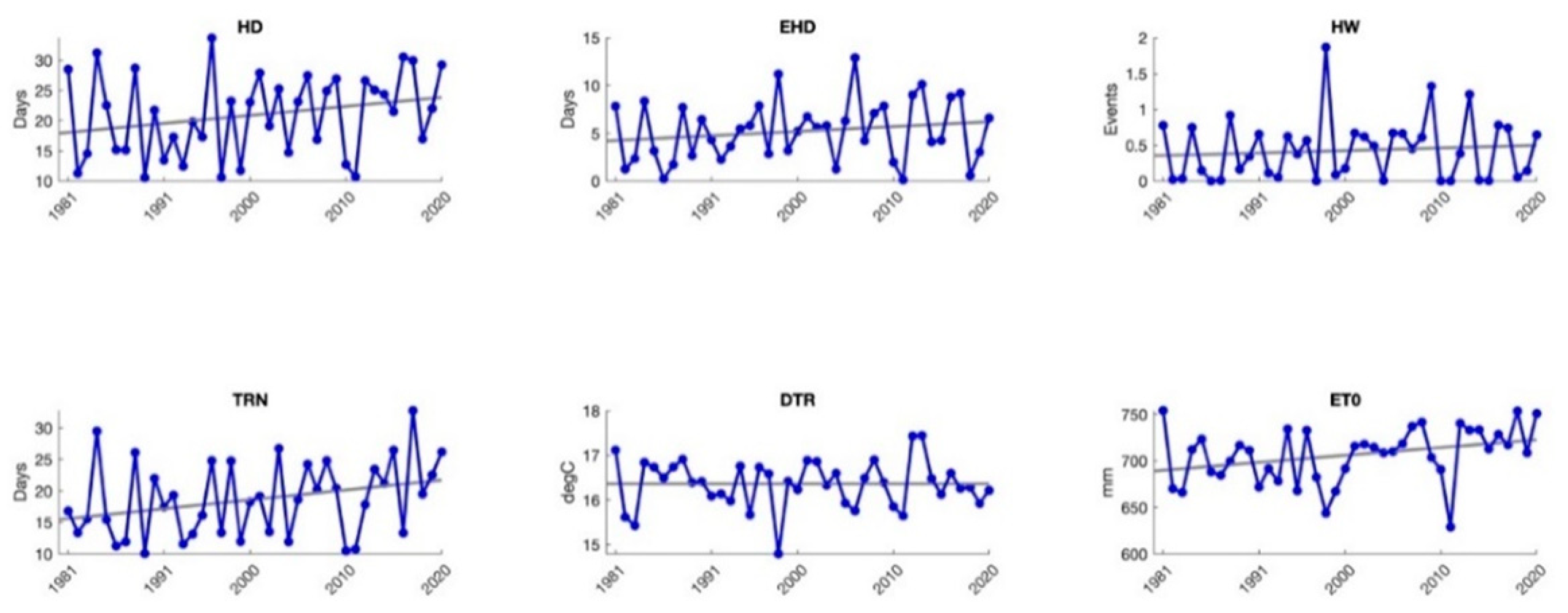
3.1.3. Sacramento and San Joaquin Valleys

Shifts in agroclimate metrics over the Sacramento and San Joaquin Valleys include an earlier last spring freeze (LSF) of ~3 (San Joaquin) and 5 (Sacramento) days, and a >5 day longer frost-free season (FFS). The results also showed a ~1–2 day reduction in frost days (FD), an increase in growing degree days (GDD) of 65 DD over the Sacramento Valley and 68.5 DD over the San Joaquin Valley, as well as a reduction in chill portions (CP) of nearly two portions for both regions. GDD showed a significant 40-year trend over both regions. The observed trends in LSF show an ~3-week advance in LSF and a ~7-day reduction in FD in the Sacramento Valley over the 1981–2020 period; the San Joaquin valley also showed an advance in LSF and a reduction in FD over the 40-year period, though to a lesser degree. The trends in LSF and FD across both valleys complement prior observations of warming springs and reduced frost days [63,64]. Likewise, the observed reduction in CP aligns with previous observations of reduced chill accumulation over corresponding [65] and longer [33,66] time periods. Specialty crops in these regions are highly sensitive to winter temperatures [67], and growers are already facing chill-related challenges (e.g., [68]). Moreover, warmer springs and increased GDD can lead to greater navel orangeworm pressure, an important pest for nut crops grown widely across these valleys [69]. Finally, during the 1991–2020 period, summer reference evapotranspiration (ETo) was ~6 mm (~0.2 in) and ~8.8 mm (~0.35 in) higher than the 1981–2010 period for the San Joaquin and Sacramento Valleys, respectively. Moreover, trend analyses show a significant ~40 mm increase in summer ETo during 1981–2020 in these regions. The increased ETo is consistent with warming and its role in increased vapor pressure deficit [70] and decreased Palmer Drought Severity Index (PDSI; [71]).

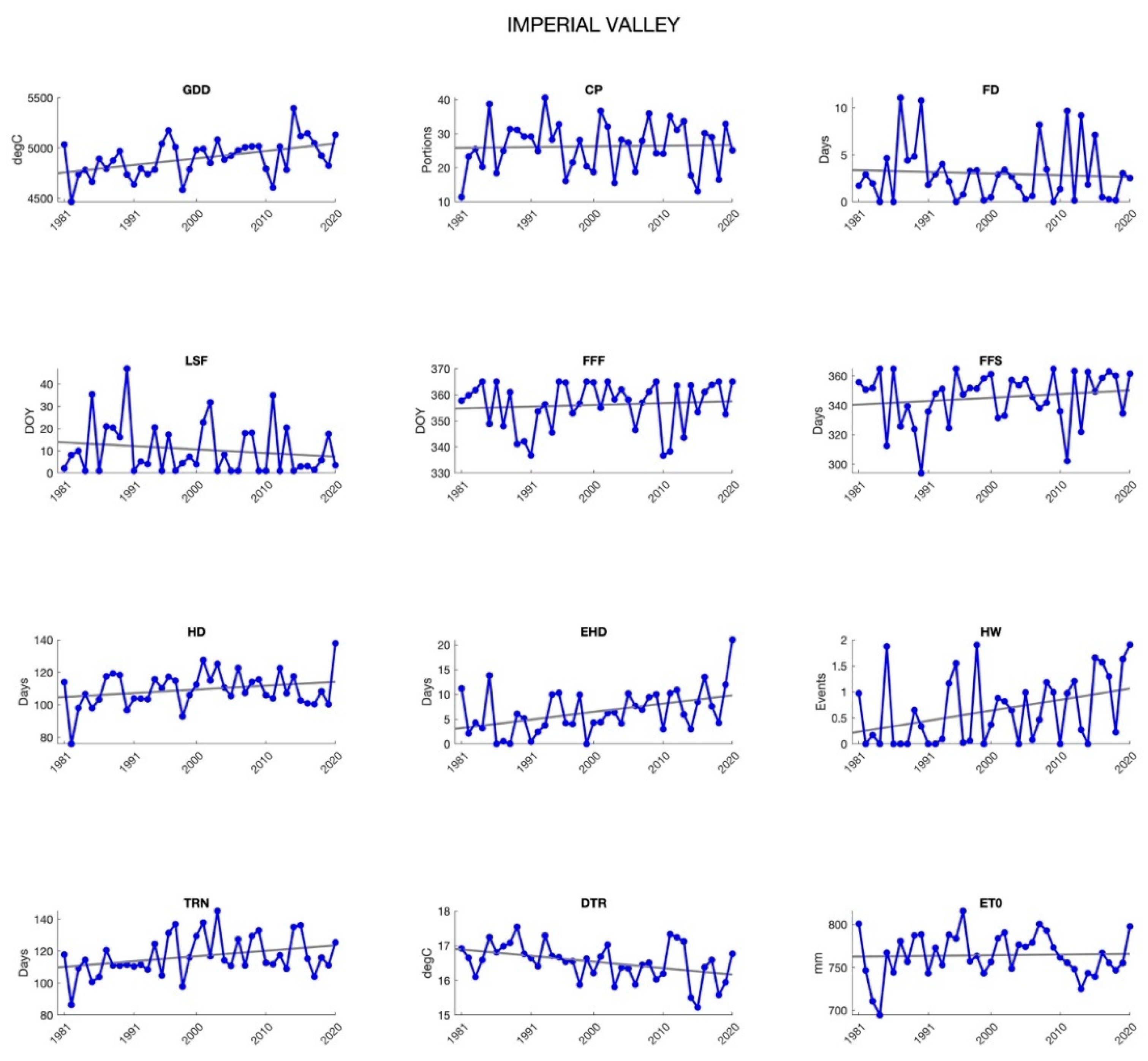
3.1.4. Coachella and Imperial Valleys

The Coachella and Imperial Valleys showed the largest changes in tropical nights (TRN) and diurnal temperature range (DTR) of all agricultural regions, with the TRN increasing by 6.4 nights (3.1 nights) in the Coachella (Imperial) Valley and DTR compressing by 0.2 °C (0.3 °C). The between-period differences for TRN and DTR were significant over the Coachella Valley, and the 40-year trends in these metrics were significant over both regions. Notably, we show an 11.7 and 26.6 day increase in TRN from 1981 to 2020 for the Imperial Valley and Coachella Valley, respectively. The negative trend in DTR is directionally consistent with global DTR patterns over the 20th century [72]. DTR changes are important for agricultural pest life-cycles as they have been shown to alter the pest phenology even in the absence of increased mean daily temperature [73]. In addition, heat days (HD) and extreme heat days (EHD) showed the greatest absolute changes over the Imperial Valley of any region, with EHD having a significant trend over the 1981–2020 period. For some specialty crops grown in these regions (e.g., table grapes, leafy greens, peppers, and pomegranates), increases in heat exposure are important for crop quality considerations as extreme heat can lead to sunburn damage and yield losses (e.g., [74,75]). Despite increases in heat metrics, we note that the Coachella and Imperial Valleys showed the least change in climatological summer reference evapotranspiration (ETo) between periods (+1.7 mm and −1.6 mm, respectively), and both valleys showed only a slight trend in summer ETo over the 40-year period. However, increased heat exposure can increase irrigation water use, and any increased irrigation (whether for heat damage mitigation or to meet increased crop water demand) may promote feedback between irrigation and TRN [76], contributing to DTR compression.

3.2. Adapting for the Future

Changes and trends in agroclimate metrics between normal periods provide context for the longer-term shifts stemming from ongoing climate change. Future climate projections of warmer temperatures across seasons and geographies suggest that the positive trends we showed in metrics such as growing degree days and the frost-free season and the complementary negative trends in chill portions and frost days will continue in coming decades—along with their attendant challenges. Climate change is also projected to increase the incidence of heat days, extreme heat days, and heatwaves across California [42,77] (also see [78]). Future warming trends are also projected to further shift harvest dates and alter the planting dates and/or geography of crop production. For example, [36] showed that the time between transplantation and harvest for processing tomatoes in the Central Valley may compress by as much as 3 weeks under projected mid-century climate conditions. Recent work by [43] indicated that for cool-season crops such as lettuce, warming trends will alter the timing of crop production, whereas for warm-season crops such as tomatoes, higher summer temperatures may reduce the suitability for cultivation by over as much as 66% of historic tomato-growing locations, thereby shifting the geography of crop cultivation. Future climate change is also projected to expand the pest range and increase pest pressure [37,69], and could severely reduce or eliminate the successful cultivation of some crops in the state (e.g., [33]). Within this context, adaptation approaches for sustaining specialty crop production must be considered. California producers already utilize a number of adaptive practices to contend with climate variability and climate stressors (e.g., selecting heat-tolerant or low-chill crop varieties [42] and using integrated pest management approaches [69]). Moreover, research efforts (e.g., [65]) and resource and tool development continue to provide advancements in support of the adaptive capacity of California producers. However, producers will still be challenged to adopt new adaptive management strategies. For example, in a future with increased evaporative demand [79], reduced surface-water availability from a more limited snowpack [80], and decreased groundwater availability due to declining reserves [81] and regulatory restrictions on pumping (e.g., reduced allocations stemming from the enactment of the Sustainable Groundwater Management Act [82]), approaches that can increase the amount of water available for irrigation will be warranted. Such approaches may include agricultural managed aquifer recharge (AgMAR), which could increase the resilience to drought and aridification and potentially return tens of millions of acre feet of water to California’s aquifers over the long term [83,84]. Similarly, triple-win practices such as the incorporation of soil amendments [85,86,87] that provide adaptive and mitigation benefits will be increasingly important as California’s agriculture is pushed to adapt to climate change, mitigate climate change, and remain economically viable.
Finally, as we consider adapting for the future, we note that while climate normals such as those presented here use a 30-year period, the significant trends identified in this work suggest that even the most recent normals (e.g., 1991–2020) may already be ill-suited to contextualizing current conditions. Though NCEI released supplementary products averaged over 15, 10, and 5 years to provide additional (and potentially more appropriate) measures of average contemporary climate, given non-stationary climate conditions, it is questionable to what degree backward-looking normals have utility for forward-looking decision-making [88,89]. In light of these considerations, successful agricultural adaptation will arguably require that those working in the decision support space understand the nature of climate normals, how their computation can alter their ‘meaning’, and how communication of this meaning can alter the action and outcome (e.g., [90]).

4. Conclusions

Here, we explored the changes and trends in climatological normals for a suite of agroclimate metrics between the previous normal period and the new normal period across seven key agricultural regions in California, highlighted the implications of these changes for specialty crop production, and placed these shifts in the context of future climate change and agricultural adaptation. Though most differences and trends were not statistically significant, the direction of change was generally in line with broader climate changes, the implications of which are for increasing difficulties for California’s agricultural sector and a growing need to adopt adaptive management strategies. However, in the absence of systematic and consistent analysis of agriculturally relevant metrics at standard timesteps, subtle shifts may be missed. Moreover, without careful communication around what is ‘normal’, there is the risk of misunderstanding around issues such as climate variability, anomalous weather events, and ‘extremes’ that often spur adaptive action. The establishment of a standardized list of agroclimate metrics that are assessed at the timestep of climate normals and compared against previous normal periods (as we present here for California specialty crops) can address these challenges and provide information in support of the much-needed efforts to bolster California agriculture’s adaptive capacity. Finally, we note that these methods can be applied in other agriculturally-important regions—both within the U.S.A. and globally—and suggest that agriculture-focused organizations consider undertaking future efforts to this end as the benefits of calculating agroclimate normals are worth the computational cost.

Author Contributions

Conceptualization, L.E.P., N.Z., J.T.A., S.M.O. and T.B.P.; methodology, L.E.P., N.Z., J.T.A., S.M.O. and T.B.P.; software, L.E.P., N.Z., J.T.A., S.M.O. and T.B.P.; validation, L.E.P., N.Z. and J.T.A.; formal analysis, N.Z. and L.E.P.; investigation, N.Z., L.E.P. and J.T.A.; resources, S.M.O., T.B.P. and J.T.A.; data curation, N.Z.; writing—original draft preparation, L.E.P.; writing—review and editing, L.E.P., J.T.A., S.M.O. and T.B.P.; visualization, L.E.P., N.Z. and J.T.A.; supervision, S.M.O. and T.B.P.; project administration, L.E.P.; funding acquisition, S.M.O. and T.B.P. All authors have read and agreed to the published version of the manuscript.

Funding

This work was supported in part through funds to the USDA California Climate Hub from the USDA Office of the Chief Economist award number OCE 60-2032-1-002, and from the USDA National Institute of Food and Agriculture award number 2021-68012-35914. Author Zhang was supported in part through funds from the University of California Office of the President, Multicampus Research Programs and Initiatives. Author Abatzoglou was supported in part through funds from USDA National Institute of Food and Agriculture award number 2021-69012-35916.

Data Availability Statement

Data used in this study can be found at https://www.climatologylab.org/gridmet.html.

Conflicts of Interest

The authors have no conflicts of interest to report.

Appendix A

Table A1. The formulae for growing degree days, chill portions, and reference evapotranspiration as given in the citations in Table 1.
Agroclimate MetricCalculation
Growing Degree Days (GDD)GDD is calculated following [28]:
GDD = { T x + T n 2     T b a s e ,     T x +   T n 2 > T b a s e   0 , T x +   T n 2   T b a s e
Where Tbase = 10 °C
Chill Accumulation (as Chill Portions, CP)Chill accumulation is calculated as chill portions (CP) [30] using hourly T calculated following [31]. Annual CP are accumulated 1st Nov–1st Mar [32].
[31] calculates hourly temperature for each day using daily maximum and minimum temperatures, and sunrise and sunset times. Hourly temperatures from sunrise to sunset are calculated as:
T ( t ) = ( T x T n )     sin [ π t D L + 4 ] + T x
Where T(t) is the temperature at time t after sunrise, Tx is the daily maximum temperature, Tn is the daily minimum temperature, and DL is the daylength in hours.
Hourly temperatures from sunset to sunrise are calculated as:
T = [ T s T n 24 D L ]       ln ( t )
Where T(t) is the temperature at time t > 1 h after sunset, Ts is the temperature at sunset based on the equation above, Tn is the minimum daily temperature, and DL is the daylength in hours.
The equations for calculating chill portions at time t (CPt) are:
x i = e s l p t e t m l t   T K t e t m l t T K 1 +   e s l p t e t m l t T k t e t m l t T K
x s = a 0 a 1   e e 1 e 0 T K
a k 1 = a 1   e ( e 1 T K )
i n t e r E   = x s ( x s i n t e r s )   e a k 1
i n t e r S   = { t = t 0   : 0 t > t 0 i n t e r E t 1 < 1 : i n t e r E t 1 t > t 0 i n t e r E t 1 1 : i n t e r E t 1 ( 1 x i t 1 )
d e l t = { t = t 0 : 0 t > t 0 i n t e r E < 1 : 0 t > t 0 i n t e r E 1 : x i     i n t e r E
C P t = { t = t 0 : d e l t t t 0 : d e l t + C P t 1
Where hourly temperature is in degrees Kelvin (TK), and the constants are:
slp = 1.6
tetmlt = 277
a0 = 139,500
a1 = 2.567 × 10¹⁸
e0 = 4153.5
e1 = 12,888.8
Reference Evapotranspiration (ETo)ETo is calculated following the FAO Penman–Monteith method [27]. We calculate summer (June–August) average ETo for each year 1981–2020 for our analysis. ETo units are mm.
The FAO Penman–Monteith formula for ETo is given in [27] as:
ETo = 0.408 ( R n G ) + γ 900 T + 273 u 2 ( e s e a ) + γ ( 1 + 0.34 u 2 )
where
ETo is the reference evapotranspiration in units mm day−1
Rn is the net radiation at the crop surface in units MJ m−2 day−1
G is the soil heat flux density in units MJ m−2 day−1
T is the mean daily air temperature at 2 m height in units °C
u2 is the wind speed at 2 m height in units m second−1
es is the mean daily saturation vapor pressure in units kPa
ea is the mean daily vapor pressure in units kPa
∆ is the slope vapor pressure curve in units kPa °C−1
γ is the psychrometric constant in units kPa °C−1
Figure A1. Annual agroclimate metrics averaged over the North Coast region with linear trendline. Metrics are shown as: row 1: growing degree days (GDD), chill portions (CP), frost days (FD); row 2: last spring freeze (LSF), first fall freeze (FFF), frost-free season (FFS); row 3: heat days (HD), extreme heat days (EHD), heatwaves (HW); row 4: tropical nights (TRN), diurnal temperature range (DTR), summer reference evapotranspiration (ETo). GDD and EHD have statistically significant trends over the 40-year period.
Agronomy 12 00205 g0a1
Figure A2. Annual agroclimate metrics averaged over the Central Coast region with linear trendline. Metrics are shown as: row 1: growing degree days (GDD), chill portions (CP), frost days (FD); row 2: last spring freeze (LSF), first fall freeze (FFF), frost-free season (FFS); row 3: heat days (HD), extreme heat days (EHD), heatwaves (HW); row 4: tropical nights (TRN), diurnal temperature range (DTR), summer reference evapotranspiration (ETo). GDD, HD, EHD, HW, and TRN have statistically significant trends over the 40-year period.
Agronomy 12 00205 g0a2aAgronomy 12 00205 g0a2b
Figure A3. Annual agroclimate metrics averaged over the Salinas Valley region with linear trendline. Metrics are shown as: row 1: growing degree days (GDD), chill portions (CP), frost days (FD); row 2: last spring freeze (LSF), first fall freeze (FFF), frost-free season (FFS); row 3: heat days (HD), extreme heat days (EHD), heatwaves (HW); row 4: tropical nights (TRN), diurnal temperature range (DTR), summer reference evapotranspiration (ETo). GDD, HD, EHD, HW, and ETo have statistically significant trends over the 40-year period.
Agronomy 12 00205 g0a3
Figure A4. Annual agroclimate metrics averaged over the Sacramento Valley region with linear trendline. Metrics are shown as: row 1: growing degree days (GDD), chill portions (CP), frost days (FD); row 2: last spring freeze (LSF), first fall freeze (FFF), frost-free season (FFS); row 3: heat days (HD), extreme heat days (EHD), heatwaves (HW); row 4: tropical nights (TRN), diurnal temperature range (DTR), summer reference evapotranspiration (ETo). GDD and ETo have statistically significant trends over the 40-year period.
Agronomy 12 00205 g0a4
Figure A5. Annual agroclimate metrics averaged over the San Joaquin Valley region with linear trendline. Metrics are shown as: row 1: growing degree days (GDD), chill portions (CP), frost days (FD); row 2: last spring freeze (LSF), first fall freeze (FFF), frost-free season (FFS); row 3: heat days (HD), extreme heat days (EHD), heatwaves (HW); row 4: tropical nights (TRN), diurnal temperature range (DTR), summer reference evapotranspiration (ETo). GDD and ETo have statistically significant trends over the 40-year period.
Agronomy 12 00205 g0a5aAgronomy 12 00205 g0a5b
Figure A6. Annual agroclimate metrics averaged over the Coachella Valley region with linear trendline. Metrics are shown as: row 1: growing degree days (GDD), chill portions (CP), frost days (FD); row 2: last spring freeze (LSF), first fall freeze (FFF), frost-free season (FFS); row 3: heat days (HD), extreme heat days (EHD), heatwaves (HW); row 4: tropical nights (TRN), diurnal temperature range (DTR), summer reference evapotranspiration (ETo). GDD, TRN, and DTR have statistically significant trends over the 40-year period.
Agronomy 12 00205 g0a6
Figure A7. Annual agroclimate metrics averaged over the Imperial Valley region with linear trendline. Metrics are shown as: row 1: growing degree days (GDD), chill portions (CP), frost days (FD); row 2: last spring freeze (LSF), first fall freeze (FFF), frost-free season (FFS); row 3: heat days (HD), extreme heat days (EHD), heatwaves (HW); row 4: tropical nights (TRN), diurnal temperature range (DTR), summer reference evapotranspiration (ETo). GDD, TRN, EHD, HW, and DTR have statistically significant trends over the 40-year period.
Agronomy 12 00205 g0a7

References

  1. Lamb, P.J.; Changnon, S.A. On the “Best” Temperature and Precipitation Normals: The Illinois Situation. J. Appl. Meteorol. Climatol. 1981, 20, 1383–1390. [Google Scholar] [CrossRef] [Green Version]
  2. Trewin, B. The Role of Climatological Normals in a Changing Climate; Baddour, O., Kontongomde, H., Eds.; WMO-TD No. 1377; World Meteorological Organization: Geneva, Switzerland, 2007; Available online: https://library.wmo.int/doc_num.php?explnum_id=4546 (accessed on 24 November 2021).
  3. World Meteorological Organization. WMO Guidelines on the Calculation of Climate Normal; World Meteorological Organization: Geneva, Switzerland, 2017. [Google Scholar]
  4. Fountain, H.; Kao, J. There’s a New Definition of “Normal” for Weather. (Original Work Published 2021). Available online: https://www.nytimes.com/interactive/2021/05/12/climate/climate-change-weather-noaa.html (accessed on 12 May 2021).
  5. Henson, B.; Samenow, J. NOAA Unveils New U.S. Climate “Normals” That Are Warmer than Ever. Washington Post. (Original Work Published 2021). Available online: https://www.washingtonpost.com/weather/2021/05/04/noaa-new-climate-normals/ (accessed on 4 May 2021).
  6. Ludden, J. Your Weather Forecast Update: Warmer Climate Will Be the New “Normal”. (Original Work Published 2021). Available online: https://www.npr.org/2021/04/07/983224262/your-weather-forecast-update-warmer-climate-will-be-the-new-normal (accessed on 7 April 2021).
  7. Arguez, A.; Durre, I.; Applequist, S.; Vose, R.S.; Squires, M.F.; Yin, X.; Heim, R.R.; Owen, T.W. NOAA’s 1981–2010 U.S. Climate Normals: An Overview. Bull. Am. Meteorol. Soc. 2012, 93, 1687–1697. [Google Scholar] [CrossRef]
  8. Katz, R.W.; Brown, B.G. Extreme events in a changing climate: Variability is more important than averages. Clim. Chang. 1992, 21, 289–302. [Google Scholar] [CrossRef]
  9. Román-Palacios, C.; Wiens, J.J. Recent responses to climate change reveal the drivers of species extinction and survival. Proc. Natl. Acad. Sci. USA 2020, 117, 4211–4217. [Google Scholar] [CrossRef]
  10. Woodward, F.I.; Lomas, M.R.; Kelly, C.K. Global climate and the distribution of plant biomes. Philos. Trans. R. Soc. B Biol. Sci. 2004, 359, 1465–1476. [Google Scholar] [CrossRef] [PubMed] [Green Version]
  11. California Department of Food and Agriculture. California Agricultural Statistics Review, 2019–2020. 2020; (Original work published 2020). Available online: https://www.cdfa.ca.gov/Statistics/PDFs/2020_Ag_Stats_Review.pdf (accessed on 24 November 2021).
  12. Macaulay, L.; Butsic, V. Ownership characteristics and crop selection in California cropland. Calif. Agric. 2017, 71, 221–230. [Google Scholar] [CrossRef]
  13. Lobell, D.; Cahill, K.N.; Field, C.B. Historical effects of temperature and precipitation on California crop yields. Clim. Chang. 2007, 81, 187–203. [Google Scholar] [CrossRef]
  14. Ortiz-Bobea, A.; Wang, H.; Carrillo, C.M.; Ault, T.R. Unpacking the climatic drivers of US agricultural yields. Environ. Res. Lett. 2019, 14, 064003. [Google Scholar] [CrossRef]
  15. Lobell, D.B.; Field, C.B.; Cahill, K.N.; Bonfils, C. Impacts of future climate change on California perennial crop yields: Model projections with climate and crop uncertainties. Agric. For. Meteorol. 2006, 141, 208–218. [Google Scholar] [CrossRef] [Green Version]
  16. Crimmins, T.M. Applying the USA National Phenology Network’s Growing Degree Day Maps in Making Management Decisions. J. Ext. 2018, 56, 2. [Google Scholar]
  17. Jagannathan, K.A. Ready-to-Use?—Bridging the Climate Science-Usability Gap for Adaptation; UC Berkeley: Berkeley, CA, USA, 2019; Available online: https://escholarship.org/uc/item/3q56j15f (accessed on 24 November 2021).
  18. Matthews, K.; Rivington, M.; Buchan, K.; Miller, D.; Bellocchi, G. Characterising the agro-meteorological implications of climate change scenarios for land management stakeholders. Clim. Res. 2008, 37, 59–75. [Google Scholar] [CrossRef]
  19. Zhu, X.; Troy, T.J. Agriculturally Relevant Climate Extremes and Their Trends in the World’s Major Growing Regions. Earth’s Futur. 2018, 6, 656–672. [Google Scholar] [CrossRef]
  20. Fernández-Long, M.E.; Müller, G.V.; Beltrán-Przekurat, A.; Scarpati, O.E. Long-term and recent changes in temperature-based agroclimatic indices in Argentina. Int. J. Clim. 2013, 33, 1673–1686. [Google Scholar] [CrossRef]
  21. Lalić, B.; Eitzinger, J.; Thaler, S.; Vučetić, V.; Nejedlik, P.; Eckersten, H.; Jaćimović, G.; Nikolić-Djorić, E. Can Agrometeorological Indices of Adverse Weather Conditions Help to Improve Yield Prediction by Crop Models? Atmosphere 2014, 5, 1020–1041. [Google Scholar] [CrossRef] [Green Version]
  22. Eitzinger, J.; Thaler, S.; Orlandini, S.; Nejedlik, P.; Kazandjiev, V.; Sivertsen, T.H.; Mihailovic, D. Applications of agroclimatic indices and process oriented crop simulation models in European agriculture. Idojaras 2009, 113, 1–12. [Google Scholar]
  23. Hatfield, J.L.; Antle, J.; Garrett, K.A.; Izaurralde, R.; Mader, T.; Marshall, E.; Nearing, M.; Robertson, G.P.; Ziska, L. Indicators of climate change in agricultural systems. Clim. Chang. 2020, 163, 1719–1732. [Google Scholar] [CrossRef] [Green Version]
  24. Tubiello, F.N.; Rosenzweig, C. Developing climate change impact metrics for agriculture. Integr. Assess. 2008, 8. Available online: http://116.203.146.222:8080/index.php/iaj/article/viewArticle/276 (accessed on 24 November 2021).
  25. Walsh, M.; Backlund, P.; Buja, L.; DeGaetano, A.; Melnick, R.; Prokopy, L.; Takle, E.; Todey, D.; Ziska, L. Climate Indicators for Agriculture; USDA Technical Bulletin 1953: Washington, DC, USA, 2020; pp. 1–70. [Google Scholar] [CrossRef]
  26. Johnson, R.; Cody, B.A. California Agricultural Production and Irrigated Water Use. 2015. Available online: https://nationalaglawcenter.org/wp-content/uploads/assets/crs/R44093.pdf (accessed on 23 September 2021).
  27. Allen, R.G.; Pereira, L.S.; Raes, D.; Smith, M. Crop evapotranspiration-Guidelines for computing crop water requirements-FAO Irrigation and drainage paper 56. Fao Rome 1998, 300, D05109. [Google Scholar]
  28. McMaster, G.S.; Wilhelm, W.W. Growing degree-days: One equation, two interpretations. Agric. For. Meteorol. 1997, 87, 291–300. [Google Scholar] [CrossRef] [Green Version]
  29. Jones, G.V.; Duff, A.A.; Hall, A. Spatial analysis of climate in winegrape growing regions in the western United States. Am. J. Enol. Vitic. 2010, 61, 313–326. Available online: https://www.ajevonline.org/content/61/3/313.short (accessed on 24 November 2021).
  30. Luedeling, E.; Brown, P.H. A global analysis of the comparability of winter chill models for fruit and nut trees. Int. J. Biometeorol. 2010, 55, 411–421. [Google Scholar] [CrossRef] [Green Version]
  31. Linvill, D.E. Calculating Chilling Hours and Chill Units from Daily Maximum and Minimum Temperature Observations. HortScience 1990, 25, 14–16. [Google Scholar] [CrossRef] [Green Version]
  32. Pope, K.S.; Dose, V.; Da Silva, D.; Brown, P.; DeJong, T.M. Nut crop yield records show that budbreak-based chilling requirements may not reflect yield decline chill thresholds. Int. J. Biometeorol. 2015, 59, 707–715. [Google Scholar] [CrossRef]
  33. Luedeling, E.; Zhang, M.; Girvetz, E.H. Climatic Changes Lead to Declining Winter Chill for Fruit and Nut Trees in California during 1950–2099. PLoS ONE 2009, 4, e6166. [Google Scholar] [CrossRef]
  34. Reyes, J.J.; Elias, E. Spatio-temporal variation of crop loss in the United States from 2001 to 2016. Environ. Res. Lett. 2019, 14, 074017. [Google Scholar] [CrossRef]
  35. Parker, L.; Pathak, T.; Ostoja, S. Climate change reduces frost exposure for high-value California orchard crops. Sci. Total Environ. 2021, 762, 143971. [Google Scholar] [CrossRef] [PubMed]
  36. Pathak, T.B.; Stoddard, C.S. Climate change effects on the processing tomato growing season in California using growing degree day model. Model. Earth Syst. Environ. 2018, 4, 765–775. [Google Scholar] [CrossRef]
  37. Trumble, J.T.; Butler, C.D. Climate change will exacerbate California’s insect pest problems. Calif. Agric. 2008, 63, 73–78. [Google Scholar] [CrossRef]
  38. Gaiotti, F.; Pastore, C.; Filippetti, I.; Lovat, L.; Belfiore, N.; Tomasi, D. Low night temperature at veraison enhances the accumulation of anthocyanins in Corvina grapes (Vitis vinifera L.). Sci. Rep. 2018, 8, 8719. [Google Scholar] [CrossRef] [PubMed] [Green Version]
  39. Aoki, Y.; Usujima, A.; Suzuki, S. High night temperature promotes downy mildew in grapevine via attenuating plant defence response and enhancing early Plasmopara viticola infection. Plant. Prot. Sci. 2020, 57, 21–30. [Google Scholar] [CrossRef]
  40. Cahill, K.N.; Lobell, D.B.; Field, C.B.; Bonfils, C.; Hayhoe, K. Modeling climate change impacts on wine grape yields and quality in California. Semin. Réchauffement Clim. Quels Impacts Probables Sur Les Vign. 2007, 28–30. Available online: https://www.researchgate.net/publication/237227560 (accessed on 24 November 2021).
  41. Greer, D.H.; Weston, C. Heat stress affects flowering, berry growth, sugar accumulation and photosynthesis of Vitis vinifera cv. Semillon grapevines grown in a controlled environment. Funct. Plant. Biol. 2010, 37, 206–214. [Google Scholar] [CrossRef]
  42. Parker, L.E.; McElrone, A.J.; Ostoja, S.M.; Forrestel, E.J. Extreme heat effects on perennial crops and strategies for sustaining future production. Plant. Sci. 2020, 295, 110397. [Google Scholar] [CrossRef] [PubMed]
  43. Marklein, A.; Elias, E.; Nico, P.; Steenwerth, K. Projected temperature increases may require shifts in the growing season of cool-season crops and the growing locations of warm-season crops. Sci. Total Environ. 2020, 746, 140918. [Google Scholar] [CrossRef]
  44. Gershunov, A.; Cayan, D.R.; Iacobellis, S.F. The Great 2006 Heat Wave over California and Nevada: Signal of an Increasing Trend. J. Clim. 2009, 22, 6181–6203. [Google Scholar] [CrossRef] [Green Version]
  45. Sheridan, S.C.; Lee, C. Temporal Trends in Absolute and Relative Extreme Temperature Events across North America. J. Geophys. Res. Atmos. 2018, 123, 11–889. [Google Scholar] [CrossRef]
  46. Martínez-Lüscher, J.; Chen, C.C.L.; Brillante, L.; Kurtural, S.K. Mitigating Heat Wave and Exposure Damage to “Cabernet Sauvignon” Wine Grape with Partial Shading under Two Irrigation Amounts. Front. Plant. Sci. 2020, 11, 1760. [Google Scholar] [CrossRef] [PubMed]
  47. Pathak, T.B.; Maskey, M.L.; Dahlberg, J.A.; Kearns, F.; Bali, K.M.; Zaccaria, D. Climate Change Trends and Impacts on California Agriculture: A Detailed Review. Agronomy 2018, 8, 25. [Google Scholar] [CrossRef] [Green Version]
  48. Cohen, S.D.; Tarara, J.M.; Kennedy, J.A. Diurnal Temperature Range Compression Hastens Berry Development and Modifies Flavonoid Partitioning in Grapes. Am. J. Enol. Vitic. 2011, 63, 112–120. [Google Scholar] [CrossRef]
  49. Cohen, S.D.; Tarara, J.M.; Gambetta, G.A.; Matthews, M.A.; Kennedy, J.A. Impact of diurnal temperature variation on grape berry development, proanthocyanidin accumulation, and the expression of flavonoid pathway genes. J. Exp. Bot. 2012, 63, 2655–2665. [Google Scholar] [CrossRef] [Green Version]
  50. Jones, G.V.; Reid, R.; Vilks, A. Climate, grapes, and wine: Structure and suitability in a variable and changing climate. In The Geography of Wine: Regions, Terroir and Techniques; Springer Press: Amsterdam, The Netherlands, 2012; pp. 109–133. [Google Scholar] [CrossRef]
  51. Zhang, J.; Guan, K.; Peng, B.; Jiang, C.; Zhou, W.; Yang, Y.; Pan, M.; Franz, T.E.; Heeren, D.M.; Rudnick, D.R.; et al. Challenges and opportunities in precision irrigation decision-support systems for center pivots. Environ. Res. Lett. 2021, 16, 053003. [Google Scholar] [CrossRef]
  52. Alston, J.M.; Lapsley, J.T.; Sambucci, O. Grape and wine production in California. California Agriculture: Dimensions and Issues. Giannini Found. Agric. Econ. 2018, 8, 1–28. [Google Scholar]
  53. Yang, L.; Jin, S.; Danielson, P.; Homer, C.; Gass, L.; Bender, S.M.; Case, A.; Costello, C.; Dewitz, J.; Fry, J.; et al. A new generation of the United States National Land Cover Database: Requirements, research priorities, design, and implementation strategies. ISPRS J. Photogramm. Remote. Sens. 2018, 146, 108–123. [Google Scholar] [CrossRef]
  54. Abatzoglou, J.T. Development of gridded surface meteorological data for ecological applications and modelling. Int. J. Clim. 2013, 33, 121–131. [Google Scholar] [CrossRef]
  55. Soule, P.T. A Comparison of 30-yr Climatic Temperature Normals for the Southeastern United States. Southeast. Geogr. 2005, 45, 16–24. [Google Scholar] [CrossRef]
  56. Shea, D. The Climate Data Guide: Trend Analysis. In National Center for Atmospheric Research Staff; NCAR Climate Data Guide; National Center for Atmospheric Research: Boulder, CO, USA, 2014; Available online: https://climatedataguide.ucar.edu/climate-data-tools-and-analysis/trend-analysis (accessed on 24 November 2021).
  57. California Department of Food and Agriculture. 2019 California Almond Acreage Report. 2020; (Original work published 2020). Available online: https://www.nass.usda.gov/Statistics_by_State/California/Publications/Specialty_and_Other_Releases/Almond/Acreage/202004almac.pdf (accessed on 24 November 2021).
  58. United States Department of Agriculture National Agricultural Statistics Service (USDA-NASS). 2019 California Walnut Acreage Report. 2020; (Original work published 2020). Available online: https://www.nass.usda.gov/Statistics_by_State/California/Publications/Specialty_and_Other_Releases/Walnut/Acreage/2020walac_revised.pdf (accessed on 24 November 2021).
  59. Volpe, R.; Green, R.; Helen, D.; Howitt, R. Recent Trends in the California Wine Grape Industry. Calif. Agric. 2010, 64, 42–46. [Google Scholar] [CrossRef]
  60. California Department of Food and Agriculture. California Grape Acreage Report 2019 Crop. 2020. Available online: https://www.nass.usda.gov/Statistics_by_State/California/Publications/Specialty_and_Other_Releases/Grapes/Acreage/2020/202004gabtb00.pdf (accessed on 24 November 2021).
  61. Buttrose, M.S.; Hale, C.R. Effect of temperature on the composition of’Cabernet Sauvignon’berries. Am. J. Enol. Vitic. 1971, 22, 71–75. Available online: https://www.ajevonline.org/content/22/2/71.short?casa_token=65zS9BAqSyYAAAAA:h6uL_j7CMjoIFq6oV4FKYiwRQ269DAbD-60kETncsnUU35lv3jsCRCS3yVZ20XJ_w1w8oYQ (accessed on 24 November 2021).
  62. Kukal, M.S.; Irmak, S. U.S. Agro-Climate in 20th Century: Growing Degree Days, First and Last Frost, Growing Season Length, and Impacts on Crop Yields. Sci. Rep. 2018, 8, 6977. [Google Scholar] [CrossRef]
  63. Cordero, E.C.; Kessomkiat, W.; Abatzoglou, J.; Mauget, S.A. The identification of distinct patterns in California temperature trends. Clim. Chang. 2011, 108, 357–382. [Google Scholar] [CrossRef]
  64. Easterling, D.R. Recent changes in frost days and the frost-free season in the united states. Bull. Am. Meteorol. Soc. 2002, 83, 1327–1332. [Google Scholar] [CrossRef]
  65. Zhang, N.; Pathak, T.B.; Parker, L.E.; Ostoja, S.M. Impacts of large-scale teleconnection indices on chill accumulation for specialty crops in California. Sci. Total. Environ. 2021, 791, 148025. [Google Scholar] [CrossRef]
  66. Baldocchi, D.; Wong, S. Accumulated Winter Chill is Decreasing in the Fruit Growing Regions of California. Clim. Chang. 2008, 87, 153–166. [Google Scholar] [CrossRef]
  67. Kerr, A.; DiAlesandro, J.; Steenwerth, K.; Lopez-Brody, N.; Elias, E. Vulnerability of California specialty crops to projected mid-century temperature changes. Clim. Chang. 2017, 148, 419–436. [Google Scholar] [CrossRef]
  68. Sommer, L. As Warm Winters Mess with Nut Trees’ Sex Lives, Farmers Help Them “Netflix and Chill.” NPR. Available online: https://www.npr.org/sections/thesalt/2020/02/17/805688641/warm-winters-threaten-nut-trees-can-science-help-them-chill-out (accessed on 17 February 2020).
  69. Pathak, T.B.; Maskey, M.L.; Rijal, J.P. Impact of climate change on navel orangeworm, a major pest of tree nuts in California. Sci. Total. Environ. 2021, 755, 142657. [Google Scholar] [CrossRef]
  70. Ficklin, D.L.; Novick, K.A. Historic and projected changes in vapor pressure deficit suggest a continental-scale drying of the United States atmosphere. J. Geophys. Res. Atmos. 2017, 122, 2061–2079. [Google Scholar] [CrossRef]
  71. He, M.; Gautam, M. Variability and Trends in Precipitation, Temperature and Drought Indices in the State of California. Hydrology 2016, 3, 14. [Google Scholar] [CrossRef] [Green Version]
  72. Easterling, D.R.; Horton, B.; Jones, P.D.; Peterson, T.C.; Karl, T.R.; Parker, D.E.; Salinger, M.J.; Razuvayev, V.; Plummer, N.; Jamason, P.; et al. Maximum and minimum temperature trends for the globe. Science 1997, 277, 364–367. [Google Scholar] [CrossRef] [Green Version]
  73. Chen, S.; Fleischer, S.J.; Saunders, M.C.; Thomas, M.B. The Influence of Diurnal Temperature Variation on Degree-Day Accumulation and Insect Life History. PLoS ONE 2015, 10, e0120772. [Google Scholar] [CrossRef] [PubMed]
  74. Gambetta, J.M.; Holzapfel, B.P.; Stoll, M.; Friedel, M. Sunburn in Grapes: A Review. Front. Plant. Sci. 2021, 11, 2123. [Google Scholar] [CrossRef]
  75. Hartz, T.; Cantwell, M.; LeStrange, M.; Smith, R.; Aguiar, J.; Daugovish, O. Bell Pepper Production in California; University of California Agriculture and Natural Resources (UC ANR): Davis, CA, USA, 2008. [Google Scholar]
  76. Kanamaru, H.; Kanamitsu, M. Model Diagnosis of Nighttime Minimum Temperature Warming during Summer due to Irrigation in the California Central Valley. J. Hydrometeorol. 2008, 9, 1061–1072. [Google Scholar] [CrossRef]
  77. Gershunov, A.; Guirguis, K. California heat waves in the present and future. Geophys. Res. Lett. 2012, 39. [Google Scholar] [CrossRef] [Green Version]
  78. Cal-Adapt. Extreme Heat Days & Warm Nights. Cal-Adapt; UC Berkeley, California Energy Commission, California Strategic Growth Council. Available online: https://cal-adapt.org/tools/extreme-heat/ (accessed on 18 May 2021).
  79. McEvoy, D.J.; Pierce, D.W.; Kalansky, J.F.; Cayan, D.R.; Abatzoglou, J.T. Projected Changes in Reference Evapotranspiration in California and Nevada: Implications for Drought and Wildland Fire Danger. Earth’s Futur. 2020, 8, e2020EF001736. [Google Scholar] [CrossRef]
  80. Cayan, D.R.; Maurer, E.; Dettinger, M.D.; Tyree, M.; Hayhoe, K. Climate change scenarios for the California region. Clim. Chang. 2008, 87, 21–42. [Google Scholar] [CrossRef]
  81. Massoud, E.C.; Purdy, A.J.; Miro, M.E.; Famiglietti, J. Projecting groundwater storage changes in California’s Central Valley. Sci. Rep. 2018, 8, 12917. [Google Scholar] [CrossRef] [PubMed]
  82. Babbitt, C.; Dooley, D.; Hall, M.; Moss, R.; Orth, D.; Sawyers, G. Groundwater Pumping Allocations under California’s Sustainable Groundwater Management Act. Considerations for Groundwater Sustainability Agencies. Environmental Defense Fund and New Current Water and Land LLC. 2018. Available online: https://www.edf.org/sites/default/files/documents/edf_california_sgma_allocations.pdf (accessed on 24 November 2021).
  83. Dahlke, H.E.; LaHue, G.T.; Mautner, M.R.L.; Murphy, N.P.; Patterson, N.K.; Waterhouse, H.; Yang, F.; Foglia, L. Chapter Eight—Managed Aquifer Recharge as a Tool to Enhance Sustainable Groundwater Management in California: Examples from Field and Modeling Studies. In Advances in Chemical Pollution, Environmental Management and Protection; Friesen, J., Rodríguez-Sinobas, L., Eds.; Elsevier: Amsterdam, The Netherlands, 2018; Volume 3, pp. 215–275. [Google Scholar]
  84. Scanlon, B.R.; Reedy, R.C.; Faunt, C.C. Enhancing Drought Resilience with Conjunctive Use and Managed Aquifer Recharge in California and Arizona. The Environmentalist. 2016. Available online: https://0-iopscience-iop-org.brum.beds.ac.uk/article/10.1088/1748-9326/11/3/035013/meta (accessed on 24 November 2021).
  85. Abel, S.; Peters, A.; Trinks, S.; Schonsky, H.; Facklam, M.; Wessolek, G. Impact of biochar and hydrochar addition on water retention and water repellency of sandy soil. Geoderma 2013, 202–203, 183–191. [Google Scholar] [CrossRef]
  86. Jahanzad, E.; Holtz, B.A.; Zuber, C.A.; Doll, D.; Brewer, K.M.; Hogan, S.; Gaudin, A.C.M. Orchard recycling improves climate change adaptation and mitigation potential of almond production systems. PLoS ONE 2020, 15, e0229588. [Google Scholar] [CrossRef]
  87. Martínez-Blanco, J.; Lazcano, C.; Christensen, T.H.; Muñoz, P.; Rieradevall, J.; Møller, J.; Antón, A.; Boldrin, A. Compost benefits for agriculture evaluated by life cycle assessment. A review. Agron. Sustain. Dev. 2013, 33, 721–732. [Google Scholar] [CrossRef] [Green Version]
  88. Arguez, A.; Vose, R.S. The Definition of the Standard WMO Climate Normal: The Key to Deriving Alternative Climate Normals. Bull. Am. Meteorol. Soc. 2011, 92, 699–704. [Google Scholar] [CrossRef]
  89. Livezey, R.E.; Vinnikov, K.Y.; Timofeyeva, M.M.; Tinker, R.; Dool, H.M.V.D. Estimation and Extrapolation of Climate Normals and Climatic Trends. J. Appl. Meteorol. Clim. 2007, 46, 1759–1776. [Google Scholar] [CrossRef] [Green Version]
  90. Hulme, M.; Dessai, S.; Lorenzoni, I.; Nelson, D.R. Unstable climates: Exploring the statistical and social constructions of “normal” climate. Geoforum 2009, 40, 197–206. [Google Scholar] [CrossRef]
Figure 1. Fruits, nuts, and vegetables are largely grown across 7 geographic regions within California. While agricultural valleys are responsible for most production, the north and central coast regions are known for winegrape production. Basemap data are from the 2016 NLCD [53].
Agronomy 12 00205 g001
Figure 2. Changes in 12 agroclimate metrics between the previous (1981–2010) and current (1991–2020) normal periods. Agricultural regions are outlined in grey. Metrics are shown as: row 1: growing degree days (GDD), chill portions (CP), frost days (FD); row 2: last spring freeze (LSF), first fall freeze (FFF), frost-free season (FFS); row 3: heat days (HD), extreme heat days (EHD), heatwaves (HW); row 4: tropical nights (TRN), diurnal temperature range (DTR), summer reference evapotranspiration (ETo).
Agronomy 12 00205 g002
Figure 3. Trends in 12 agroclimate metrics over the 40-year (1981–2020) period averaged over crop locations in each agricultural region. Trends are per year. Metrics in red are statistically significant. Metrics are shown as: row 1: growing degree days (GDD), chill portions (CP), frost days (FD); row 2: last spring freeze (LSF), first fall freeze (FFF), frost-free season (FFS); row 3: heat days (HD), extreme heat days (EHD), heatwaves (HW); row 4: tropical nights (TRN), diurnal temperature range (DTR), summer reference evapotranspiration (ETo).
Agronomy 12 00205 g003
Table 1. The 12 agroclimate metrics selected for this analysis, how they are calculated or defined, and their relevance to specialty crop production. Formulae for GDD, CP, and ETo are provided in Table A1.
Agroclimate MetricCalculationRelevance to Specialty Crop Production
Growing Degree Days (GDD)GDD is calculated following [28] using Tbase = 10 °C.
  • Use in crop and pest phenology models
  • Can inform crop or cultivar growing location [29]
Chill Accumulation (as Chill Portions, CP)Chill accumulation is calculated as chill portions (CP) [30] using hourly T calculated following [31]. Annual CP are accumulated 1st Nov–1st Mar [32].
  • Sufficient chill is necessary for fruit development and good crop yield [33]
Frost Days (FD)FD are the number of days per year with minimum temperatures (Tn) ≤ 0 °C.
  • Frost damages have significant economic consequences [34,35]
  • Frost risk is a top grower concern [17]
Last Spring Freeze (LSF)The LSF is defined as the last day of the calendar year prior to 30 June with a Tn ≤ 0 °C.
  • Consideration for early-blooming and frost-sensitive perennials
  • Governs transplant dates for annual crops [36]
  • Earlier LSF can increase pest pressure [37]
First Fall Freeze(FFF)The FFF is defined as the first day of the calendar year commencing 1 July with Tn ≤ 0 °C.
  • Important for late-maturing crops that can suffer fruit damage from a fall freeze [35]
  • Can serve as a guide for planting dates of late-season annual crops
Freeze-Free Season (FFS)The FFS is calculated as the difference between the LSF and FFF (FFF [minus] LSF).
  • Can inform the geography of crop cultivation
  • Longer FFS can increase pest pressure [37]
Tropical Nights (TRN)TRN are calculated as the number of nights per year with Tn > 20 °C.
  • Can reduce fruit set in tomatoes [25]
  • Impacts winegrape berry chemistry [38], pathogen susceptibility [39], and yield [40]
  • May decrease yield of table grapes [13]
Hot Days (HD)The number of days per year with Tx > 38 °C [41,42].
  • Can negatively affect plant development and crop yield
  • Impacts are dependent on HD timing and crop heat tolerance
Extreme Heat Days (EHD)EHD are the number of days per year with Tx >98th percentile of summer (June-August) Tx for the 1981–2010 period [42].
  • EHD percentile threshold allows local heat impacts to be explored. For example, heat intolerant crops (e.g., broccoli, lettuce [43]) may be impacted by exposure to temperatures below the HD threshold.
Heatwaves (HW)HW events are defined as 3 + consecutive days [44,45] with Tx > 98th percentile of 1981–2010 summer Tx (as in EHD).
  • Impacts on crop yield and crop quality in winegrapes [46]
  • Impacts farmworker productivity and decreases occupational safety [47]
Diurnal Temperature Range (DTR)DTR is the difference between daily Tx and Tn.
We calculate DTR over 1 March to 1 November.
  • Reduced amplitude can alter winegrape berry chemistry [48,49], though effects can vary by cultivar [50]
Reference Evapotranspiration (ETo)ETo is calculated following the FAO Penman–Monteith method [27]. We calculate summer (June-August) average ETo for each year 1981–2020 for our analysis. ETo units are mm.
  • Commonly used in irrigation models and decision support systems [51]
  • Considered a proxy for plant water demand.
Table 2. Five high-value example crops, the percent of U.S. production occurring in California, the total value of each crop based on crop receipts for California producers, the total acreage in the state, the top three California counties by acreage, based on the CDL.
Crop% U.S. Production in CaliforniaValue ($1000 USD)Total California Area (Hectares)
Almonds>99% [11]6,094,440 [11]360,642 (hectares bearing and non-bearing; [57])
Walnuts>99% [11]1,286,410 [11]178,062 (hectares bearing and non-bearing; [58])
Winegrapes>90% [59]3,806,320 [11]193,052 (hectares bearing and non-bearing; [60])
Lettuces52% [11]1,824,435 [11]76,364 (hectares harvested; [11])
Tomatoes73% [11]1,174,395 [11]100,241 (hectares harvested; [11])
Table 3. Agroclimate metrics over crop locations in each agriculture region for 1981–2010, 1991–2020, the absolute and relative difference between 1981–2010 and 1991–2020, and the 40-year trend over the 1981–2020 period. Underlined values indicate statistical significance in difference or trend.
Agro-Climate MetricNorth Coast
1981–20101991–2020(1991–2020)–(1981–2010)(1991–2020)–(1981–2010) (%)40-year (1981–2020) Trend
GDD (°C)1927.91986.558.63.0198.2
CP (portions)80.078.0−2.0−2.5−5.6
FD (days)16.014.6−1.3−6.70.9
LSF (day of year)47.446.4−1.13.55.5
FFF (day of year)340.2339.3−0.9−0.2−8.7
FFS (days)292.3292.40.10.4−14.7
TRN (days)1.51.80.334.01.2
HD (days)3.64.00.438.02.2
EHD (days)2.52.90.535.92.1
HW (events)0.10.2048.20
DTR (°C)15.915.90−0.3−0.1
ETo (mm)625.1629.94.80.736.4
Central Coast
1981–20101991–2020(1991–2020)–(1981–2010)(1991–2020)–(1981–2010) (%)40-year (1981–2020) Trend
GDD (°C)2017.02094.177.13.9244.7
CP (portions)66.364.2−2.1−3.2−4.8
FD (days)14.112.8−1.3−13.3−1.1
LSF (day of yr)36.334−2.3−1.9−1.8
FFF (day of yr)343.5344.20.80.2−0.7
FFS (days)306.93103.01.52.2
TRN (days)1.51.90.443.11
HD (days)3.23.80.656.12.6
EHD (days)3.64.91.347.24.7
HW (events)0.20.40.270.90.4
DTR (°C)14.914.9−0.1−0.5−0.4
ETo (mm)555.6558.62.90.526.3
Salinas Valley
1981–20101991–2020(1991–2020)–(1981–2010)(1991–2020)–(1981–2010) (%)40-year (1981–2020) Trend
GDD (°C)2013.42088.575.13.8230.4
CP (portions)67.265.4−1.8−2.7−4.7
FD (days)22.721.5−1.2−2.80.6
LSF (day of yr)54.749.9−4.8−2.3−10.3
FFF (day of yr)330.1331.51.40.42.9
FFS (days)274.8281.06.22.78.4
TRN (days)0.60.70.122.40.2
HD (days)8.09.31.246.45.2
EHD (days)4.55.81.340.84.9
HW (events)0.30.50.264.40.6
DTR (°C)17.017.00.00.10.1
ETo (mm)576.7580.640.731.7
Sacramento Valley
1981–20101991–2020(1991–2020)–(1981–2010)(1991–2020)–(1981–2010) (%)40-year (1981–2020) Trend
GDD (°C)2642.32707.365.02.5221.3
CP (portions)76.474.5−1.9−2.5−5.3
FD (days)14.212.4−1.8−12.3−7.3
LSF (day of yr)45.139.9−5.2−11.4−22.4
FFF (day of yr)335.6336.81.30.41.3
FFS (days)289.7296.26.52.321.9
TRN (days)8.28.20.0−2.30.2
HD (days)15.115.80.75.25.2
EHD (days)3.44.00.620.92.5
HW (events)0.20.30.166.20.0
DTR (°C)16.416.50.00.20.0
ETo (mm)650.6659.48.81.437.4
San Joaquin Valley
1981–20101991–2020(1991–2020)–(1981–2010)(1991–2020)–(1981–2010) (%)40-year (1981–2020) Trend
GDD (°C)2878.82947.368.52.4237.4
CP (portions)73.371.5−1.8−2.5−5.7
FD (days)15.614.4−1.2−8.4−0.6
LSF (day of yr)41.237.9−3.3−7.2−10.4
FFF (day of yr)334.6336.41.80.56.0
FFS (days)292.6297.75.11.812.4
TRN (days)18.119.51.45.47.5
HD (days)21.823.21.46.18.0
EHD (days)5.76.10.59.62.7
HW (events)0.50.50.09.50.1
DTR (°C)16.516.50.00.0−0.2
ETo (mm)702.7708.76.00.840.5
Coachella Valley
1981–20101991–2020(1991–2020)–(1981–2010)(1991–2020)–(1981–2010) (%)40-year (1981–2020) Trend
GDD (°C)4720.44820.8100.42.1415.4
CP (portions)30.430.1−0.4−1.20.6
FD (days)6.05.5−0.5−8.6−1.3
LSF (day of yr)17.813.9−3.9−22.7−13.2
FFF (day of yr)348.4348.60.203.2
FFS (days)330.2334.34.11.321.7
TRN (days)106112.46.46.026.6
HD (days)111.9113.51.61.42.7
EHD (days)11.012.31.312.05.2
HW (events)1.31.50.213.30.2
DTR (°C)17.617.3−0.3−1.9−1.6
ETo (mm)826.7828.41.70.24.2
Imperial Valley
1981–20101991–2020(1991–2020)–(1981–2010)(1991–2020)–(1981–2010) (%)40-year (1981–2020) Trend
GDD (°C)4848.2491364.71.3292.8
CP (portions)26.526.90.31.30.7
FD (days)3.22.9−0.2−8.2−1.0
LSF (day of yr)11.99.7−2.2−19.4−0.2
FFF (day of yr)354.8355.60.80.22.9
FFS (days)342.7345.73.10.910.3
TRN (days)115.3118.43.12.711.7
HD (days)109.4111.11.71.54.4
EHD (days)5.26.81.631.97.1
HW (events)0.50.70.248.10.6
DTR (°C)16.716.5−0.2−1.0−0.8
ETo (mm)759.7758.1−1.6−0.2−5.4
The underline indicates statistical significance.
Publisher’s Note: MDPI stays neutral with regard to jurisdictional claims in published maps and institutional affiliations.

