1. Introduction
The agriculture industry plays a significant role in the economies of many countries. For this reason, the technological advancements in the agricultural industry are considered to be a vital contributor to the economy, as well as to sustainable development. The implementation of smart monitoring and automatic condition sensing systems in agricultural fields enable farmers to effectively monitor their land and take necessary actions to maintain productivity. Several new technologies and approaches [
1,
2] have been studied and implemented to promote continuous improvement in the agriculture sector. Computer vision-based systems [
2] for precision agriculture, hyper-spectral imaging [
3], and disease/productivity prediction [
4] are some examples. AirSurf, an automated and open-source analytic platform that combines computer vision techniques with deep learning to measure yield-related phenotypes from ultra-large aerial imagery, is presented in [
5]. Artificial Intelligence (AI)-based systems are used for the analysis and prediction of the five most produced grains in the world: maize, rice, wheat, soybean, and barley. A systematic review for AI applications in precision agriculture is presented in [
6].
Pakistan is an agricultural country, with the majority of the population associated with the agricultural industry directly or indirectly [
7]. Despite advancements in the agricultural sector and evolution of the concept of precision agriculture [
4], Pakistani farmers still lack access to modern technological advancements in the field and are forced to use conventional and traditional mechanisms for farming. In this paper, we have designed and implemented a Smart Irrigation System (SIS) [
8] and deployed it in different agricultural fields in Sindh and other parts of the country. The SIS is a Wireless Sensor Network (WSN) [
9], which collects information on temperature, soil moisture and humidity from a particular field and passes this information back to a central server station, which calculates the water required in a particular field and passes this information back to the farmer’s smart phone. The farmer then irrigates the crops as communicated by the application. This allows the farmer to save water resources while increasing the crop yield.
One of the major flaws in the current SIS system and most of the WSNs deployed around the world is the sudden failure of physical nodes deployed along with the WSNs. It is sometimes impossible to assess whether the physical nodes are passing on the correct sensor values or are malfunctioning over the course of time. The only way to identify malfunctioning physical nodes is through manual inspection, which is a tedious and cumbersome job. The malfunctioning sensor node also has drastic effects on any real-time system. Providing incorrect values to the farmer from the SIS system will have a very negative impact on the overall reliability and public perception of the system.
A study related to the current work is presented in [
10], which focuses on three vital parameters, i.e., the speedy and precise prediction of the network lifetime, internode distance and power level. Since these three constraints are closely associated with each other, by fixing the two parameters, one can predict the optimal value of the third parameter with high accuracy. Moreover, the more tedious and complicated task is to design a WSN (i.e., determining network parameters) whilst employing a heuristic algorithm for the neural network.
Another research study [
11] proposed a novel architecture based on a Long Short-Term Memory (LSTM) network. It uses an appropriate training function and introduces a target generation to find suitable ways to explain and deal with the complications related to RUL (Remaining Useful Life) [
12] estimations for physical systems. The different sensors, which uninterruptedly record diverse indicators about a working asset such as vibration intensity or applied pressure, gather data. The suggested network uses a bidirectional sequence processing methodology in a sequential fashion, bidirectional handshaking LSTM [
11], to continuously monitor the sequential data. Instead of partially processing units or sequences, it passes the final states from forward processing LSTM units to backward processing units up to the time of predictions, to ensure the immediate availability of predictions. The aforementioned research study also proposed that RUL training does not require the hypothesis related to the deterioration of function, as it is based on the calculation of sensor reading to determine the health of the current system.
Neural networks are used in image processing [
3], saliency detection [
13], biomedical image analysis [
14], drug design [
15] and weather forecasting applications [
16]. The use of neural networks (NN) in environment monitoring for the creation of datasets of atmospheric parameters as well as for weather forecasting is also increasing day by day. Researchers have trained deep neural networks for weather prediction accompanied with the complexity of climate model. With the advancement in computational speed and power, the availability of massive datasets, and complex deep architectures, consisting of millions of parameters, deep learning is becoming the state of the art in many fields, including agriculture [
17].
This study tries to solve this problem by designing a neural network, referred as a neural sensor, complementing a physical sensor. This research also endeavors to provide, with initial feasibility, a study that utilizes a neural network mimicking a physical sensor node. Using such a model may also increase the reliability and efficiency of the current water resource management system, SIS, while reducing the dependency on physical sensors to effectively facilitate farmers in managing the productivity of their agricultural fields.
The main contributions of this research study are:
The development of an LSTM-based smart system that provides readings for irrigation based on the predictive analysis of temperature, soil moisture and humidity.
The continuous validation of the developed smart system using both physical and neural sensor readings to avoid malfunctions.
A comprehensive comparative forecasting of temperature, humidity and moisture.
The rest of this paper is organized as follows: In
Section 2, the design methodology and data collection are presented, and in
Section 3, the results are discussed. Finally,
Section 4 concludes the paper with future prospects.
2. Materials and Methods
2.1. Design Methodology
A sequential model is a linear stack of layers which enables building of the model layer by layer, where each layer poses one input and one output tensor. A linear sequential model [
18,
19] is used as the development methodology for the neural sensor system. The proposed model is sequential in nature and consists of blocks to process input data and feedback. The complete SIS system data flow is shown in
Figure 1. It illustrates diverse stages and events of this model, which depicts the implementation of a neural network to mimic the behavior of the physical sensor node, deployed in the agricultural field. Neural networks are universally employed as predictive models [
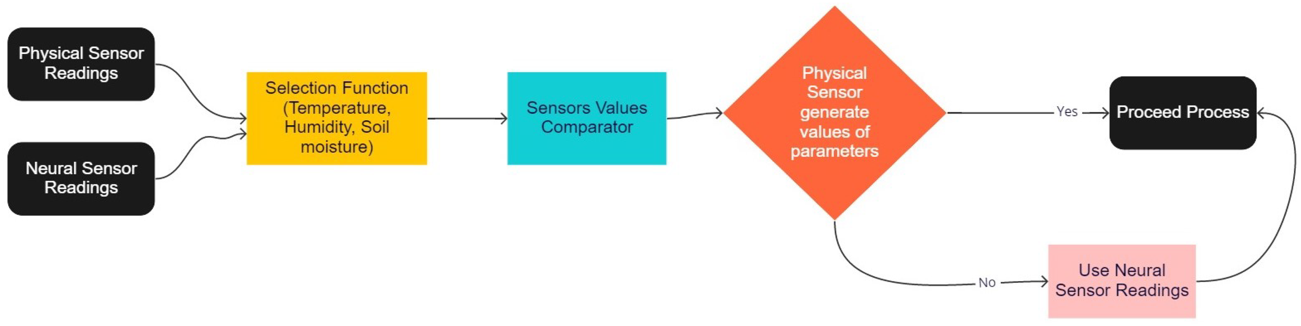
20]. In the proposed model, the neural network is trained in the supervised mode using actual data values acquired in the previous year by the SIS system deployed in the field. In supervised learning, the actual labels are also fed to the network during training. The data values mainly include temperature and humidity readings. The trained neural network will then be used to predict sensor data in the test mode. Since, there is a very little support available in the existing literature regarding the role of neural networks mimicking the behavior of a physical sensor node, the proposed module is referred to as a neural sensor. The flowchart of the complete system is shown in
Figure 1, which also illustrates how the proposed system operates.
2.2. Data Collection
This section emphasizes the data gathering and how the raw data were preprocessed by using different methods and techniques to obtain clean and observable data. The resulting data is used in the training of the proposed neural sensor model. Data processing is solely the alteration of raw data to extract meaningful information through a process. For the neural sensor, we used the data of physical sensors embedded in the agricultural field of lemons near Ghadap, Sindh, Pakistan.
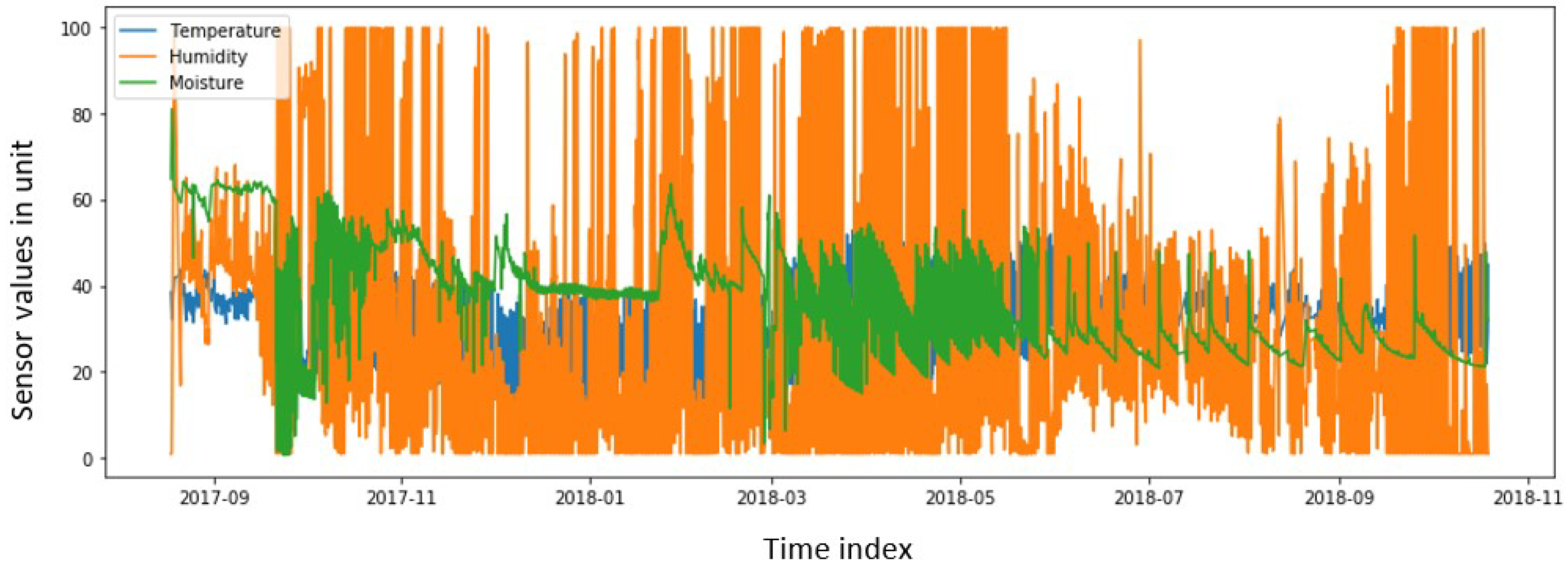
Data preprocessing consists of: importing data values, concatenating and sorting them, resampling the data, handling missing values and finally downsampling these values. The targeted variables in the dataset are temperature, humidity and soil moisture. The targeted variables plot is represented in
Figure 2, where the orange-colored graph shows the value of humidity against the date-time variable and blue-colored plot represents the temperature, while green represents the soil moisture readings of the physical sensor against a particular date-time variable. The plot shown in
Figure 2 consists of the values transmitted from the physical sensor of SIS fitted in the lemon crop field. Since index will not be a part of the prediction variable, the date components were extracted from it to highlight seasonality and time components.
The data values acquired from the field include temperature, humidity and the soil moisture values. The temperature value is relayed from a temperature sensor LM35 which is a precision integrated circuit (IC) temperature device. LM35 can operate accurately between temperature ranges of −50 degrees centigrade to 150 degrees centigrade, which is a sufficient range for the local temperatures in Pakistan. The humidity values are taken from the humidity sensor DHT-22. A customized in-house sensor has been designed to calculate the values of soil moisture in the agricultural field. Soil moisture works by passing a current between the two probes inserted closely in the soil and then measuring the strength of the output signal at the controller side. A comparator integrated circuit, LM 393, has been used to adjust the sensitivity of the soil moisture sensor. The data from the temperature, humidity and soil moisture sensors are passed to the controller, which transfers these values instantaneously to the cloud. The controller is tuned to transfer sensor values on an hourly basis to the main decision support system via the cloud.
2.3. Neural Sensor Modeling
A popular machine learning model used for data processing is a neural network (NN). A neural network is a set of algorithms that attempts to recognize the underlying relationships in a set of data using a method that is similar to how the human brain works. The architecture of an NN is inspired by the functional and structural aspects of a biological brain. A neuron receives inputs with adjustable weights along the incoming edges. In the most predictive model, the sigmoid or Relu activation function is frequently used as the activation function to model the non-linearity in the data [
21].
Recurrent Neural Networks (RNNs) [
22] are a robust type of neural network for processing sequence-dependent data as they handle variable length sequences and avoid the need for fixed-sized time windows. These are densely connected NNs with feedback loops to connect the hidden neurons across time. A state vector in the hidden units maintains the memory of all the previous elements of the sequence. Due to this internal memory, RNNs can learn the long-term dependencies across many time steps and generalize across input sequences rather than individual patterns. It is well suited for time-series analysis, forecasting, and many other areas of natural language processing [
23]. It enables precise future predictions based on the patterns of time series data.
A precise Recurrent Neural Network (RNN) architecture is demonstrated in
Figure 3, which is extended into a deep neural network to illustrate how a state is constructed with time. It takes an existing sequence element at time step t and the hidden state from the preceding time step at −1. Now, the hidden state (memory) updated to and the network output is determined. “U” is the weight matrix that maps the input to the hidden layer and “W” is the weight matrix for the recurrent transition among one hidden state to the next. The hidden layer is propagated to the output layer through the weight matrix “V”. Hence, the recent output is reliant on all the prior inputs (for
t ≤
t). Mathematically, it can be expressed as:
where
is the current state,
is the input, and
is the previous state. After that, the tanh activation function is applied.
where
is the weight matrix multiplied by the hidden state and
is the hidden matrix multiplied to the input sequence. Since, our data is sequential in nature, such a model is well suited to our problem.
LSTM networks are a specific RNN architecture that can maintain long-term dependencies. The core idea behind this architecture is a memory cell, which maintains the temporal state of the network over several time steps (over 1000), and non-linear analog gating units, which controls the information flow by selectively storing and deleting information in this cell. Initially, the basic LSTM components are the input gate, forget gate, output gate and hidden layer, i.e., the Constant Error Carousel (CEC).
The output gate controls what information needs to be released from the CEC and thus ensures that other units are not disturbed by the stored information. This architecture, however, led to instability in the network in the presence of a continuous input stream without any marked start and end points, as it did not reset the cell contents after finishing the processing of a sequence or before it started a new one. To deal with this issue, forget gates are used, which enable the LSTM cell to reset or forget the cell’s memory at appropriate times.
A typical LSTM architecture with forget gates and peephole connections, with LSTM RNNs, is shown in
Figure 3. The training of the network takes a shorter time and is of high accuracy compared to conventional RNNs. It prevents the error from back-propagating through time and makes it feasible for tasks with high complexity and temporal extent to learn over multiple time steps, thereby allowing the model to predict future data points based on long-term context dependencies without any vanishing gradient problem.
2.4. Training of the Neural Network
This section deals with the training of a neural sensor with the help of a recurrent neural network (LSTM). Since our data is sequential in nature with long-term dependencies, we decided to choose the Long Short-Term Memory (LSTM) architecture. Before applying the modeling technique, shift steps should be identified. Shift steps define how many steps into the future one wants to predict with each input to the network. It shifts the data backwards by the number of steps, and as one wants to predict into the future, the input and output dimensions remain the same. In the neural sensor, the shift steps number twenty-four for the input of each date, and it will generate twenty-four records of the predicted values of temperature, humidity and soil moisture on the hour against each date. These shifts have created an empty space in the tail of the target dataset equal to the number of shift steps. A sample dataset is shown in
Table 1.
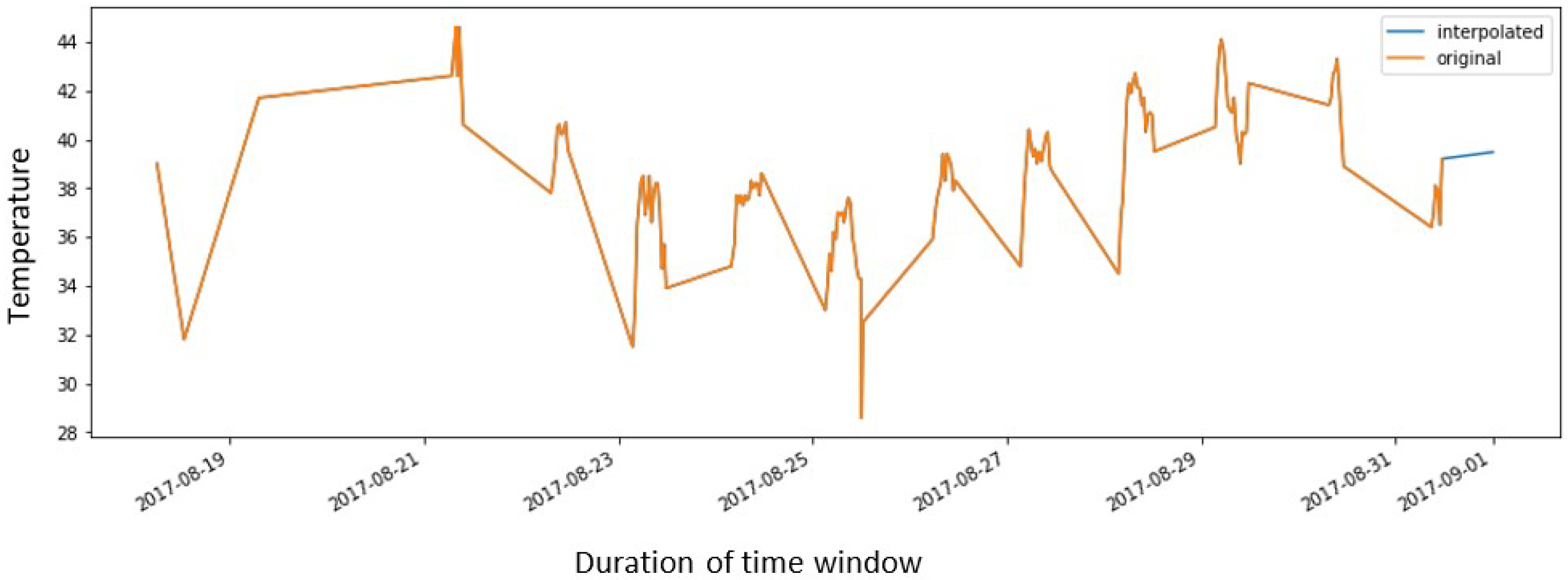
The bottom half from both the original and target datasets will be truncated, which correspond to the empty space. The number of rows remains the same, and we save them in x and y data where x corresponds to the input port of the neural net and y corresponds to the output port. Note that the output y data is ahead of the input x data in terms of number of shift steps. Interpolation was used to handle the missing values, as shown in
Figure 4.
To train the neural network, the dataset was splitted into a training dataset and testing dataset. The physical sensor readings for temperature, humidity and soil moisture were used as an input, and the neural network output was the future predicted values for temperature, humidity and soil moisture. We chose the common criteria of 80–20% split. In total,
of the data were used for training and
of the data were used for testing purposes. This allowed us to obtain a reasonable number of samples to train our models, and out of 10,223 records, 8178 records were assigned for training and 2045 were allocated for testing. We did not prepare the validation sets. Validations sets are used for hyper-parameter tuning [
24]. We tuned our parameters during the training phase and they also performed well during the testing phase. Root mean square propagation was used as an optimizer with a learning rate of 0.01. We divided the data into twenty batches.
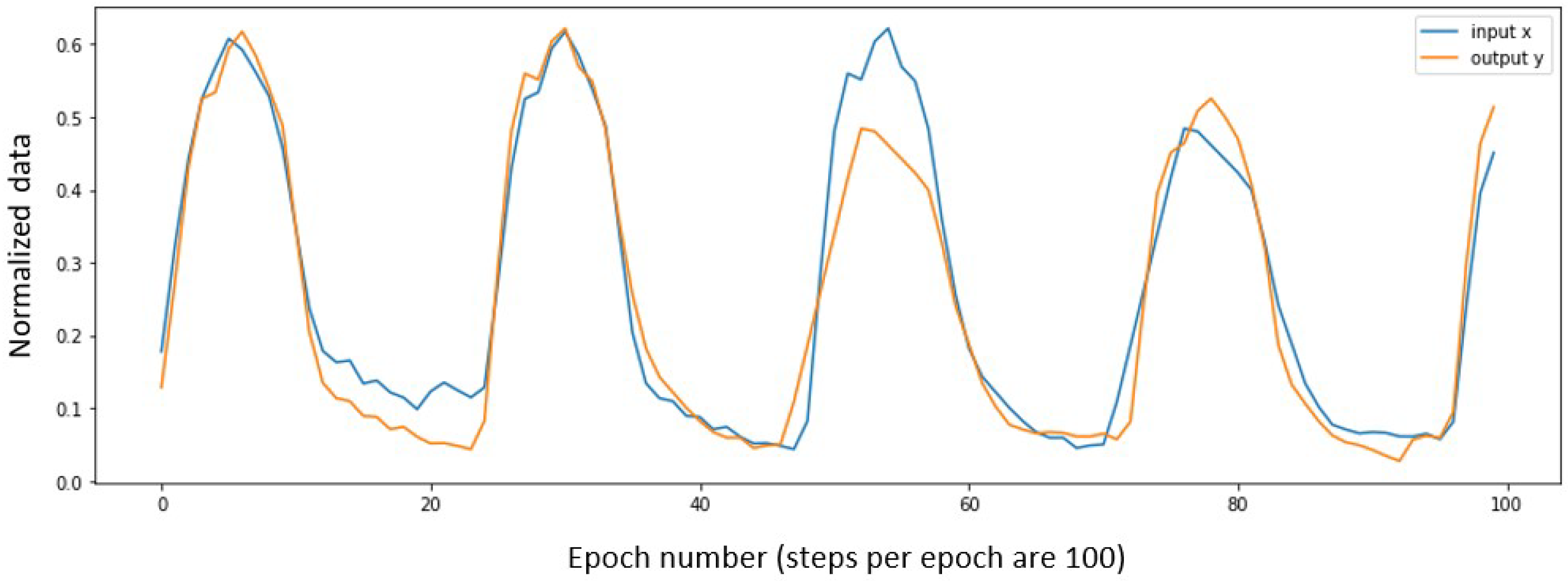
After the collection of the dataset, the first step was normalization. The normalization of data is the removal of repetition and redundancy in data. The data were normalized using a min-max normalization method. The training data is made up of almost eight thousand observations. Instead of training the RNN on the complete sequences of observations, we used a batch of shorter sub-sequences picked at random from the training data. Batch size is the number of training examples utilized in one epoch or iteration. Sequence length represents the number of records in one batch. Lowering the batch size will reduce the size of the data loaded into memory. Lowering the sequence size too much will make the signal history too small to make predictions. For training the model, we chose 20 batch size sets, while the sequence length was set to 24 × 7 × 8, i.e., two-month window used for training.
In
Figure 5, the input (blue curve) and output (orange curve) readings in the graph are shown after setting the step size for model training. The shift steps being set to 24 represents that, as a result of training of model, 24 predicted values will be obtained against each input date.
The neural network trains quickly by running multiple training epochs. However, there is a chance of overfitting the model to the training set, leaving it incapable of oversimplifying the unknown data. Therefore, it is necessary to screen how well the model works on the test data after every epoch and only include the model’s weights if the functioning is enhanced on the test data. The batch generator arbitrarily chooses a batch of small sequences from the training data values and employs it during training. For the validation data value, it is desired to instead route through the complete structure from the test data and measure the prediction correctness on that complete structure. The architecture and number of Training parameters is shown in
Table 2.
To train the neural network, note that a single “epoch” does not correspond to a single processing of the training set because of how the batch-generator randomly selects sub-sequences from the training set. Instead, different researchers have selected steps per epoch in order to process each epoch in a small amount of time. The training of an RNN consists of learning new weight values per epoch. For the modeling of the neural sensor, the defined epochs are 20 and steps per epochs are 100.
3. Results and Discussion
Some conventional testing procedures can be used to evaluate the model’s performance on the test set. This involves examining the model’s anticipated values at various time intervals on the same day. This is a reliable method of demonstrating the neural sensor’s performance. From 1900 to 2200, the prediction is made on an hourly basis.
The results of prediction on the training dataset are shown in
Table 3.
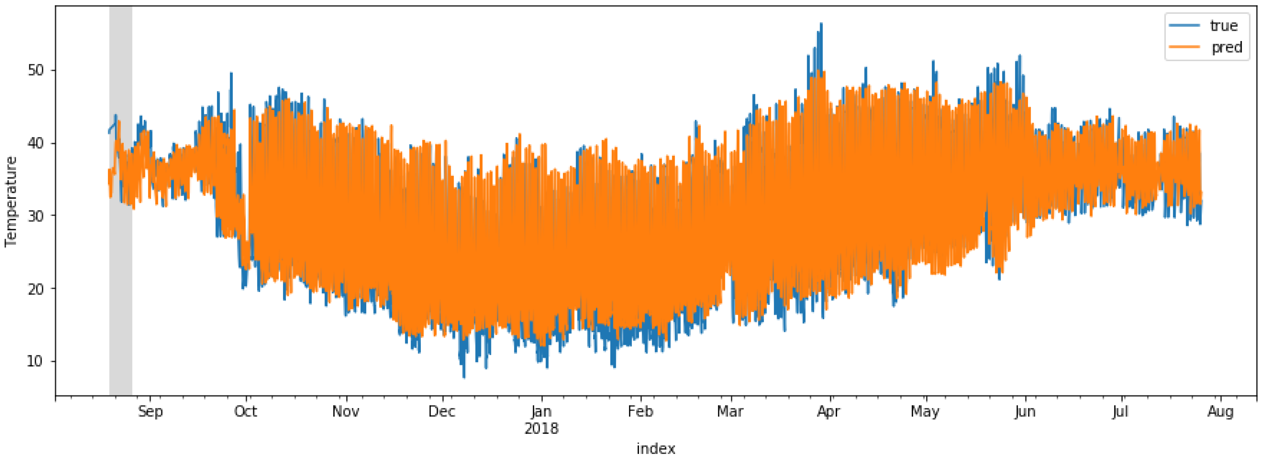
The plot of the predicted output signals is important to understand the workings of the neural sensor in predicting different sensor values. These plots only show the output signals. The time shift between the input and output is fixed. The model foresees the output signals, for example, twenty-four hours into the future (as defined in the shift-steps variable above). Therefore, the x-axis of the plot displays how many time steps of the input-signals have been grasped by the extrapolative model so far.
The prediction is not very accurate for the first 30 to 50 time steps because initially the model has fewer input data at this point. The model generates a single time step of output data for each time step of the input data. The model requires an adequate window of time by processing perhaps 30–50 time steps before it starts generating usable output signals. The initial 50 time steps were ignored, while the mean-squared error in the loss function was calculated, referred to here as the warm-up period. The warm-up period is shown in a grey box in
Figure 6. The blue-colored plot represents the physical sensor values of temperature while the orange-colored plot represents the predicted values of temperature by the neural sensor in
Figure 6. The predicted values are within the acceptable range, except a few spikes between the months of April and January. The created neural sensor, in particular, has shown a high level of overlap with physical sensors utilized from October to April and May to August. This means that the neural sensor learns the patterns of the physical sensor and is able to generate precise predictions.
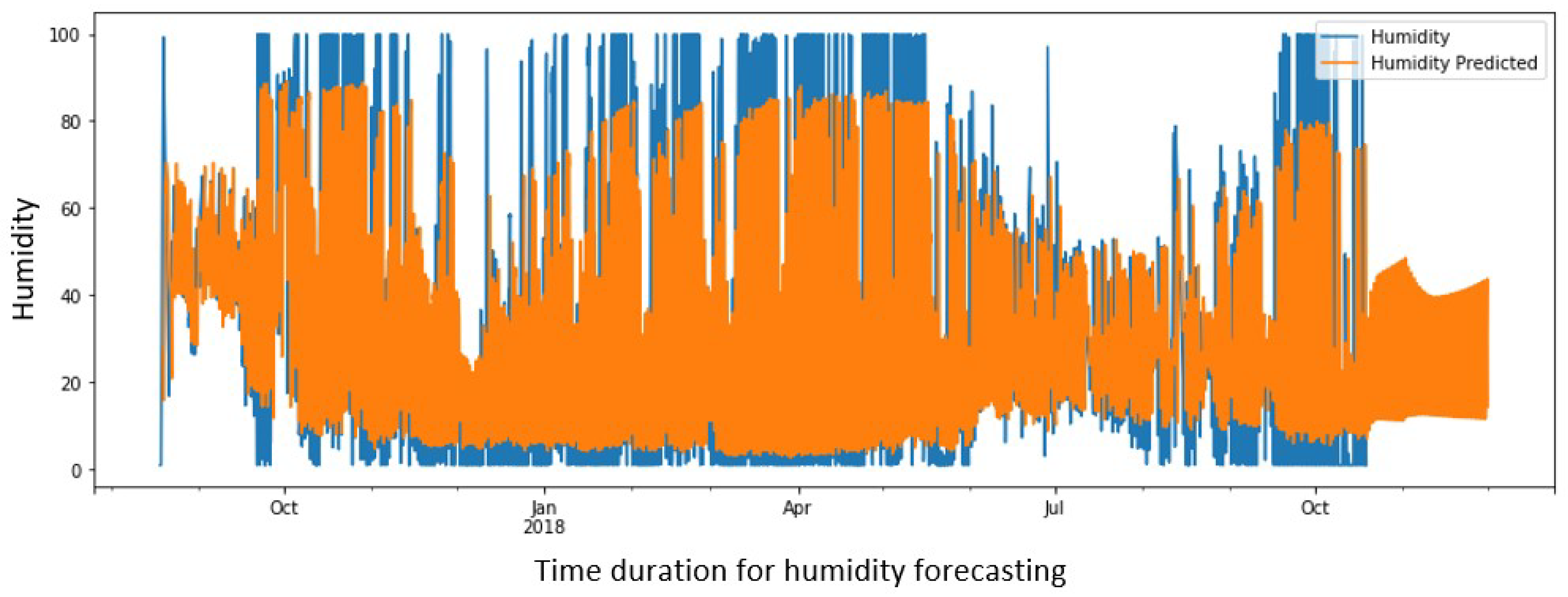
Figure 7 and
Figure 8 show the true and predicted values for humidity and soil moisture, respectively. The performance of the neural sensor well mimics the physical sensor values for humidity compared to soil moisture values throughout the year, despite the fact that the number of spikes in moisture values is slightly greater than that which follows the pattern in the temperature and humidity readings in the test dataset. It was observed that the temperature and humidity predictions successfully overlap with the ground truth dataset, while the moisture value predictions are within an acceptable range for use in agriculture. It should also be noted that all predictions for temperature, humidity and moisture are sensitive to the small changes in values compared to the true values. For instance, the moisture values changed from December to February, as shown in
Figure 8, and are quite small compared to the rest of the ground truth dataset. The observed value differences are minor, as illustrated in
Figure 8, and the suggested neural sensor is capable of measuring the proper moisture values nearly and successfully mimicking the actual values. This is further confirmed in
Figure 6, which shows the temperature readings from September to October, and
Figure 7, which shows humidity readings from September to October and July to August. This demonstrates the neural sensor’s robustness and sensitivity presented in this study.
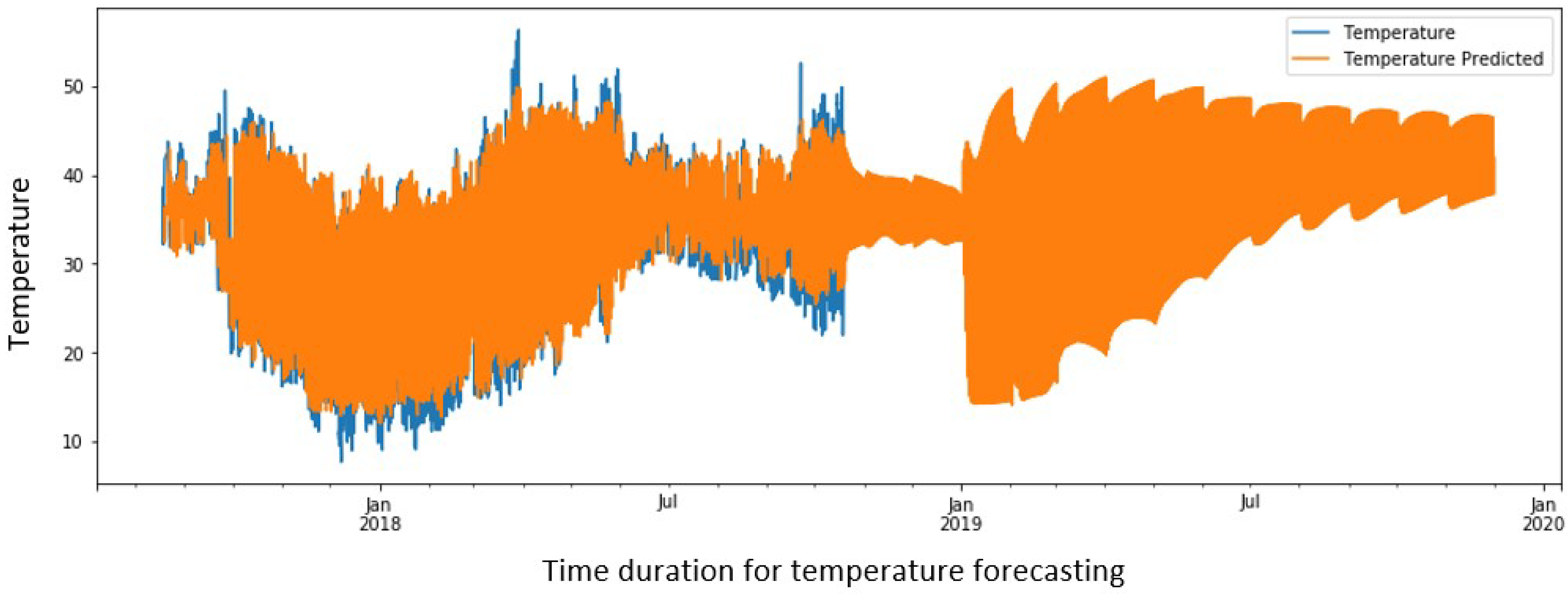
For modeling a neural sensor, a forecasting function is designed which take date as an object to forecast temperature, humidity and soil moisture against that particular date and time, the essential parameter for object (date) is time delta. Time deltas are differences in times. After training of LSTM network, the forecast values of temperature, humidity and soil moisture by neural sensor are shown in
Figure 9,
Figure 10 and
Figure 11, respectively. The blue-colored graph shows the value of the physical sensor embedded in the field and orange curve in the graph is the plot of predicted value of neural sensor that is obtained after the training of the LSTM model.
Figure 9,
Figure 10 and
Figure 11 further confirms the generalization of the proposed neural sensor model and illustrates its potential to be used to complement the physical sensors.
Table 4 presents a statistical analysis where the mean and standard deviation of physical and neural sensors are compared. The mean and standard deviation of physical and neural sensors are very close and show good agreement. Regarding humidity, there is a large standard deviation due to sudden spikes and fluctuation in physical sensor data. The neural sensor does not capture this well. The mean value for physical sensor data is 35.920 and for neural sensor is 30.510. This is due to the sudden rise and fall in physical sensor data values. However, the neural sensor learns after some time and generates reasonable predictions for humidity. For the case of moisture, the behavior of the neural sensor is similar to humidity. We can conclude that the predictions are precise and accurate for temperature and less precise for humidity and moisture.
Table 5 presents a comparison with the related studies. Despite the fact that our work is novel and has not been developed previously in the field of agriculture, we compared the accuracy of our results to other types of neural sensors that mimic the physical sensor behavior for various applications. For instance, for effective sensor array reduction in a gas mixtures analysis system, a neural network sensitivity analysis method was used in [
25], by improving a basic engine parameter, Artificial Neural Network (ANN)-based virtual sensors were employed to manage exhaust emissions and physical sensors can be eliminated during vehicle tuning in [
26], and a convolutional bi-directional LSTM-based approach was proposed in [
27] for a tool wear prediction task as a part of machine health monitoring. Although the applications of neural network models varies, a common goal is to develop an ANN-based sensor to replace physical sensors in a variety of industrial applications. This comparison is conducted based on the accuracy of the models developed in the literature. The accuracy is measured using root mean square values (RMSE). We averaged the RMSE values of temperature, humidity and moisture. The proposed method achieves the best performance within the agriculture sector, compared to other models that are developed for various applications, in terms of accuracy. This research can also be used as a guide for other disciplines looking for alternative solutions, such as medical microrobotics, where physical sensors are difficult to integrate into the system for various measurements such as 3D vibration measurements [
28] and force sensing [
29] for biological cell injection.
The requirement for large datasets to be used as input during the training procedure is a significant limitation of deep learning-based neural sensors that is developed in our study. Furthermore, there are few publicly available datasets for agricultural researchers to work with, so most must create their own datasets, which takes time.
4. Conclusions
The focus of this study is to present a model that addresses the problem of physical sensor nodes malfunctioning by informing the system regarding that particular node. The presented model achieves this by utilizing an alternate mechanism that provides the predictive values of temperature, humidity and soil moisture to avoid instances of complete system failure. The proposed model increased the overall reliability and efficiency of the existing system by providing additional information regarding the working of the physical sensor in the agricultural context. The proposed neural sensor in this paper is successfully able to predict key values related to the SIS system such as temperature, humidity and soil moisture, and is thus able to inform us if the physical sensors embedded in the agricultural field in a real-time environment have malfunctioned.
It also provided a set of predicted values of desired variables for a particular instance on an hourly basis. The current model further provides a mechanism to save the system from complete failure. It helps to improve the mean time to failure of the system and the system performance gradually becomes worse in the case of a malfunctioning physical sensor.
The future possibilities of this research are in the integration of this model with the decision support system of SIS, which decides the supply of water in the field by calculating the amount of water already in the soil with the help of transpiration parameters such as temperature, humidity and soil moisture. This model can be utilized in a number of real-time systems, relying heavily on physical sensor values to avoid any catastrophic event due to the failure/malfunctioning of physical sensor nodes, and to ensure the reliable and safe operation of the system.


