Estimate Cotton Water Consumption from Shallow Groundwater under Different Irrigation Schedules

Abstract

Shallow groundwater is considered an important water resource to meet crop irrigation demands. However, limited information is available on the application of models to investigate the impact of irrigation schedules on shallow groundwater depth and estimate evaporation while considering the interaction between meteorological factors and the surface soil water content (SWC). Based on the Richards equation, we develop a model to simultaneously estimate crop water consumption of shallow groundwater and determine the optimal irrigation schedule in association with a shallow groundwater depth. A new soil evaporation function was established, and the control factors were calculated by using only the days after sowing. In this study, two irrigation scheduling methods were considered. In Method A, irrigation was managed based on the soil water content; in Method B, irrigation was based on the crop water demand. In comparison with Method B, Method A was more rational because it could use more groundwater, and the ratio of soil evaporation to total evapotranspiration was low. In this model, the interaction between meteorological factors and the SWC was considered to better reflect the real condition; therefore, the model provided a better way to estimate the crop water consumption.

1. Introduction

Water scarcity is a great concern for irrigation agriculture worldwide. More than half of the farmland in the world exists in arid and semiarid regions [1]. Irrigation is essential to crop production in arid regions and plays an important role in crop water demands throughout the world. The site-specific application of irrigation water within a field improves water use efficiency and reduces water usage for sustainable crop production, especially in arid and semiarid regions [2].

Rational irrigation scheduling is essential to irrigation management, and many irrigation scheduling studies have been performed in arid regions [3,4,5]. In general, one type of irrigation scheduling is based on evapotranspiration demand, and another is based on the soil water content of the root zone [5]. Shallow groundwater exists in many areas of the world [6], and some farmlands are irrigated with shallow groundwater in arid regions. Shallow groundwater exists in many areas of the world and plays a vital role in sustaining agricultural productivity in many irrigated areas [3,7,8]. Irrational or intensive irrigation leads to a decline in the shallow groundwater table. The variation in a shallow groundwater table strongly influences the water balance [9]. Water cycling in soils with shallow groundwater is complex due to the deep percolation and groundwater evapotranspiration (ET_g) that occur in arid regions [10]. An improved irrigation schedule could reduce the amount of deep percolation [8].

Several studies have used lysimeters to measure crop water consumption from a shallow groundwater table [11,12,13,14,15]. The lysimeters were accurate, but their use is limited because of their high cost [3]. Therefore, some studies have attempted to quantify the groundwater as a part of the SPAC (soil-plant-atmosphere continuum) at the field and regional scales using models such as SWAP [3], EPIC [16], and DSSAT [17]; however, the models mentioned above usually oversimplified the influence of groundwater [18]. Han et al. [18] used the Hydrus-1D model coupled with a simplified crop growth model from SWAT to estimate the effect of groundwater on the water balance in the cotton root zone, but their study did not include a method for irrigation scheduling and was not implemented or systematically used by the majority of growers. Huo et al. [3] simulated the various amounts of irrigation applied to soil with different water tables, but the irrigation schedule was fixed in their study. Therefore, information relative to the irrigation scheduling method is still limited.

Accurate estimations of evapotranspiration (ET) are urgently needed. ET includes soil evaporation (E) and crop transpiration (T); transpiration is considered a physiological process, whereas soil evaporation is a physical process. Soil evaporation is an important component of the total crop water consumption, and the E ratio is higher in the earlier growing season due to wet surface soils and low crop cover (CC) [19]; however, evaporation may be lower in the later growing season when the surface soils are drier, and the CC is higher [20]. Unkovich et al. [20] reviewed the published field measurements from Australia and found an average of 38% crop water consumption due to soil evaporation. Kool et al. [21] noted that the E/ET ratio exceeded 30% in 32 of the studies and noted that E usually constituted a large fraction of ET and should be independently considered. Numerous measurement methods and analytical models have been developed to estimate T and E separately, but large variability exists in ET partitioning, suggesting that obtaining accurate ET partitioning is relatively challenging [21]. In general, T is controlled by atmospheric evaporative demand, leaf area index (LAI) or crop cover (CC), surface soil water content (SWC), and reference crop evapotranspiration (ET₀) [22,23,24,25]. These factors influence T and E, as well as ET partitioning. Therefore, most previous studies focused on the influence of crops on ET partitioning using regression functions between CC and T/ET or E/ET [26,27,28,29,30]. Zhao et al. [25] established a function between ET partitioning and control factors (CC and SWC), but the metrological factors were neglected, and the CC and SWC had to be acquired by field experiment observations. The establishment of simple functions that are correlated with the main control factors without field experiment observations was necessary. It will provide a better way to interpret evapotranspiration partitioning and to model water consumption in cotton fields.

Existing models include Hydrus-1D; however, E or SWC must be acquired by field experimental observations. For SWC, E is just an input parameter, leading to the interaction between SWC and E being neglected. However, this interaction effect is present. For example, a high soil water content could cause high soil evaporation, but meteorological factors also influence the SWC [20,21]. If the SWC or E are included as only input parameters, then the interaction effect will be neglected, and the real condition will not be reflected. Although the HYDRUS model can simulate irrigation and water consumption at a given groundwater table, the model can only set a fixed or initial groundwater table. In practice, changes in groundwater table are not entirely dependent on evaporation consumption from cropland (but lysimeter with impermeable bottom) but involve lateral recharge and groundwater consumption from surrounding areas. Our model takes into account an actual groundwater change (groundwater variation with time as an input parameter), which better reflects a real situation. Therefore, in this study, we developed a model to estimate crop water consumption and considered an actual groundwater table fluctuation and the interaction between SWC and E.

The objective of our research was to (1) develop a model based on the Richards equation to simultaneously estimate crop water consumption with shallower groundwater, (2) develop a new function for estimating soil evaporation considering the interaction between SWC and E, (3) validate this model using cotton field experiment observations, and (4) apply the new tool to estimate a suitable irrigation schedule.

2. Materials and Methods

2.1. Mathematic Model

2.1.1. Water Flow Equations

The Richards model was used to simulate the soil water movement as follows [31]:

$$\{\begin{array}{l}\frac{\mathit{\partial }\theta }{\mathit{\partial }t}=\frac{\mathit{\partial }}{\mathit{\partial }z}\left[K\left(\frac{\mathit{\partial }h}{\mathit{\partial }z}+1\right)\right]-S,0\le z\le L_r\\ \frac{\mathit{\partial }\theta }{\mathit{\partial }t}=\frac{\mathit{\partial }}{\mathit{\partial }z}\left[K\left(\frac{\mathit{\partial }h}{\mathit{\partial }z}+1\right)\right],L_r\le z\le L\end{array}$$

(1)

where $S$ is the root water uptake (cm⁻¹), $h$ is the pressure water head (cm), $\theta$ is the soil water content (cm³ cm⁻³), $L_r$ is the crop root zone depth (cm), $L$ is the soil depth (cm), and $K$ is the unsaturated hydraulic conductivity (cm day⁻¹). The van Genuchten–Mualem model was used to estimate the soil hydraulic properties [32].

2.1.2. Root Water Uptake

The root water uptake is described as follows [33]:

$$S=\alpha \left(h\right)\times b\left(z\right)\times T_p\left(t\right)$$

(2)

where $\alpha \left(h\right)$ is the soil water stress response function [34]. The parameters in the Feddes et al. [34] model for cotton are $h_1$ = −10 cm, $h_2$ = −25 cm, $h_{3max}$ = −200 cm, $h_{3min}$ = −600 cm, and $h_4$ = −14,000 cm [35,36], $b\left(z\right)$ is the root water uptake distribution function [37] and $T_p\left(t\right)$ is the cotton actual transpiration during one day (cm), which was calculated as follows [4]:

$$T_p\left(t\right)=E{T}_p\left(t\right)\times \left(1-exp\left(-\gamma \left(1+\delta \left|sin\frac{\pi \left(t_d-S_N\right)}{12}\right|\right)LAI\right)\right)$$

(3)

where $E{T}_p\left(t\right)$ is the potential evapotranspiration of cotton (cm day⁻¹), which was calculated using the FAO 56 Penman–Monteith equation [38], $LAI$ is the leaf area index and is a function of the time after sowing, $\delta$ and $\gamma$ are the empirical coefficients, $t_d$ is time (h), and $S_N$ is time at noon (h).

2.2. Field Experiment and Model Parameterization

2.2.1. Study Area

This experiment was conducted at the Aksu National Field Research Station of Agroecosystems (40°37′ N, 80°51′ E) in the northwestern Tarim Basin, Xinjiang Province, China. Cotton was the main crop, which is largely dependent on irrigation. The precipitation was variable with a mean value of 45.7 mm, the annual pan evaporation was approximately 2500 mm, and the mean temperature was approximately 8 °C. The groundwater table is shallow and approximately 2 m. The soil physical properties at the experimental site are shown in

Table 1. Soil bulk density and particle size distribution from 0 to 80 cm in experiment sites.

Depth (cm)	Bulk Density (g/cm3)	Soil Particle Size Distribution (%)
		<0.002 mm	0.002–0.05 mm	0.05–2.0 mm
0–10	1.33	8.03	78.8	13.17
10–20	1.37	8.36	80.32	11.32
20–40	1.5	11.56	82.32	6.12
40–60	1.44	13.7	83.21	3.09
60–80	1.41	9.42	75.96	14.62

.

2.2.2. Field Experimental Design

The experiment was conducted in 2010 and 2011, and the plot area was 150 m × 90 m. The cotton was sown in April and harvested in November. The phenological phases of cotton growth are shown in

Table 2. Phenological phases of cotton growth in 2010 and 2011.

Phenological Phases	2010	2011
Seeding	30 April 2010	5 May 2011
Emergence stage	2 May 2010	5 May 2011
Squaring stage	10 June 2010	12 June 2011
Flowering stage	3 July 2010	28 June 2011
Boll opening stage	25 August 2010	19 September 2011
Harvest	1 November 2010	2 November 2011

, and the irrigation schedule is shown in

Table 3. The rainfall date and irrigation schedules in 2010 and 2011 in cotton field.

Irrigation Date	Irrigation Amount (mm)	Rainfall Date	Rainfall Amount (mm)	Rainfall Date	Rainfall Amount (mm)
25 June 2010	180	5 June 2010	1.6	25 October 2010	15.7
12 June 2010	100	12 June 2010	0.2	31 October 2010	0.6
2 August 2010	150	16 June 2010	0.4	5 May 2011	4.8
29 August 2010	130	20 June 2010	0.3	10 May 2011	3.2
30 June 2011	199	25 June 2010	0.3	15 May 2011	4.4
15 July 2011	240	31 June 2010	3.0	20 May 2011	0.6
9 August 2011	148	20 August 2011	1.8	5 June 2011	2.6
25 August 2011	157	25 August 2010	0.5	20 June 2011	8.2
		20 September 2010	2.3	15 August 2011	3.1
		26 September 2010	11.2	19 August 2011	1.5
		29 September 2010	7.8	5 September 2011	2.3

. Additional spring and winter irrigation was applied before seeding and after harvest, providing approximately 200 mm of water to leach the salt.

2.2.3. Measurements

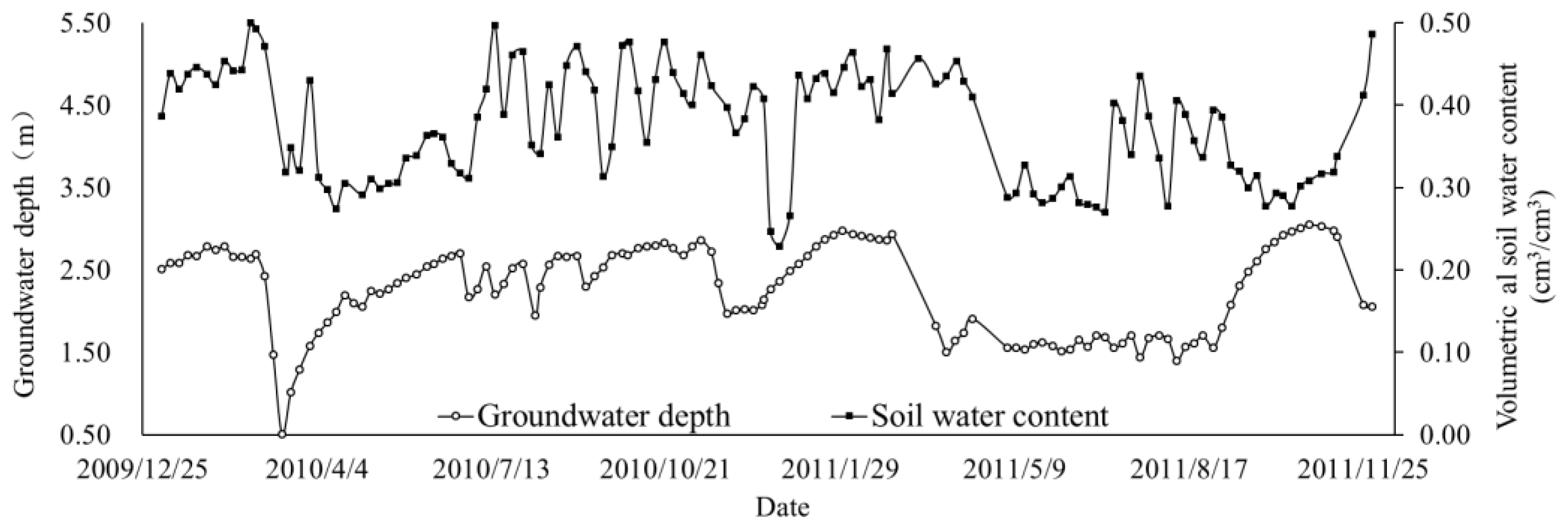
The soil water content and groundwater table were observed every 5 days (Figure 1). The soil water content was measured using a neutron probe (CNC503DR, Beijing Hean Nuclear Instrument Company, Shenzhen, China) with three replications at depths of 10, 20, 30, 40, 50, 70, 90, 110, 130, and 150 cm. This neutron probe consists of two main components: a probe and a rate meter. The density of slow neutrons formed around the probe is nearly proportional to the concentration of hydrogen in the medium of the probe. Equation (4) was used to calculate soil water content:

$$\theta =0.615\frac{R}{R_w}+0.0289, r=0.952$$

(4)

where $R$ was the slow neutron count in soil, and $R_w$ was standard neutron count.

The groundwater table was measured using a water level scale every 5 days. An automatic meteorological station was installed in the field to measure wind speed (Model 010c, Met One, Grants Pass, OR, USA), solar radiation (Model LI200X, Campbell Scientific, Logan, UT, USA), precipitation (Model 52202, RM Young, Traverse City, MI, USA), air temperature, and relative humidity (Model Hmp45c, Campbell Scientific, Logan, UT, USA), and a datalogger (Model CR1000, Campbell Scientific, Logan, UT, USA) was used to monitor the sensors. Leaf samples were collected with five replications for each phenological phase, and the LAI was calculated by the leaf width (W) and length (L) [39], the mean LAI was 0.16 (std, 0.01), 0.92 (std, 0.03), 2.91 (std, 0.16), 3.23 (std, 0.33), and 1.76 (std, 0.15) from emergence to harvest stage, respectively.

2.2.4. Numerical Modeling

The initial conditions were set based on the soil moisture. The bottom boundary was assigned at the pressure head boundary condition using the observed groundwater table depths, and the upper boundary was set according to the atmospheric boundary condition as follows [33]:

$$\frac{\mathit{\partial }\theta }{\mathit{\partial }t}=-\frac{\mathit{\partial }q}{\mathit{\partial }x}$$

(5)

where $q$ is the soil surface water flux. If the soil surface is flooded, $q=I\left(t\right)$, $I\left(t\right)$ is infiltration rate, and if the soil surface water has begun to evaporate, the $q=E\left(\theta \right)$, where $E\left(\theta \right)$ is the evaporation intensity.

We defined the five soil layers (0–10, 10–20, 20–40, 40–60, and 60–80 cm) in the soil profile (Table 1) based on previous studies [18]. The soil hydraulic parameters of the van Genuchten–Mualem model are shown in

Table 4. Soil hydraulic parameters of the van Genuchten–Mualem model at the experimental site.

Depth (cm)	θr (cm3/cm3)	θs (cm3/cm3)	α (cm−1)	n	Ks (cm·day−1)
0–10	0.0563	0.43	0.0050	1.70	25
10–20	0.057	0.42	0.0053	1.68	15
20–40	0.0062	0.41	0.0062	1.63	9
40–60	0.0671	0.44	0.0059	1.64	6
60–270	0.055	0.41	0.0053	1.68	5

, and the parameters remained constant for both model calibration and validation. The pore connectivity parameter was constant (0.5). The parameter estimation tool (PEST) [40] was used to optimize the parameters ${\theta }_r$, $\alpha$, $n$, $\gamma$ and $\delta$. The time from 30 April to 31 October in 2010 and the time from 2 May to 2 November in 2011 were used to calibrate t and validate the model, respectively. The optimized parameters of the van Genuchten–Mualem analytical functions [32] are given in Table 4, with γ = 0.7937 and $\delta$ = 0.10364.

Soil evaporation is also controlled by meteorological factors and the CC. The CC was adequately described by the logistic growth curve with the days after sowing (t), and $E{T}_0$ reflected the meteorological factor; thus, we were able to establish the function by combining the $E{T}_0$ and CC to calculate the soil evaporation as follows:

$$E\left({\theta }_{top}\right)={\left(a_1{\theta }_{top}+a_2\right)}^{a_3}\times {\left(E{T}_0\right)}^{a_4}\times \left(1+exp\left(-a_{5}t\right)\right)$$

(6)

The constants $a_1$, $a_2$, $a_3$, $a_4,$ and $a_5$ were obtained by fitting the parameters with observed data, and they were 1.3181, 0.3400, 8.4880, 0.1282, and 1.5734, respectively. The R² was 0.77, and the RMSE was 0.049. ${\theta }_{top}$ represents the mean soil water content (0–5 cm). This equation does not include a measured parameter “CC”; the CC was reflected by the last term (power function).

The relationship between the $LAI$ and the days after sowing is expressed in Equation (6), with R² = 0.99 and RMSE = 1.15:

$$LAI\left(t\right)=-4.64\times {10}^{-3}+2.89\times {10}^{-2}t-1.48\times {10}^{-3}{t}^2+3.27\times {10}^{-5}{t}^3-1.70\times {10}^{-7}{t}^4$$

(7)

2.3. Model Solutions

The soil to a depth of 2.7 m was simulated, and the grid size was 0.01 m. Equation (1) was solved using the finite-element method, and the solutions were the same as those of the Hydrus-1D model [33]. A software package (MATLAB 7.0 for Windows) was used to edit the code.

2.3.1. Model Evaluation

The correlation coefficient (R²) and the root mean square error (RMSE) were used to evaluate the agreement between the simulated results and the observed results:

$$\mathrm{RMSE}={\left[\frac{1}{n}{{\displaystyle \sum }}_{i=1}^n{\left(C_{si}-C_{ob}\right)}^2\right]}^{1/2}$$

(8)

$${\mathrm{R}}^2={\left[\frac{{{\displaystyle \sum }}_{i=1}^n\left(C_{si}-\overline{C_{si}}\right)\left(C_{ob}-\overline{C_{ob}}\right)}{{{\displaystyle \sum }}_{i=1}^n\left(C_{si}-\overline{C_{si}}\right){{\displaystyle \sum }}_{i=1}^n\left(C_{ob}-\overline{C_{ob}}\right)}\right]}^2$$

(9)

where C_si is the model prediction at time interval i, C_ob is the field observation, n is the total number of observed values, $\overline{C_{si}}$ is the mean of the simulated values, and $\overline{C_{ob}}$ is the mean of the observed values.

2.3.2. Sensitivity Experiments

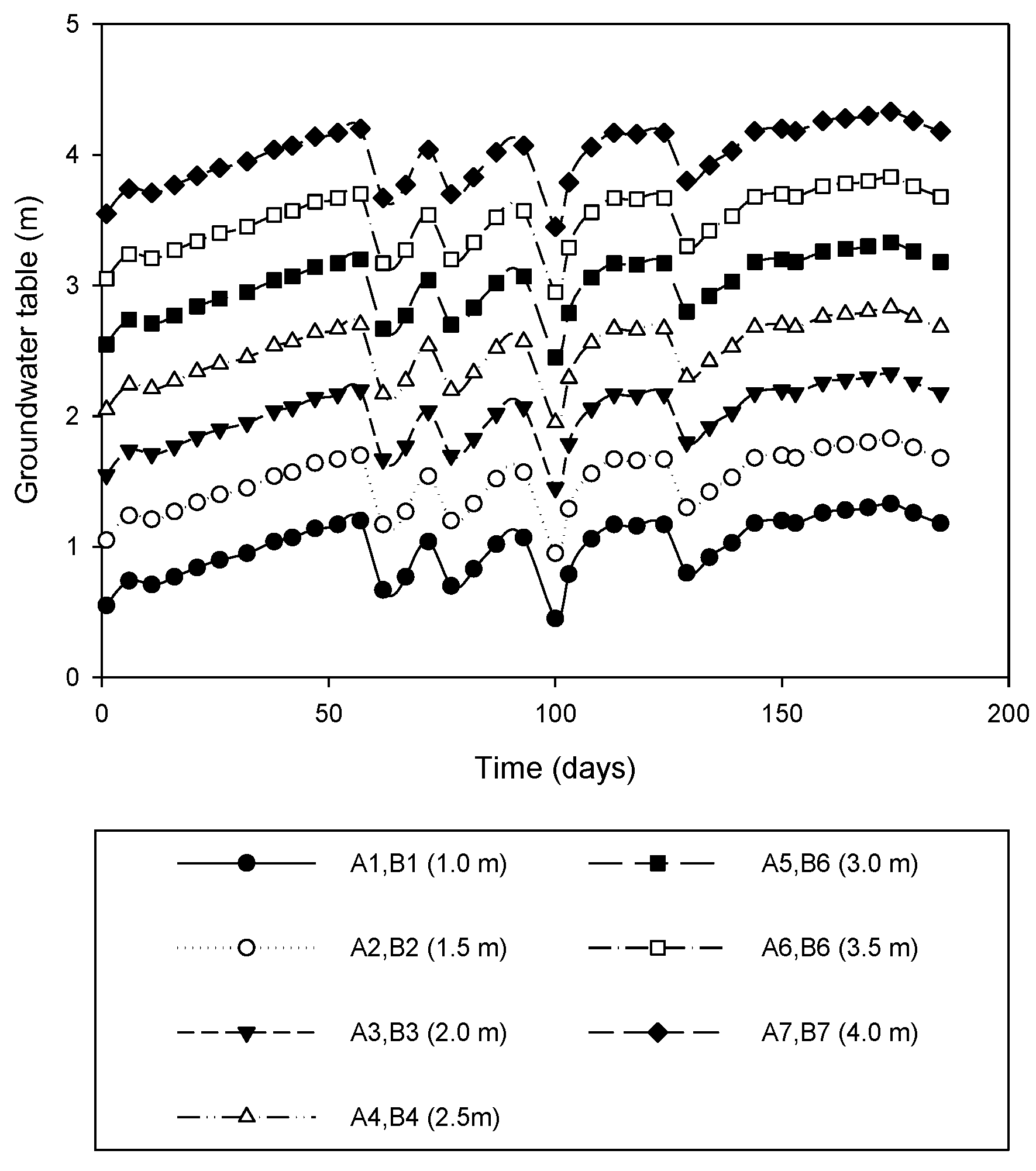
The numeric simulation experiments were mainly conducted to determine the influence of the irrigation schedule and groundwater depth on the soil root zone water balance. The effects of the irrigation schedule and groundwater table depth on the water capacity, capillary rise, actual evaporation, and actual transpiration were estimated. The root zone was from the surface soil (0 cm) to a depth of 60 cm. Fourteen different modeling scenarios were considered (

Table 5. The 14 different modeling scenarios included the seven groundwater depths and two irrigation schedules for the numerically simulated experiments.

Irrigation Schedule		Groundwater Depth (m)
Method A	Method B
Irrigation Managed Based on the Soil Water Content	Irrigation Was Based on the Crop Water Demand
A1	B1	1.0
A2	B2	1.5
A3	B3	2.0
A4	B4	2.5
A5	B5	3.0
A6	B6	3.5
A7	B7	4.0

). The groundwater table fluctuation had a range from 1.4 to 3.1 m during the growing season in 2010 and 2011 (Figure 1). The modeling scenarios cover this range to reflect the real situation; thus, we conduct seven groundwater tables from 1.0 to 4.0 m.

We assumed that the groundwater table was a natural fluctuation, which was not entirely influenced by water consumption from cropland. It can be seen in Figure 1, which was the observed variation of the groundwater table with time. The variation trend does not show a strong relation with irrigation or water consumption. For each scenario, the groundwater table time series were generated by adding a constant value (ranging from −1.5 to 1.5 m) to the groundwater table depth measured in 2010. It was an input parameter to run the model (Figure 2). The mean groundwater table was 2.5 m (measured value during growing season) in 2010, the seven groundwater table (mean value) were conducted as follow: 1.0 m (2.5 m + (−1.5 m)), 1.5 m (2.5 m + (−1.0 m)), 2.0 m (2.5 m + (−0.5 m)), 2.5 m (2.5 m + 0 m), 3.0 m (2.5 m + 0.5 m), 3.5 m (2.5 m + 1.0 m), and 4.0 m (2.5 m + 1.5 m) (Table 5), respectively, all the change trend of groundwater tale (14 treatments) were consistent with measured data in 2010 during growing season (Figure 2). Two common irrigation scheduling methods were selected. In Method A, the irrigation was managed based on the soil water content, and the lower limits of the controlled soil water contents at field capacity (θ_f) were 0.55θ_f, 0.6θ_f, and 0.7θ_f for the planned soil moisture layers of 0.2 m, 0.4 m, 0.6 m and 0.8 m in the emergence stage and squaring stage, respectively. The higher limit of the soil water contents at field capacity was 0.95. With Method B, the irrigation amount and timing were designed based on the crop water demand (local farmer custom), depending on the potential ET in the next N (or 20) days.

3. Results and Discussion

3.1. Model Calibration and Validation

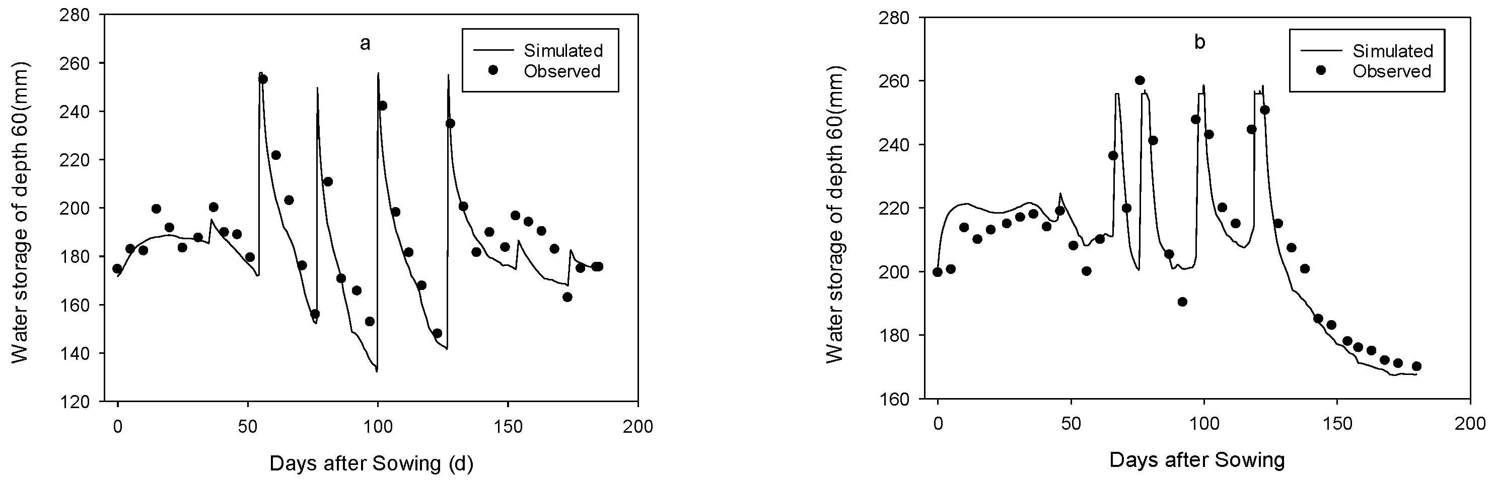
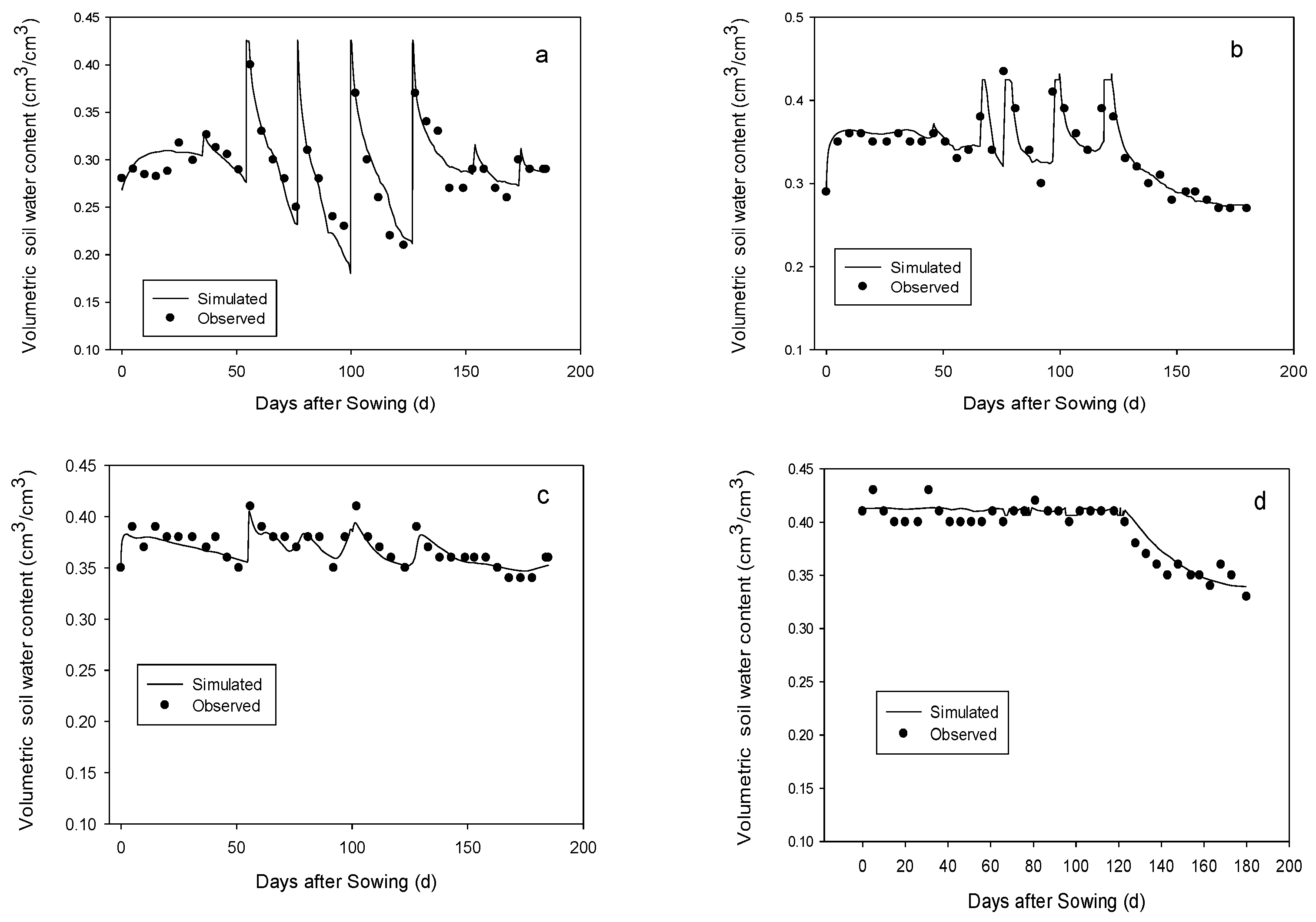
The relationship between the measured and simulated soil water storage in the root zone (0–60 cm) is shown in Figure 3. Suitable agreement between the measured and simulated values (soil water storage) was found. The model slightly overpredicted the water content during the calibration process; on the contrary, the validation process showed slight underprediction. More statistical tests were conducted to evaluate the performance of the model. The simulated and measured soil water contents from the soil depths of 20 and 150 cm are shown in Figure 4, which indicates that the predicted values are in agreement with the observed values. The R² and RMSE values for the soil water contents and soil water storage (0–60 cm) are shown in

Table 6. Statistical tests for the modeling results in 2011 and 2012.

Period	Year	Item	Soil Water Content (−)	Soil Water Storage (mm)
Calibration process	2010	R2	0.92	0.93
		RMSE	0.04	20.83
Validation process	2011	R2	0.94	0.93
		RMSE	0.04	24.06

. The R² values ranged from 0.92 to 0.94, the RMSE values of the soil water storage at 60 cm, and the soil water content were 20–24 mm and 0.04, respectively. These statistical tests indicated that the model had suitable performance.

3.2. Scenario Simulation

3.2.1. Soil Water Storage Variation in the Root Zone

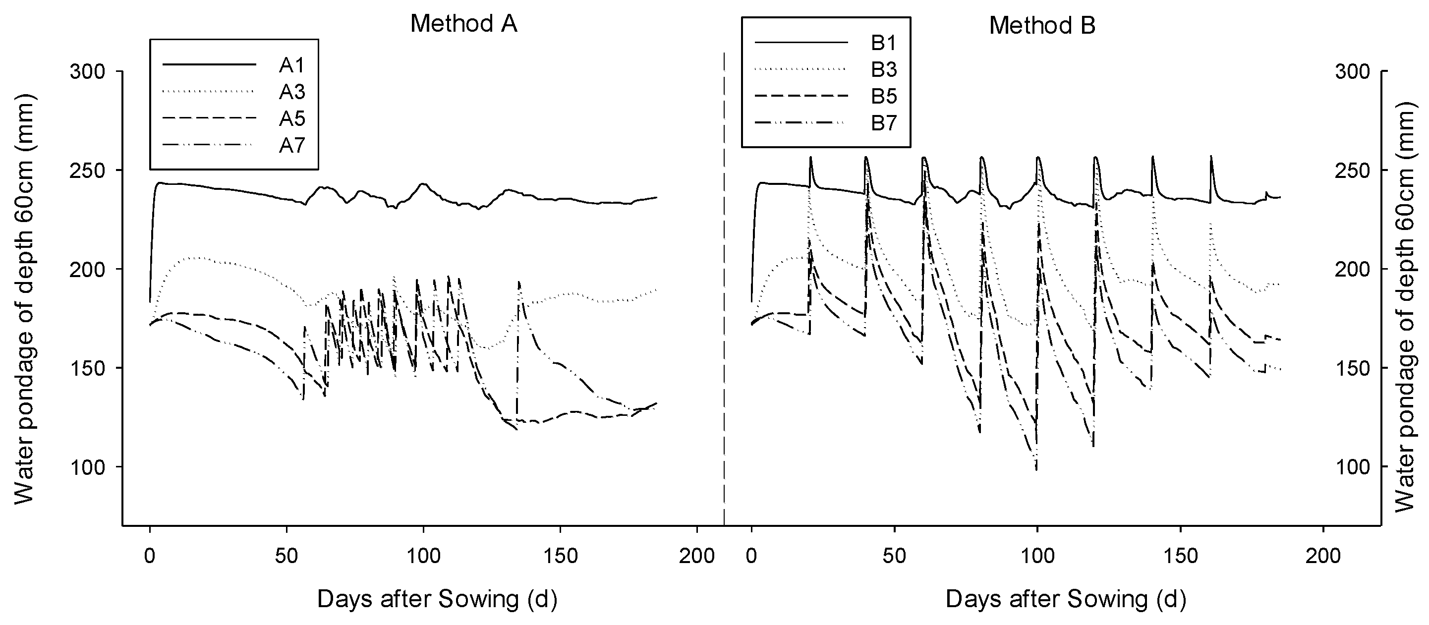
The soil water storage in the root zone (0–60 cm) showed variations under the different treatments (Figure 5). The soil water storage showed sharp increases after irrigation and then decreased gradually due to percolation and evaporation. When the groundwater table was shallow, the soil water storage showed small variations with high values because the groundwater could supply water into the soil root zone. In contrast, when the groundwater table was deep, the water supply from the groundwater was weaker and could not satisfy the water consumption by the cotton, which caused low soil water content in the root zone, deepened the groundwater table, and caused greater fluctuations in the soil water content.

In general, shallow groundwater is considered a water resource for crop irrigation. In our research, the irrigation times increased from treatment A1 (1.0 m) to A7 (4.0 m) with the increase in groundwater depth. The groundwater table was maintained at depths of 1.0 (treatment A1) and 1.5 m (treatment A2), and the groundwater was able to supply enough water to the root zone for evaporation (Figure 6 and

Table 7. The simulated irrigation schedule for 14 treatments.

Treatments	Irrigation Schedule	Irrigation Time (d)/Irrigation Amount (mm)											Total
A1	Irrigation time	0
	Irrigation amount	0											0
A2	Irrigation time	0
	Irrigation amount	0											0
A3	Irrigation time	89
	Irrigation amount	42											42
A4	Irrigation time/(d)	65	74	82	89	105
	Irrigation amount	35.00	36.75	40.25	42.00	47.25							201.25
A5	Irrigation time	64	70	77	83	89	97	109
	Irrigation amount	46.55	35.00	38.50	40.25	42.00	45.50	49.00					296.8
A6	Irrigation time	60	66	71	77	83	88	96	103	112	141
	Irrigation amount	41.65	35.00	36.75	38.50	40.25	42.00	43.75	47.25	49.00	72.80		446.95
A7	Irrigation time	56	65	69	74	80	85	90	97	103	112	134
	Irrigation amount	39.20	35.00	35.00	36.75	38.50	40.25	42.00	45.50	47.25	49.00	75.60	484.05
B1–B7	Irrigation time/(d)	20	40	60	80	100	120	140	160	180
	Irrigation amount	38.31	73.79	103.75	97.21	90.89	106.88	45.85	34.44	3.72			594.84

). The groundwater table does not show a significant decrease (Figure 2); therefore, irrigation was not necessary with a shallower groundwater table (1.0 and 1.5 m). Kahlown et al. [14] investigated the water tables that were maintained at shallower depths (e.g., 0.5 m for wheat) and noted that the groundwater could meet the crop water requirements, but differences were observed for different crops [14] and soil textures [3]. For treatment A7, the first irrigation occurred on the 56th day. This is because the soil evaporation was small due to low surface soil water content, which led to low soil evaporation. Usually, the surface soil water content showed a strong influence on soil evaporation, which has been reported in many studies [41,42,43]. The dry surface soils lead to vapor transport through the surface [44], which will be greatly inhibited the soil evaporation, thus retained the water in below the surface. The cotton was seeding around at depth of 5 cm, thus it could obtain the water by root at the emergence stage.

For Method B (Treatments B1 to B7), the irrigation amounts and times were similar among the treatments (Table 7). Compared with Method A, the soil water storage (0–60 cm) in Method B showed more significant fluctuations (Figure 5). Method B had fixed irrigation times and amounts, and the soil water potential was higher in the root zone than in the lower layer after irrigation and resulted in downward soil water movement. In contrast, irrigation began when the soil water content reached the prescribed lower limit; therefore, the soil water potential was lower in the root zone than in the low layer, causing the groundwater to move upward into the root zone (Figure 6).

3.2.2. Evapotranspiration Dynamics

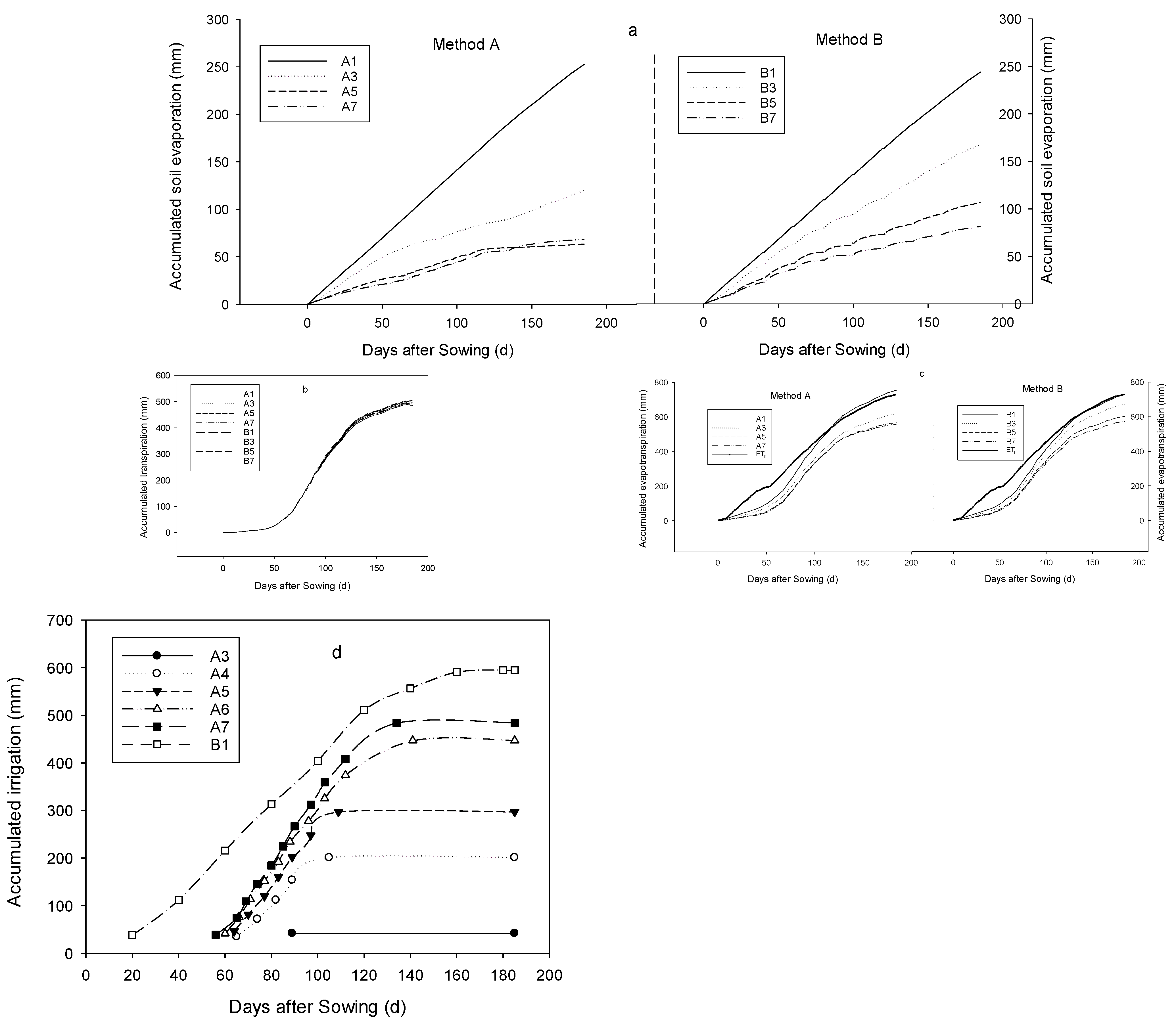
Figure 6 shows the accumulated soil evaporation, transpiration, evapotranspiration, ET_0, and irrigation amounts under the different treatments. The amount of soil evaporation was larger when the groundwater table was shallower, with the soil evaporation reaching 252.6 and 244.1 mm at a depth of 1.0 m and reaching only 68.5 mm and 81.5 mm at a depth of 4.0 m for Method A and Method B, respectively (Figure 7a). However, the cotton transpiration was not significantly different for the different groundwater tables and irrigation methods, showing a range from 485.0 to 505.7 mm for all treatments, and the amounts of T and E were similar in the two irrigation methods (Figure 7a,b). Except for the seeding and emergence stages, cotton transpiration was less than soil evaporation because of the small CC. However, after the emergence stage, the increased, causing larger cotton transpiration and smaller soil evaporation. As the irrigation amount and time increased, the soil evaporation and transpiration showed increasing trends (Figure 7d), but the variation in transpiration was small. This trend occurred because the soil evaporation was higher after irrigation and resulted in increased soil evaporation. The soil evaporation variation trend was similar to the variation pattern.

As mentioned above, cotton transpiration was strongly correlated with meteorological factors and was also correlated with the irrigation amount and soil water content. Cotton transpiration was described by the logistic curve (Figure 7b), with cotton transpiration greater than soil evaporation, but the soil evaporation increased significantly or was higher than transpiration after irrigation, indicating that the irrigation had a great influence on the soil evaporation. The ET₀ was calculated using the meteorological factor by the FAO 56 Penman–Monteith equation [38]. The ET₀ directly reflects the evaporation demand by ambient conditions. The high ET₀ in the early stage is due to the increase in evaporation demand (temperature and radiation), while the actual evaporation (evapotranspiration) is controlled by the soil surface water content, and the crop transpiration is small at this stage. Therefore, the high ET₀ in the early stage but the evapotranspiration smaller than ET₀ (Figure 7c). With the cotton growing, the cotton transpiration increased significantly (Figure 7b), the evapotranspiration is gradually close to ET₀ and has the same trend, indicating that the evapotranspiration was dominated by cotton transpiration after the flowering stage.

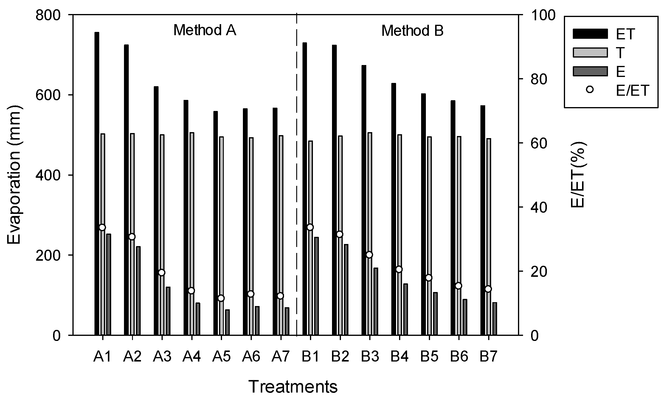
Ding et al. [45] found that higher soil evaporation occurred in early growing seasons due to the small canopy in the maize field, particularly after rainfall or irrigation events. The wet soil surface may have caused increased soil evaporation, and the soil evaporation gradually decreased as the soil dried [25]. Our research results were similar to the results of these studies. The soil evaporation was approximately 11% to 34% of the total evapotranspiration, and the soil evaporation was noticeably reduced with a shallower groundwater table and less irrigation. The soil evaporation was influenced by the groundwater table and showed some differences with the irrigation times and different groundwater table depths. The surface soil was relatively wet when the groundwater table was shallow (e.g., 1.0 m), and the soil evaporation was approximately 33% of the total evapotranspiration. For the deeper groundwater table depth in Method B, the ratio (E/ET) showed a decreasing trend from 33% to 14%, whereas for Method A, the soil evaporation was only 11% of the total ET, with treatment 5 showing the smallest ratio of all treatments (Figure 8).

As noted above, previous studies have presented some regression functions between CC or LAI and T/ET or E/ET to obtain the ET partition [26,27,28,29,30]; however, some functions neglected metrological factors. As mentioned above, the SWC or E was the input parameter, and some parameters, including CC, must be acquired by field observations, while the interaction effect was neglected. Our functions (Equation (5)) were established in correlation with the SWC, CC, and meteorological factors, and the parameter was calculated by days after sowing (Equation (6)), considering the interaction effect. Therefore, we provided a better way to reflect evapotranspiration partitioning and to model water consumption in a cotton field.

3.2.3. Water Balance in the Root Zone

Table 8. The water balance component under 14 treatments.

Simulated Treatments	ET/mm	T/mm	E/mm	ETg/mm	Soil Water Consumption/mm	Irrigation Amount/mm	Irrigation Times	Error/%
A1	755.23	502.66	252.57	826.36	−52.90	0.00	0	−2.41
A2	724.00	503.09	220.91	780.66	−41.65	0.00	0	−2.07
A3	620.01	500.01	120.00	610.80	−17.98	42.00	1	−2.39
A4	585.86	505.65	80.20	383.96	8.93	201.25	5	−1.41
A5	558.09	494.75	63.34	238.12	39.53	296.80	7	−2.93
A6	564.76	493.05	71.72	100.54	31.21	446.95	10	−2.47
A7	566.80	498.33	68.48	55.71	42.10	484.05	11	−2.66
B1	729.11	484.99	244.12	199.63	−52.94	594.84	9	−1.70
B2	723.59	497.14	226.46	179.97	−42.43	595.85	9	−1.35
B3	672.99	505.43	167.56	118.33	−20.86	593.22	9	−2.63
B4	628.12	500.22	127.90	48.33	−4.58	595.85	9	−1.83
B5	602.00	495.26	106.74	−5.99	7.44	593.98	9	1.09
B6	585.00	495.89	89.11	−26.54	16.35	595.85	9	−0.11
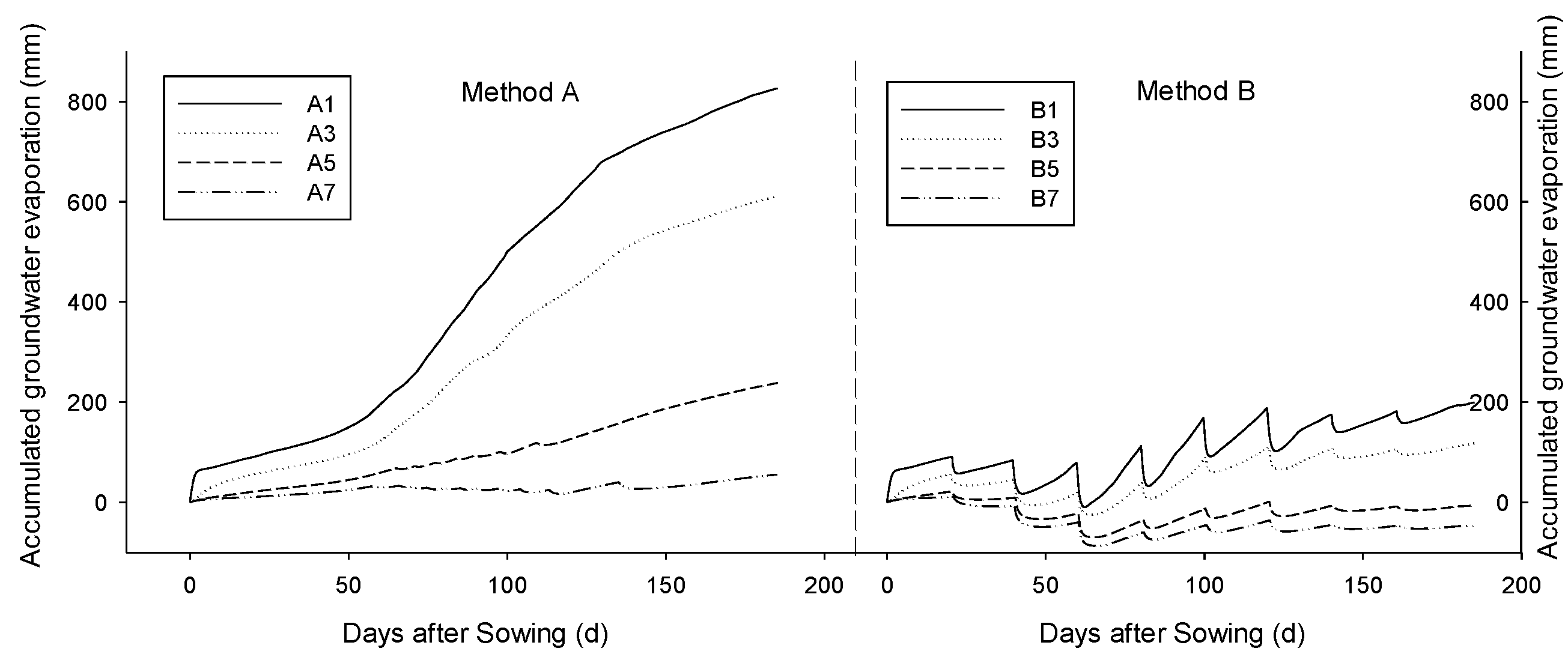
B7	572.61	491.09	81.52	−46.12	23.17	594.84	9	0.13

shows the water balance in the root zone, including evapotranspiration, soil evaporation, cotton transpiration, and soil water and groundwater evaporation. The relative error was less than 3%, which indicates that the model performs well when quantifying the water balance in the cotton field. The cotton water consumption showed great differences under the different treatments. For example, the source of cotton water consumption was mainly derived from the groundwater when the groundwater table was shallower in Method A, but the source gradually transformed to irrigation when the groundwater table was deeper. The cotton water consumption was 826 mm when the groundwater table remained at a depth of 1 m, almost meeting the cotton water demands. When the groundwater table was deeper, the groundwater evaporation decreased gradually. The groundwater evaporation sharply decreased to below 2.5 m. The groundwater evaporation was 383 mm at 2.5 m, which only partially met the cotton water consumption demand.

The simulated evapotranspiration ranged from 558 to 755 mm, but the cotton transpiration ranged from 485 to 505 mm. The irrigation of cotton was not necessary when the groundwater table was less than 1.5 m deep because the water source for cotton consumption mainly came from the groundwater. The irrigation amount was greater than 300 mm when the groundwater table was deeper than 3.0 m.

For Method B, as the groundwater table decreased, the groundwater evaporation decreased because the irrigation times and amounts were consistent. The groundwater evaporation reached 199 mm at the groundwater table depth of 1.0 m, which was 27% of the total evapotranspiration. However, the groundwater evaporation became negative when the groundwater table was deeper than 3.0 m, indicating that the irrigation caused the soil water to drain deeply, recharging the groundwater. The deep soil water drainage showed an increasing trend with increasing groundwater table depth. Therefore, we conclude that Method A used more groundwater than Method B throughout the growth period. Method A was more rational because it allowed the use of more groundwater. Although irrigating the cotton was not necessary when the groundwater table was less than 1 m, a shallower groundwater table increased the soil evaporation, thus leading to more groundwater consumption, which may be harmful to root growth.

4. Conclusions

A model was developed to quantify cotton water consumption and to estimate a suitable irrigation schedule according to the groundwater depth (1.0–4.0 m). In this study, two irrigation scheduling methods were considered. In Method A, irrigation was managed based on the soil water content; in Method B, irrigation was based on the crop water demand. The simulation results were verified with soil water storage measurements in the root zone (0–60 cm) and soil water contents at depths of 20 and 150 cm from the cotton field. Suitable agreement was presented between the simulation results and experimental data obtained from cotton field experiments, indicating that the model showed suitable performance.

A new function was established in correlation with the surface soil water content, crop cover, and reference crop evapotranspiration to calculate the soil evaporation and determine the evaporation partition. These factors were calculated using the days after sowing and did not require observations. The interaction effect between meteorological factors and surface soil water content was also considered and better reflected the real condition, thus providing a better way to interpret evapotranspiration partitioning.

With a deeper groundwater table depth from 1.0 to 4.0 m, the ratio between the soil evaporation and evapotranspiration showed a decreasing trend, but Method A showed a smaller ratio than Method B. In addition, for Method A, the groundwater could supply enough water to the soil root zone, and irrigation was not necessary when the groundwater table was less than at a depth of 1.5 m; however, the groundwater could not supply enough water to meet the crop water consumption demands even if the groundwater table was at a depth of 1.0 m, and the crops could not use the groundwater when the groundwater was deeper than 3.0 m in Method B. Therefore, we suggest that the irrigation schedule should be managed based on the soil water content because this irrigation schedule could use more groundwater and have a smaller soil evaporation to evapotranspiration ratio.

References

- Rijsberman, F.R. Water scarcity: Fact or fiction? Agric. Water Manag. 2006, 80, 5–22. [Google Scholar] [CrossRef] [Green Version]
- Neupane, J.; Guo, W. Agronomic Basis and Strategies for Precision Water Management: A Review. Agronomy 2019, 9, 87. [Google Scholar] [CrossRef] [Green Version]
- Huo, Z.; Feng, S.; Dai, X.; Zheng, Y.; Wang, Y. Simulation of hydrology following various volumes of irrigation to soil with different depths to the water table. Soil Use Manag. 2012, 28, 229–239. [Google Scholar] [CrossRef]
- Kang, Y.; Wang, R.; Wan, S.; Hu, W.; Jiang, S.; Liu, S. Effects of different water levels on cotton growth and water use through drip irrigation in an arid region with saline ground water of Northwest China. Agric. Water Manag. 2012, 109, 117–126. [Google Scholar] [CrossRef]
- Steele, D.D.; Stegman, E.C.; Knighton, R.E. Irrigation management for corn in the northern Great Plains, USA. Irrig. Sci. 2000, 19, 107–114. [Google Scholar] [CrossRef]
- Babajimopouios, C.; Panoras, A.; Georgoussis, H.; Arampatzis, G.; Hatzigiannakis, E.; Papamichail, D. Contribution to irrigation from shallow water table under field conditions. Agric. Water Manag. 2007, 92, 205–210. [Google Scholar] [CrossRef]
- Mejia, M.N.; Madramootoo, C.A.; Broughton, R.S. Influence of water table management on corn and soybean yields. Agric. Water Manag. 2000, 46, 73–89. [Google Scholar] [CrossRef]
- Ayars, J.E.; Christen, E.W.; Soppe, R.W.; Meyer, W.S. The resource potential of in-situ shallow ground water use in irrigated agriculture: A review. Irrig. Sci. 2005, 24, 147–160. [Google Scholar] [CrossRef]
- Cui, Y.L.; Shao, J.L. The role of ground water in arid/semiarid ecosystems, Northwest China. Groundwater 2005, 43, 471–477. [Google Scholar] [CrossRef]
- Xue, J.; Guan, H.; Huo, Z.; Wang, F.; Huang, G.; Boll, J. Water saving practices enhance regional efficiency of water consumption and water productivity in an arid agricultural area with shallow groundwater. Agric. Water Manag. 2017, 194, 78–89. [Google Scholar] [CrossRef]
- Wallender, W.W.; Grimes, D.W.; Henderson, D.W.; Stromberg, L.K. Estimating the Contribution of a Perched Water-Table to the Seasonal Evapotranspiration of Cotton. Agron. J. 1979, 71, 1056–1060. [Google Scholar] [CrossRef]
- Zhang, L.; Dawes, W.R.; Slavich, P.G.; Meyer, W.S.; Thorburn, P.J.; Smith, D.J.; Walker, G.R. Growth and ground water uptake responses of lucerne to changes in groundwater levels and salinity: Lysimeter, isotope and modelling studies. Agric. Water Manag. 1999, 39, 265–282. [Google Scholar] [CrossRef]
- Soppe, R.W.O.; Ayars, J.E. Characterizing ground water use by safflower using weighing lysimeters. Agric. Water Manag. 2003, 60, 59–71. [Google Scholar] [CrossRef]
- Kahlown, M.A.; Ashraf, M. Effect of shallow groundwater table on crop water requirements and crop yields. Agric. Water Manag. 2005, 76, 24–35. [Google Scholar] [CrossRef]
- Yang, J.; Wan, S.; Deng, W.; Zhang, G. Water fluxes at a fluctuating water table and groundwater contributions to wheat water use in the lower Yellow River flood plain, China. Hydrol. Process. 2007, 21, 717–724. [Google Scholar] [CrossRef]
- Williams, J.R.; Jones, C.A.; Kiniry, J.R.; Spanel, D.A. The EPIC Crop Growth Model. Trans. ASAE 1989, 32, 0497–0511. [Google Scholar] [CrossRef]
- Jones, J.W.; Hoogenboom, G.; Porter, C.H.; Boote, K.J.; Batchelor, W.D.; Hunt, L.A.; Wilkens, P.W.; Singh, U.; Gijsman, A.J.; Ritchie, J.T. The DSSAT cropping system model. Eur. J. Agron. 2003, 18, 235–265. [Google Scholar] [CrossRef]
- Han, M.; Zhao, C.; Šimůnek, J.; Feng, G. Evaluating the impact of groundwater on cotton growth and root zone water balance using Hydrus-1D coupled with a crop growth model. Agric. Water Manag. 2015, 160, 64–75. [Google Scholar] [CrossRef] [Green Version]
- Eastham, J.; Gregory, P.J. The influence of crop management on the water balance of lupin and wheat crops on a layered soil in a Mediterranean climate. Plant Soil 2000, 221, 239–251. [Google Scholar] [CrossRef]
- Unkovich, M.; Baldock, J.; Farquharson, R. Field measurements of bare soil evaporation and crop transpiration, and transpiration efficiency, for rainfed grain crops in Australia—A review. Agric. Water Manag. 2018, 205, 72–80. [Google Scholar] [CrossRef]
- Kool, D.; Agam, N.; Lazarovitch, N.; Heitman, J.L.; Sauer, T.J.; Ben-Gal, A. A review of approaches for evapotranspiration partitioning. Agric. For. Meteorol. 2014, 184, 56–70. [Google Scholar] [CrossRef]
- Mitchell, P.J.; Veneklaas, E.; Lambers, H.; Burgess, S.S.O. Partitioning of evapotranspiration in a semi-arid eucalypt woodland in south-western Australia. Agric. For. Meteorol. 2009, 149, 25–37. [Google Scholar] [CrossRef]
- Jiang, X.; Kang, S.; Li, F.; Du, T.; Tong, L.; Comas, L. Evapotranspiration partitioning and variation of sap flow in female and male parents of maize for hybrid seed production in arid region. Agric. Water Manag. 2016, 176, 132–141. [Google Scholar] [CrossRef]
- Raz-Yaseef, N.; Yakir, D.; Schiller, G.; Cohen, S. Dynamics of evapotranspiration partitioning in a semi-arid forest as affected by temporal rainfall patterns. Agric. For. Meteorol. 2012, 157, 77–85. [Google Scholar] [CrossRef]
- Zhao, P.; Kang, S.; Li, S.; Ding, R.; Tong, L.; Du, T. Seasonal variations in vineyard ET partitioning and dual crop coefficients correlate with canopy development and surface soil moisture. Agric. Water Manag. 2018, 197, 19–33. [Google Scholar] [CrossRef]
- Wu, Y.; Du, T.; Ding, R.; Tong, L.; Li, S.; Wang, L. Multiple Methods to Partition Evapotranspiration in a Maize Field. J. Hydrometeorol. 2017, 18, 139–149. [Google Scholar] [CrossRef] [Green Version]
- Kato, T.; Kimura, R.; Kamichika, M. Estimation of evapotranspiration, transpiration ratio and water-use efficiency from a sparse canopy using a compartment model. Agric. Water Manag. 2004, 65, 173–191. [Google Scholar] [CrossRef]
- Zhang, B.Z.; Kang, S.Z.; Zhang, L.; Du, T.S.; Li, S.E.; Yang, X.Y. Estimation of seasonal crop water consumption in a vineyard using Bowen ratio-energy balance method. Hydrol. Process. 2007, 21, 3635–3641. [Google Scholar] [CrossRef]
- Yan, H.; Zhang, C.; Oue, H.; Wang, G.; He, B. Study of evapotranspiration and evaporation beneath the canopy in a buckwheat field. Theor. Appl. Climatol. 2014, 122, 721–728. [Google Scholar] [CrossRef]
- Wang, L.; Good, S.P.; Caylor, K.K. Global synthesis of vegetation control on evapotranspiration partitioning. Geophys. Res. Lett. 2014, 41, 6753–6757. [Google Scholar] [CrossRef]
- Richards, L.A. Capillary conduction of liquids through porous mediums. J. Appl. Phys. 1931, 1, 318–333. [Google Scholar] [CrossRef]
- Van Genuchten, M.T. A closed-form equation for predicting the hydraulicconductivity of unsaturated soils. Soil Sci. Soc. Am. J. 1980, 44, 892–898. [Google Scholar] [CrossRef] [Green Version]
- Simunek, J.; Van Genuchten, M.T.; Sejna, M. The HYDRUS-1D Softwarepackage for Simulating the One-Dimensional Movement of Water, Heat, Andmultiple Solutes in Variably-Saturated Media; Department of Environmental Sciences: Riverside, CA, USA, 2005. [Google Scholar]
- Feddes, R.A.; Kowalik, P.J.; Zaradny, H. Simulation of Field Water Use and Crop. Yield; John Wiley & Sons: New York, NY, USA, 1978. [Google Scholar]
- Forkutsa, I.; Sommer, R.; Shirokova, Y.I.; Lamers, J.P.A.; Kienzler, K.; Tischbein, B.; Martius, C.; Vlek, P.L.G. Modeling irrigated cotton with shallow groundwater in the Aral Sea Basin of Uzbekistan: II. Soil salinity dynamics. Irrig. Sci. 2009, 27, 319–330. [Google Scholar] [CrossRef]
- Wang, Z.; Jin, M.; Šimůnek, J.; van Genuchten, M.T. Evaluation of mulched drip irrigation for cotton in arid Northwest China. Irrig. Sci. 2013, 32, 15–27. [Google Scholar] [CrossRef] [Green Version]
- Hoffman, G.J.; Van Genuchten, M.T. Soil Properties and Efficient Water Use: Water Management for Salinity Control; American Society of Agronomy: Madison, WI, USA, 1983. [Google Scholar]
- Allen, R.G.; Pereira, L.S.; Raes, D.; Smith, M. Crop. Evapotranspiration—Guidelines for Computing Crop Water Requirements; FAO: Rome, Italy, 1998. [Google Scholar]
- Watson, D.J. Comparative physiological studies in the growth of field crops: I. Variation in net assimilation rate and leaf area between species and varieties, and within and between years. Ann. Bot. 1947, 47, 41–76. [Google Scholar] [CrossRef]
- Computing, W. PEST—Model.-Independent Parameter Estimation, 5th ed.; Watermark Computing: Brisbane, Australia, 2005. [Google Scholar]
- Camillo, P.J.; Gurney, R.J. A Resistance Parameter for Bare-Soil Evaporation Models. Soil Sci. 1986, 141, 95–105. [Google Scholar] [CrossRef]
- Daamen, C.C.; Simmonds, L.P. Measurement of Evaporation from Bare Soil and its Estimation Using Surface Resistance. Water Resour. Res. 1996, 32, 1393–1402. [Google Scholar] [CrossRef]
- Merlin, O.; Stefan, V.G.; Amazirh, A.; Chanzy, A.; Ceschia, E.; Er-Raki, S.; Gentine, P.; Tallec, T.; Ezzahar, J.; Bircher, S.; et al. Modeling soil evaporation efficiency in a range of soil and atmospheric conditions using a meta-analysis approach. Water Resour. Res. 2016, 52, 3663–3684. [Google Scholar] [CrossRef] [Green Version]
- van de Griend, A.A.; Owe, M. Bare soil surface resistance to evaporation by vapor diffusion under semiarid conditions. Water Resour. Res. 1994, 30, 181–188. [Google Scholar] [CrossRef]
- Ding, R.; Kang, S.; Zhang, Y.; Hao, X.; Tong, L.; Du, T. Partitioning evapotranspiration into soil evaporation and transpiration using a modified dual crop coefficient model in irrigated maize field with ground-mulching. Agric. Water Manag. 2013, 127, 85–96. [Google Scholar] [CrossRef]
Figure 1.
Volumetric soil water content at a depth of 20 cm and groundwater depths in experiment sites in 2010 and 2011.
Figure 2.
The variation of groundwater table in 14 different modeling scenarios.
Figure 3.
The observed and simulated soil water storage in the root zone (0 to 60 cm) in 2010 (a) and 2011 (b).
Figure 4.
The variations in soil water content at (a) soil depths of 20 cm in 2010, (b) soil depths of 20 cm in 2011, (c) soil depths of 150 cm in 2010, and (d) soil depths of 150 cm in 2011.
Figure 5.
The variations in soil water storage in the soil root zone under different treatments.
Figure 6.
The dynamic variation of accumulated groundwater evaporation under different treatments.
Figure 7.
The dynamic variations in accumulated soil evaporation (a), crop transpiration (b), crop evapotranspiration (c), and irrigation amount (d).
Figure 8.
The variation of soil evaporation (E) and transpiration (T) evaporation in different groundwater tables and irrigation schedules.