Article

Molecular Characterization and Genetic Structure Evaluation of Breeding Populations of Fennel (Foeniculum vulgare Mill.)

Department of Agronomy, Food, Natural resources, Animals and Environment (DAFNAE), Campus of Agripolis, University of Padova, Viale dell’Università 16, 35020 Legnaro, Italy
*
Author to whom correspondence should be addressed.
Submission received: 12 January 2022 / Revised: 15 February 2022 / Accepted: 18 February 2022 / Published: 22 February 2022
(This article belongs to the Topic Plant Breeding, Genetics and Genomics)

Abstract

:
Fennel, or Foeniculum vulgare Mill., is an important horticultural crop belonging to the Apiaceae family that is cultivated worldwide and used in the agri-food sector and for pharmaceutical preparations. Breeding strategies in this species usually involve three parental lines, including two maternal lines (one cytoplasmic male-sterile line and an ideotype representative maintainer line) that are crossed to obtain an ideotype representative of the cytoplasmic male-sterile line and one paternal line, used as a pollinator in crosses with the progeny of the derived maternal lines. From this cross, F1 hybrid progenies are obtained, which are characterized by high levels of heterozygosity and hybrid vigor. In this study, over 450 plants, representing 8 breeding populations and their respective 3 parental and 1 progeny line, were genotyped by means of codominant molecular markers. The 12 highly polymorphic microsatellites enabled the analyses of the genetic variability, distinctiveness and stability of each breeding line. Moreover, the genetic structure of the core collection was investigated, which, together with the homozygosity, gene flow and genetic similarity results, allowed the identification of unsuitable lines to be used in breeding plans due to their low homozygosity (10.4% in the pollinator line of population 7). Moreover, the Bayesian reconstruction of the core collection’s genetic structure, based on the codominant markers used, allowed us to confirm the distinctiveness results obtained from the genetic similarity investigation and the computed gene flow estimates. Among these, a trend in hybrid heterozygosity was also observed, that increased when the genetic similarity between the respective parental lines decreased. Thus, this research proposes a suitable method for genotyping fennel populations in pre- and post-breeding approaches, such as marker-assisted breeding or breeding line distinctiveness and stability verifications.

1. Introduction

Fennel (Foeniculum vulgare Mill., 2n = 2x = 22) is a diploid horticultural crop characterized by a biennial or perennial developmental cycle. This species belongs to the Apiaceae family and originates in the southern Mediterranean regions [1]. After its domestication, fennel spread all over the world and became an important crop used for food and pharmaceutical purposes [2,3,4,5]. Due to the economic value of this species (nearly 2 million tons around the world and over 42 thousand tons in Europe in 2019 [6]) and to the increasing market demand, breeders need to develop better-performing varieties.
Breeding strategies in fennel are mainly based on the constitution and production of F1 hybrids, which are greatly facilitated by the prevalently allogamous and proterandrous behavior (i.e., anthers maturate before pistils) [7,8]. Although self-fertilization usually does not occur within the same flower, it is still possible within the same umbel or between two umbels of the same plant. For this reason, a male sterility system is required. In this regard, hybrid seeds in fennel are commonly obtained by exploiting a three-line-based system characterized by a cytoplasmic male-sterile seed line (strain CMS), a male fertile sister line (also known as maintainer line, strain M) and a pollinator line (strain P) with a general combining ability (GCA) with the CMS line. Strains P and M are initially obtained through several generations of selfing or siblings to achieve high uniformity and high homozygosity. Strain CMS is developed through backcrossing by using strain P as a recurrent parent and a CMS genotype as a nonrecurrent parent. After several cycles of backcrossing (usually 6–7), the resulting progeny will be isogenic to strain M, except for the cytoplasm, which will be CMS. The newly obtained line (strain CMS) will then be used as a mother plant (or seed plant) and crossed with strain P for F1 hybrid production, while strain M will be used to maintain strain CMS. By crossing highly dissimilar strains P and CMS, the resulting offspring are expected to exhibit a high level of heterozygosity, maximizing heterotic vigor [7,9,10]. Following F1 hybrid development, the registration process of the new plant variety is subject to compliance with rigorous and specific requirements concerning distinctness (D), uniformity (U) and stability (S). Specifically, the new variety must be distinguishable from those already registered, phenotypically uniform and stable during subsequent propagation cycles.
The entire process, from the constitution of the parental lines to the evaluation of the resulting F1 hybrids to variety registration, is greatly facilitated by molecular markers. In particular, single nucleotide polymorphisms (SNPs) and simple sequence repeats (SSRs) are the two most attractive classes of markers due to their reproducibility, codominant nature, locus specificity and random genome-wide distribution. SSRs and SNPs can be used to genotype the parents to select and to cross with the genetically more dissimilar offspring. SSRs and SNPs are pivotal to estimate the homozygosity of the parental lines as well the heterozygosity of the resulting offspring, and they are exploited to determine the stability of a new variety and any possible similarity with registered cultivars. In addition, SSRs and SNPs represent effective tools for addressing legal disputes related to improper use of registered varieties.
In the present study, based on the SSR panel developed by Palumbo et al. [11], 8 breeding populations, each represented by parental lines (cytoplasmic male sterile seed plants, CMS; maintainers, M; and pollinators, P) and F1 hybrid progenies (H), were genotyped by means of 12 highly polymorphic simple sequence repeat (SSR) markers. These analyses aimed to determine the uniformity of each population in terms of genetic similarity and homozygosity to identify a correlation between the stability of the F1 hybrids and the genomic background of their parents. The effectiveness of the SSR panel was also discussed in broader terms for marker-assisted breading (MAB) analyses, DUS testing and varietal registration.

2. Materials and Methods

2.1. Plant Material

In this study, 451 samples belonging to 8 breeding populations of fennel were considered. Each population (numbered from 1 to 8) was composed of four different lines, as follows: cytoplasmic male-sterile (CMS), maintainer (M), pollinator (P) and F1 hybrid (H). Considering that populations 5 and 6 shared the same CMS and M lines, the study involved 30 lines, with each composed of 4–28 individuals.

2.2. Genomic DNA Isolation and SSR Marker Analysis

Genomic DNA (gDNA) was extracted from 451 samples of young leaves using the DNeasy 96 Plant kit (Qiagen, Hilden, Germany), following the manufacturer’s protocols. DNA quality and quantity were estimated using a NanoDrop 2000c UV–Vis spectrophotometer (Thermo Fisher, Pittsburgh, PA, USA). The gDNA integrity of the extracted samples was evaluated by electrophoresis on a 1% agarose/1× TAE gel containing 1× Sybr® Safe DNA gel stain (Life Technology, Carlsbad, CA, USA). For the genotyping analyses, 12 SSR markers were selected from a publication by Palumbo et al. [11] (Table 1) by selecting markers with high polymorphism information content (PIC). After an initial phase of testing to verify the presence of polymorphic alleles for each marker, primers were organized into two multiplexes. Amplifications were performed using the M13-tailed SSR method described by Schuelke [12] and modified as reported by Palumbo et al. [13,14] using four different fluorophores (6-FAM, VIC, NED and PET). PCR was performed in a final volume of 20 µL containing 1x Platinum Multiplex PCR Master Mix (Thermo Scientific, Carlsbad, CA, USA), 5% GC Enhancer (Thermo Scientific), 0.25 μM of each tailed primer, 0.75 μM of each nontailed primer, 0.5 μM of each labeled primer (Applied Biosystem, Carlsbad, CA, USA), 30 ng of gDNA and sterile water to volume. PCR products were then analyzed through capillary electrophoresis using an ABI 3730 DNA Analyzer (Applied Biosystem), and the resulting chromatograms were screened to determine the fragment size at each locus using Peak Scanner software 2.0 (Applied Biosystem).

2.3. Genetic Diversity and Differentiation Statistics and Population Genetic Structure Analysis

Raw SSR data (available in Supplementary Table S1) were analyzed using the POPGENE software package v. 1.32 [15], and the following statistics were calculated for each locus: number of alleles, frequency of the most abundant allele and PIC [11,16]. For each line, the following statistics were calculated: number of observed (no) and effective (ne) alleles [17]; number (npl) and percentages (%pl) of polymorphic alleles; observed (Ho) and expected (He) homozygosity; Nei’s genetic diversity (H, [18]); and gene flow (Nm, [19]). The same analyses were also repeated, considering together the CMS and M lines of each population. In addition, total genetic diversity (HT) and genetic diversity within each population (HS) [20] were also estimated, considering together the CMS and M lines of each population.
Raw SSR data were also used to calculate the genetic similarity (GS) estimates between individuals in all possible pairwise comparisons using Rohlf’s simple matching (SM) coefficient, implemented in NTSYS v2.1 software [21]. The results were summarized in a GS matrix, which was then used to calculate the average GS within and among each line.
Finally, the genetic structure of the core collection was investigated by a Bayesian clustering algorithm using STRUCTURE v. 2.2 software [22]. The set number of possible groups ranged from 1 to 30, and 10 replicates were conducted for each value of K based on a burn-in of 200,000 and a final run of 1,000,000 Makarov chain Monte Carlo (MCMC) steps. The obtained results were analyzed using STRUCTURE HARVESTER [23] web software to calculate the most likely value of K and to determine the individuals’ memberships, which were then plotted as a histogram using an Excel spreadsheet.

3. Results and Discussion

3.1. SSR Marker Descriptive Statistics and Genetic Variability

The descriptive statistics for all microsatellite markers are shown in Table 2, and the raw dataset for the genotyped 451 samples is available in Table S1.
The descriptive statistics for the SSR markers used, which were selected from the study by Palumbo et al. [11] for being highly polymorphic (with initial PIC > 0.5), demonstrated their informativeness in relation to the high number of alleles observed among the core collection, and the PIC values were consistently greater than 0.63. The polymorphism degree was fully comparable between the present study and the study by Palumbo et al. In both cases, FV_290202, FV_253 and FV_217225 resulted in the loci exhibiting the highest PIC. According to Botstein et al. [24], marker loci with PIC > 0.5, 0.5 > PIC > 0.25 and PIC < 0.25 are considered highly informative, reasonably informative and slightly informative, respectively. Thus, the results indicated that the SSR markers used in the present study are all highly informative and suitable for comparative genotyping analyses.
The statistics calculated for each line are shown in Table 3.
Considering each line separately, the number of observed alleles ranged from 2 to 12, with an average of 7.2. The highest numbers of polymorphic loci were observed in the F1 hybrid (H) group (on average 10.6 polymorphic loci), and several CMS lines (i.e., CMS1 and CMS8) also exhibited a considerable number of polymorphic loci. The average number of observed alleles (na) per marker ranged from 1.17 to 2.75, and the number of effective alleles (ne) ranged from 1.03 to 2.31. The number of effective alleles was lower than 1.5 in the parental lines and higher than 1.7 in hybrid lines, with the only exception being P7 (1.98). In agreement with previous results, the observed homozygosity (Ho) was greater than 60% in parental lines and lower than 35% in hybrid lines, with an exception for the P7 line (Ho = 10.4%) (Table 3 and Figure 1).
As observed, Nei’s genetic diversity estimates were lower than 0.28 in parental lines and greater than 0.38 in H lines (P7 was an exception, H = 0.47). The average Rohlf’s genetic similarity (GS) (Figure 2) calculated within each line was constantly higher than 90%, with an overall mean value equal to 97.3%. Gene flow estimates were lower than 0.5 in parental lines (only P7 was higher, Nm = 4.78) and higher than 0.70 in H lines, with a mean value of 2.11 and a range between 0.73 and 5.00. Thus, the parental lines presented lower values in terms of the number of effective alleles (ne), genetic diversity (H) and gene flow (Nm), while the same parameters in hybrid lines were consistently higher. Overall, the parental lines demonstrated the expected results in terms of uniformity (due to the high levels of genetic similarity calculated within lines and the low values of Nei’s genetic diversity) and homozygosity (being derived from multiple cycles of sibling and selection). The genotyping analyses allowed the identification of an undesired event related to the P7 line. This pollinator line had high values of genetic similarity and gene flow, in agreement with the other parental lines, but its high effective number of marker alleles and its low degree of homozygosity were more comparable to those of the F1 hybrids. This scenario suggested a possible origin of this line from a recent crossing (e.g., Px × Py or M × P) between highly dissimilar and homozygous lines. However, it is worth mentioning that the number of individuals analyzed for this line is very low, and consequently the genetic population statistics related to P7 are considered less informative than those calculated for the parental lines of the other populations. This said, the hybrid lines were all characterized by high uniformity and low homozygosity as a consequence of crosses occurring between highly homozygous parental lines for different alleles.

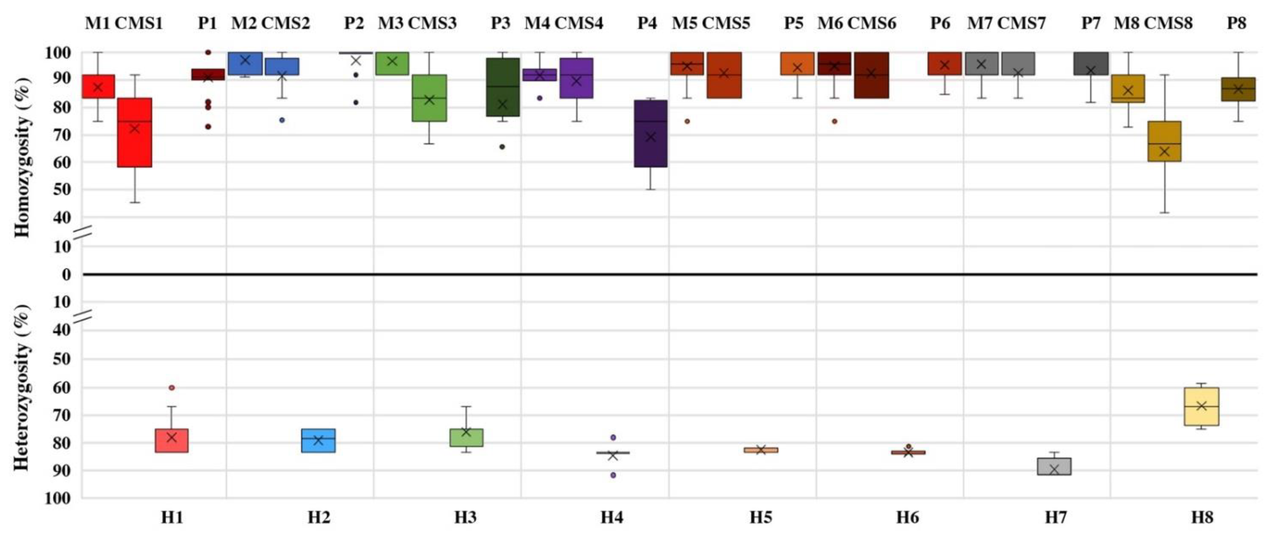
3.2. Genetic Stability of Parental Lines and Distinctiveness of F1 Hybrids

In the constitution of F1 hybrids, the only possibility to sexually propagate the CMS seed plant is through the exploitation of an isogenic fertile ideotype known as a maintainer. To keep the seed plants (and, therefore, the resulting hybrids) uniform and stable over several generations, it is of crucial importance that 1) the maintainer line is, in turn, genetically uniform and 2) the CMS seed plants are produced exclusively by crossing CMS seed plants × isogenic fertile maintainers. For this reason, the same statistics calculated singularly for each line were also calculated for seven groups, each including the maintainer and the related CMS line of each population (Table 4).
Within male-sterile/maintainer groups (CMS-M), the number of polymorphic loci (npl) ranged from 6 to 11, and the number of observed alleles (na) ranged between 1.58 and 2.58. Notably, the number of effective alleles (ne), ranging from 1.07 to 1.39, was consistently lower than the number of observed alleles, demonstrating a high uniformity (i.e., high genetic similarity) within each CMS-M cluster. The high uniformity of most of the CMS-M groups along with the robust differentiation from each other was also evident by comparing the within and among GS estimates (on average 98% and 79%, respectively) and by relating the gene flow (Nm) estimates calculated within and among the CMS-M groups (higher than 1 in the first case and on average 0.05 in the second). In both cases, the low GS values among the CMS-M groups and the total absence of gene flow among them demonstrated the clear differentiation of each CMS-M and the lack of crossings between maternal lines of different populations [25]. Moreover, within-population genetic variability (HS) was found to be lower than 0.10 in seven of the eight groups analyzed in this study (exception made for CMS8-M8, where HS = 0.23), thus demonstrating the high genetic uniformity of the maternal lines in these populations, whereas total genetic differentiation (HT = 0.71) demonstrated the extent of their genetic distinctiveness.
Another aspect to consider when constituting and maintaining a CMS-M group is the degree of homozygosity. The aim is to develop a highly homozygous seed plant to be crossed with a dissimilar and highly homozygous pollinator (P) line. The estimate of the observed homozygosity (Ho) for each CMS-M group provided promising results, with values between 0.74 and 0.95. Specifically, all the CMS-M groups had Ho values higher than 90%, except for CMS1-M1, CMS8-M8 and CMS3-M3, in which additional cycles of siblings are suggested to increase the uniformity of the resulting hybrids.
The high levels of uniformity and homozygosity of each P line are shown in Table 3. In addition, a certain degree of distinctiveness among the pollinator lines was observed, ranging from 69.3% (P4 vs. P7) to 95.8% (P5 vs. P6) (Figure 2). Thus, we hypothesized that there is a genetic relationship among the most similar P lines used in these breeding populations (e.g., P5 vs. P6), putatively derived from common ancestors.

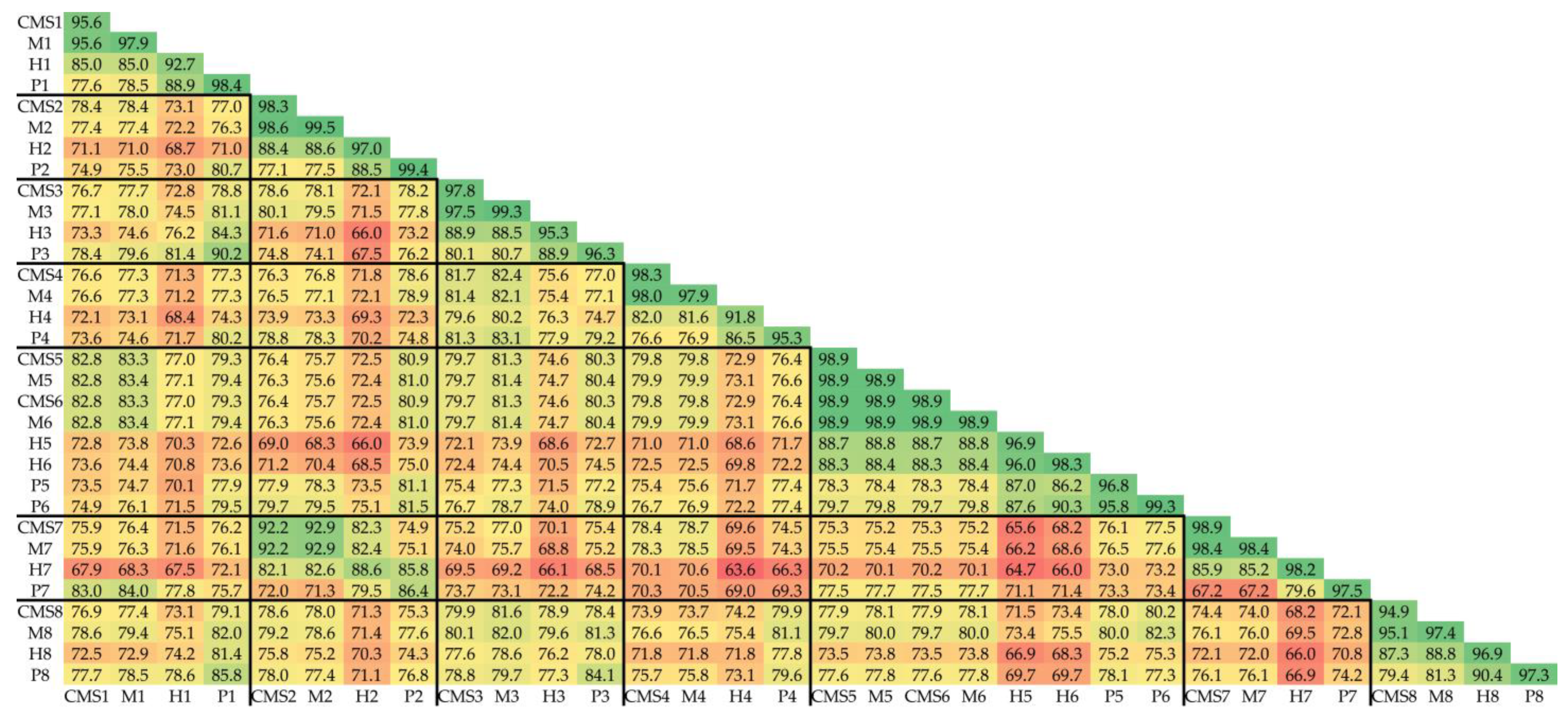
3.3. Genetic Dissimilarity among Parental Lines and Heterozygosity of F1 Hybrids

The GS was also calculated between parental lines (P and CMS). It is important for the GS between CMS and P lines to be as low as possible to maximize the heterotic effect and to obtain highly heterozygous F1 hybrids. The GS in the present study ranged from 67.2% (CMS7 vs. P7) to 80.1% (CMS3 vs. P3, Figure 2). Plotting and organizing the population data based on the increment of hybrid heterozygosity (Figure 3) showed how the hybrids (e.g., H3) exhibiting lower heterozygosity values (yellow area) resulted from highly similar parental lines (e.g., CMS3 and P3; green dashed lines). Conversely, highly dissimilar parental lines produced F1 hybrids characterized by high heterozygosity. In terms of uniformity, Figure 3 clearly demonstrates how the genetic similarity of the parental lines (blue and orange bars) affected the uniformity of the resulting offspring (gray bar). The parental lines with low uniformity values gave rise to low uniform hybrid populations, especially if the parents were characterized by suboptimal homozygosity values (POP1, POP3 and POP8). In POP7, in which CMS and P lines were highly uniform and highly dissimilar (67.2%), the H line resulted in the most heterozygous hybrid population, and one of the most uniform, despite the homozygosity of its pollinator being among the lowest (Ho of P7 = 10.4%). A possible explanation for this could be the small number of hybrids and pollinators analyzed for POP7, resulting in a lack of representativeness. Nevertheless, the results obtained in the other analyzed populations showed a trend for the latter to originate uniform and heterozygous hybrids in relation to the uniformity, genetic dissimilarity and homozygosity of the parental lines.

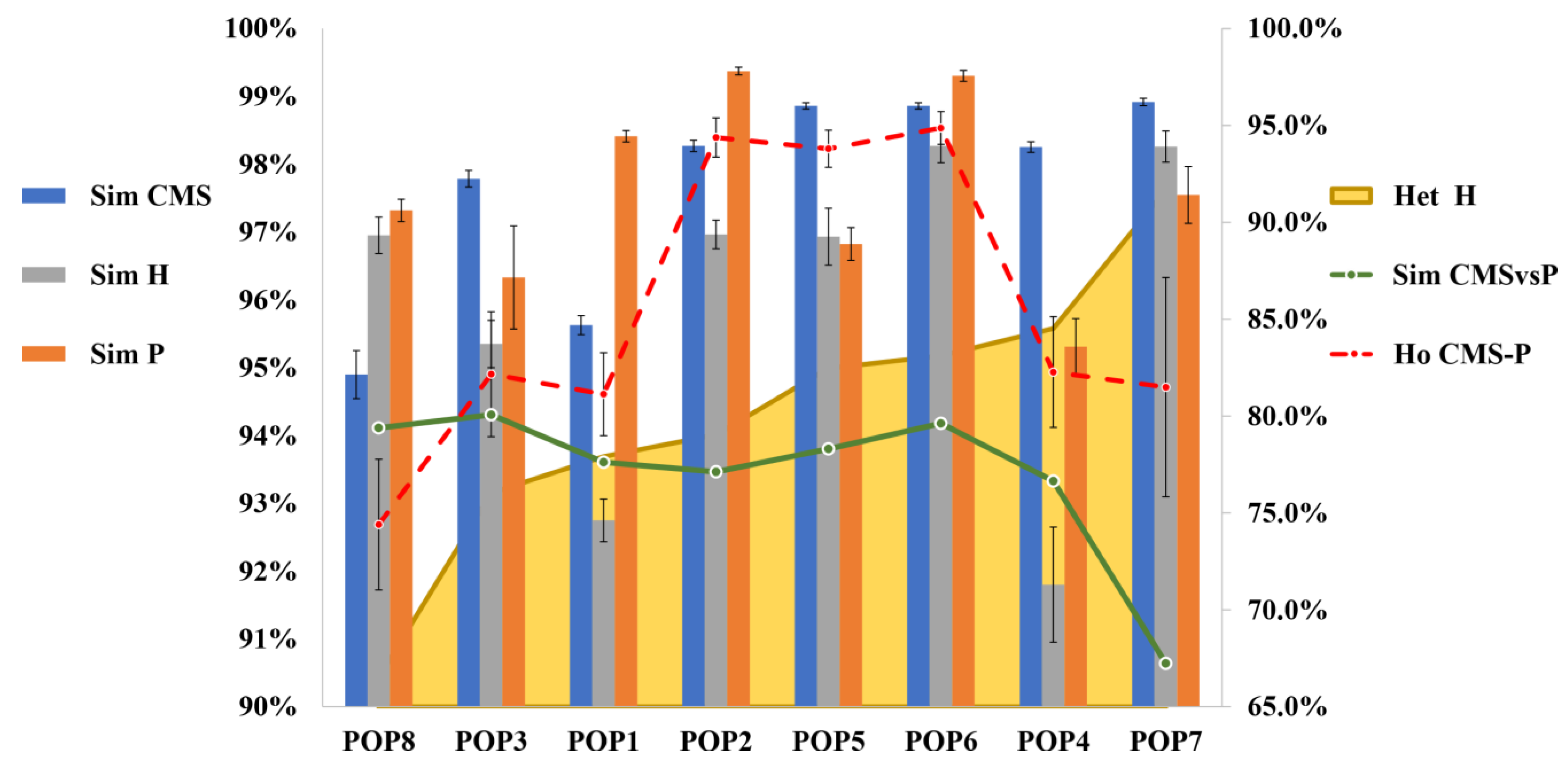
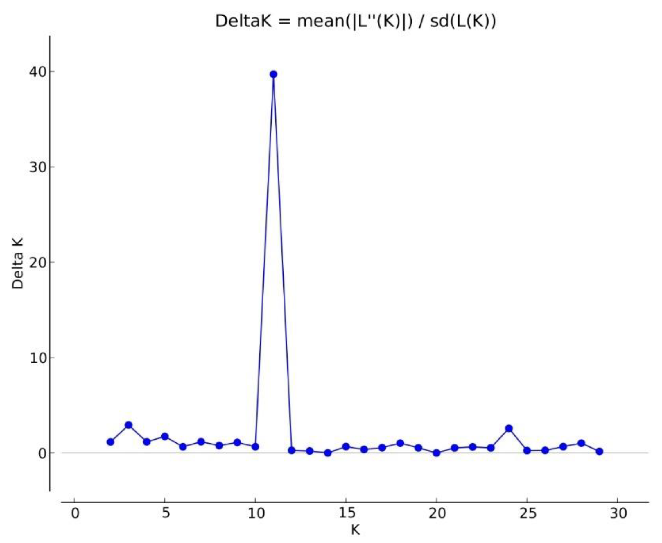
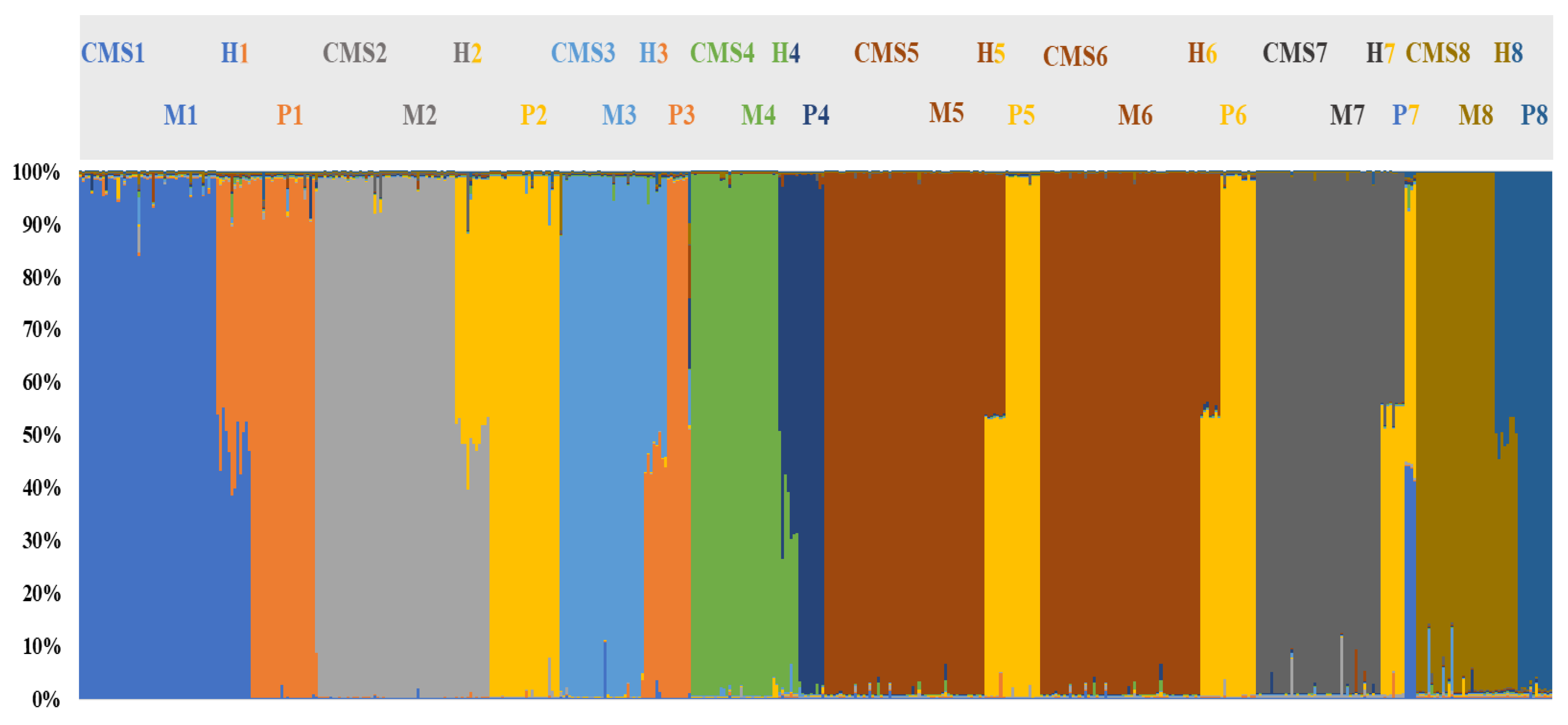
3.4. Genetic Structure of the Core Collection and Genetic Distinctiveness of Breeding Stocks

Following the hypothesis of putative relationships between several breeding lines belonging to different populations, the genetic structure of the fennel core collection was investigated. Using STRUCTURE software [22], 11 clusters were identified that grouped samples in agreement with the breeding line to which they belonged (ΔK = 39.72) (Figure 4 and Figure 5). Specifically, each of the seven CMS-M groups (populations 5 and 6 shared the same maternal lines) was represented by a specific cluster, showing an average membership percentage of 97.6%. According to the GS, and the within (HS) and total (HT) genetic differentiation estimates, these findings confirmed the distinctiveness of each CMS-M group.
The pollinator lines were all represented by four ancestors (different from the seven observed for the CMS-M groups) as follows: P1 and P3 (GS = 90.2%) were ascribed to the same cluster (colored in orange in Figure 5); P2 was grouped with P5 and P6 (average GS = 81.3%) (colored in yellow in Figure 5); and P4 and P8 constituted two separate clusters. Additionally, all samples scored membership values to their respective cluster, consistently higher than 95%, with few exceptions. A separate case was represented by P7, from which the results were (~40%/60%) admixed between P2–P5–P6 and the CMS1–M1 cluster. This finding, in addition to the suboptimal homozygosity and the abnormal gene flow values observed for P7, corroborated the hypothesis that this line is the result of a recent crossing between a maintainer (M1) and a pollinator line (P2, P3 or P6).
Finally, the memberships of the F1 hybrid lines consistently showed memberships of ~50%/50% to the respective maternal and paternal clusters, thus demonstrating the reliability of the clustering method. Thus, the results obtained from the genetic structure reconstruction agreed with the genetic variability results described in Table 3.

4. Conclusions

The genotyping analysis of the core collection of fennel breeding stocks described in this work, along with its genetic descriptive statistics calculation and its genetic structure reconstruction, not only determined the reliability of the method proposed based on microsatellite markers but also provided a suitable molecular approach for plant variety traceability and post-breeding controls. The obtained results discriminated or clustered plant samples depending on the breeding line to which they belonged and identified unsuitable parental genotypes (e.g., P7), even though the hybrid progenies obtained in the breeding program were genetically uniform and highly heterozygous. The overall results highlighted the impossibility of the SSR marker panel used in this study to univocally discriminate pollinator lines, thus suggesting the necessity of increasing the number of SSR markers for the identification of closely related inbreds. Additionally, a certain correlation between the uniformity and heterozygosity of the F1 hybrids with the respective parental stability and dissimilarity, i.e., within-population genetic similarity and between-population diversity, was observed, demonstrating the suitability of molecular markers in helping breeders to partially predict the genetic background of F1 hybrids when planning two-way crosses.
In conclusion, the genotyping method described in the present study can be used for different applications related to the development of new fennel varieties and to the assessment of their genetic identity for genetic traceability and legal protection purposes. Further implementations will be performed in the future to investigate other informative SSR marker loci to be used for marker-assisted breeding (MAB) aims or for assessing distinctiveness, uniformity and stability (DUS) of new plant varieties.

Supplementary Materials

The following are available online at https://0-www-mdpi-com.brum.beds.ac.uk/article/10.3390/agronomy12030542/s1, Table S1: Dataset containing the raw data of the 451 genotypes analyzed with 12 SSR marker loci.

Author Contributions

Conceptualization, F.S. and G.B.; methodology, F.S. and F.P.; validation, F.S. and F.P.; formal analysis, F.S.; investigation, F.S. and F.P.; resources, G.B.; data curation, F.S. and F.P.; writing—original draft preparation, F.S. and F.P; writing—review and editing, F.S., F.P. and G.B.; visualization, F.S and F.P.; supervision, G.B.; project administration, G.B.; funding acquisition, G.B. All authors have read and agreed to the published version of the manuscript.

Funding

This research received no external funding.

Institutional Review Board Statement

Not applicable.

Informed Consent Statement

Not applicable.

Conflicts of Interest

The authors declare no conflict of interest.

References

  1. Badgujar, S.B.; Patel, V.V.; Bandivdekar, A.H. Foeniculum vulgare Mill: A review of its botany, phytochemistry, pharmacology, contemporary application, and toxicology. BioMed Res. Int. 2014, 2014, 842674. [Google Scholar] [CrossRef] [PubMed] [Green Version]
  2. Diaz-Maroto, M.C.; Perez-Coello, M.S.; Esteban, J.; Sanz, J. Comparison of the volatile composition of wild fennel samples (Foeniculum vulgare Mill.) from central Spain. J. Agric. Food Chem. 2006, 54, 6814–6818. [Google Scholar] [CrossRef] [PubMed]
  3. Palumbo, F.; Vannozzi, A.; Vitulo, N.; Lucchin, M.; Barcaccia, G. The leaf transcriptome of fennel (Foeniculum vulgare Mill.) enables characterization of the t-anethole pathway and the discovery of microsatellites and single-nucleotide variants. Sci. Rep. 2018, 8, 10459. [Google Scholar] [CrossRef] [PubMed]
  4. Senatore, F.; Oliviero, F.; Scandolera, E.; Taglialatela-Scafati, O.; Roscigno, G.; Zaccardelli, M.; De Falco, E. Chemical composition, antimicrobial and antioxidant activities of anethole-rich oil from leaves of selected varieties of fennel [Foeniculum vulgare Mill. ssp. vulgare var. azoricum (Mill.) Thell]. Fitoterapia 2013, 90, 214–219. [Google Scholar] [CrossRef]
  5. Tognolini, M.; Ballabeni, V.; Bertoni, S.; Bruni, R.; Impicciatore, M.; Barocelli, E. Protective effect of Foeniculum vulgare essential oil and anethole in an experimental model of thrombosis. Pharm. Res. 2007, 56, 254–260. [Google Scholar] [CrossRef]
  6. FAO. FAOstat. Available online: http://www.fao.org/home/en (accessed on 22 December 2021).
  7. Palumbo, F.; Vannozzi, A.; Barcaccia, G. Impact of Genomic and Transcriptomic Resources on Apiaceae Crop Breeding Strategies. Int. J. Mol. Sci. 2021, 22, 9713. [Google Scholar] [CrossRef] [PubMed]
  8. Koul, P.; Sharma, N.; Koul, A.K. Pollination Biology of Apiaceae. Curr. Sci. 1993, 65, 219–222. [Google Scholar]
  9. Palumbo, F.; Vitulo, N.; Vannozzi, A.; Magon, G.; Barcaccia, G. The Mitochondrial Genome Assembly of Fennel (Foeniculum vulgare) Reveals Two Different atp6 Gene Sequences in Cytoplasmic Male Sterile Accessions. Int. J. Mol. Sci. 2020, 21, 4664. [Google Scholar] [CrossRef]
  10. Pank, F. Three approaches to the development of high performance cultivars considering the differing biological background of the starting material. In Proceedings of the International Conference on Medicinal and Aromatic Plants. Possibilities and Limitations of Medicinal and Aromatic Plant, Budapest, Hungary, 8–11 July 2001; pp. 129–137. [Google Scholar]
  11. Palumbo, F.; Galla, G.; Vitulo, N.; Barcaccia, G. First draft genome sequencing of fennel (Foeniculum vulgare Mill.): Identification of simple sequence repeats and their application in marker-assisted breeding. Mol. Breed. 2018, 38, 122. [Google Scholar] [CrossRef]
  12. Schuelke, M. An economic method for the fluorescent labeling of PCR fragments. Nat. Biotechnol. 2000, 18, 233–234. [Google Scholar] [CrossRef] [PubMed]
  13. Palumbo, F.; Galla, G.; Martinez-Bello, L.; Barcaccia, G. Venetian Local Corn (Zea mays L.) Germplasm: Disclosing the Genetic Anatomy of Old Landraces Suited for Typical Cornmeal Mush Production. Diversity 2017, 9, 15. [Google Scholar] [CrossRef] [Green Version]
  14. Palumbo, F.; Galla, G.; Barcaccia, G. Developing a Molecular Identification Assay of Old Landraces for the Genetic Authentication of Typical Agro-Food Products: The Case Study of the Barley ’Agordino’. Food Technol. Biotechnol. 2017, 55, 29–39. [Google Scholar] [CrossRef]
  15. Yeh, F.C.; Yang, R.C.; Boyle, T.B.J.; Ye, Z.H.; Mao, J.X. POPGENE, The User-Friendly Shareware for Population Genetic Analysis; University of Alberta: Edmonton, AB, Canada, 1998; Volume 10, pp. 295–301. [Google Scholar]
  16. Serrote, C.M.L.; Reiniger, L.R.S.; Silva, K.B.; Rabaiolli, S.M.D.S.; Stefanel, C.M.; Lemos, S.C.M.; Silveira, R.L.R.; Buuron, S.K.; Dos Santos, R.S.M.; Moro, S.C. Determining the Polymorphism Information Content of a molecular marker. Gene 2020, 726, 144175. [Google Scholar] [CrossRef]
  17. Kimura, M. Population Genetics, Molecular Evolution, and the Neutral Theory: Selected Papers; University of Chicago Press: Chicago, IL, USA, 1994. [Google Scholar]
  18. Nei, M. Molecular Evolutionary Genetics; Columbia University Press: New York, NY, USA, 1987. [Google Scholar]
  19. Mcdermott, J.M.; Mcdonald, B.A. Gene Flow in Plant Pathosystems. Annu. Rev. Phytopathol. 1993, 31, 353–373. [Google Scholar] [CrossRef]
  20. Barcaccia, G.; Lucchin, M.; Parrini, P. Characterization of a flint maize (Zea mays var. indurata) Italian landrace, II. Genetic diversity and relatedness assessed by SSR and Inter-SSR molecular markers. Genet. Resour. Crop. Evol. 2003, 50, 253–271. [Google Scholar] [CrossRef]
  21. Rohlf, F.J. NTSYS-pc: Numerical Taxonomy and Multivariate Analysis System Version 2.1: Owner Manual; Exeter Publishing: Setauket, NY, USA, 2000. [Google Scholar]
  22. Pritchard, J.K.; Stephens, M.; Donnelly, P. Inference of population structure using multilocus genotype data. Genetics 2000, 155, 945–959. [Google Scholar] [CrossRef]
  23. Earl, D.A.; Vonholdt, B.M. STRUCTURE HARVESTER: A website and program for visualizing STRUCTURE output and implementing the Evanno method. Conserv. Genet. Resour. 2011, 4, 359–361. [Google Scholar] [CrossRef]
  24. Botstein, D.; White, R.L.; Skolnick, M.; Davis, R.W. Construction of a genetic linkage map in man using restriction fragment length polymorphisms. Am. J. Hum. Genet. 1980, 32, 314–331. [Google Scholar]
  25. Mitton, J.B. Gene Flow. In Brenner’s Encyclopedia of Genetics, 2nd ed.; Maloy, S., Hughes, K., Eds.; Academic Press: Cambridge, MA, USA, 2013; pp. 192–196. [Google Scholar]
Figure 1. Box plot of the median observed homozygosity (top) and observed heterozygosity (bottom) related to, respectively, parental lines (M, maintainer; cytoplasmic male-sterile, CMS; P, pollen donor) and F1 hybrid (H) offspring for each fennel breeding scheme. Each population is labeled with different colors (the CMS and M lines of each variety have the same color tone whereas P lines are represented by a darker color and H hybrids show a lighter color). The second and third quartiles are marked inside the square and are divided by a bar (median). The cross (×) within each box represents the mean value. Dots show outlier samples.
Agronomy 12 00542 g001
Figure 2. Average genetic similarity percentages (GS%) calculated within and among each population using Rohlf’s simple matching coefficient. Variance values for each pairwise comparison between lines and within lines were also computed, resulting in <0.5%.
Agronomy 12 00542 g002
Figure 3. Graphical representation of the genetic similarity (Sim) calculated within the CMS (blue bar), H (gray bar) and P (orange bar) lines of each population (vertical scale on the left) as well as the H line heterozygosity (yellow area), genetic similarity among the CMS and P lines (green dashed line) and their average homozygosity (red dashed line) (vertical scale on the right).
Agronomy 12 00542 g003
Figure 4. ΔK estimation from STUCTURE Harvester web software elaboration of the STRUCTURE software results. The most probable value of K was equal to 11.
Agronomy 12 00542 g004
Figure 5. Histogram representing the membership of each sample to one of the 11 identified clusters. The names of each line are reported above bars and are labeled with the same color of the respective cluster.
Agronomy 12 00542 g005
Table 1. List of SSR markers reporting locus name, forward and reverse primer sequences (5′ to 3′), microsatellite motif, minimum and maximum size (bp) and anchor type [11].
Locus
Name
Primer ForwardPrimer ReverseMotifMin SizeMax SizeAnchor
FV_2CAAAGAATGGAAAACATGCTGCAAAGAATGGAAAACATGCTGCAA129152PAN1
FV_6TATGTTCTCAGATTCGGGTTATATGTTCTCAGATTCGGGTTATC214226M13
FV_253TTGTAGAGATACAGGGTCGAATTGTAGAGATACAGGGTCGAATC196252PAN1
FV_9919AGTAAAGGCATAATCTGTTGGTGGAGTAAAGGCATAATCTGTTGGTGGGT231248PAN3
FV_11537TTCATGTATCAACTACGCACACTTCATGTATCAACTACGCACACAG152166M13
FV_15981CTAGCGTTTCCATCTCGTCTCCTAGCGTTTCCATCTCGTCTCTC235245PAN1
FV_18902GTTTGAACTCGAATGACCACCTGTTTGAACTCGAATGACCACCTTC410424PAN2
FV_179837ATTCACCATGACATCACCTCATTCACCATGACATCACCTCTC320336M13
FV_217218ACAAACGTACCTCTGTACGAAACAAACGTACCTCTGTACGAAAG345360M13
FV_217225AAAGAATGGAGAGAAGAATGGAAAGAATGGAGAGAAGAATGGAG309344PAN1
FV_290063TGATTTCTCAAAGGCATTCTATGATTTCTCAAAGGCATTCTAGA294324PAN3
FV_290202AGGGCTGAGATTAGTTTCTAGTTAGGGCTGAGATTAGTTTCTAGTTTA139210PAN2
Table 2. Descriptive statistics of SSR markers reporting the polymorphic information content (PIC), number of marker alleles per locus and the highest marker allele frequency observed per locus (PIC coefficients are calculated as Nei’s diversity, in agreement with Palumbo and Serrote [11,16]).
Locus NamePICN.
Alleles
Highest Allele Frequency
FV_20.7370.366
FV_60.6570.514
FV_2530.86130.234
FV_99190.6950.343
FV_115370.8060.290
FV_159810.6350.472
FV_189020.8080.279
FV_1798370.7990.346
FV_2172180.7580.405
FV_2172250.85110.194
FV_2900630.7780.288
FV_2902020.89150.186
Mean0.778.50.326
Table 3. Descriptive statistics for all SSR loci, including number of individuals (N), number (npl) of polymorphic loci, percentage (%pl) of polymorphic loci, mean number of observed (na) alleles per locus, mean number of effective (ne) alleles per locus, observed (Ho) homozygosity, expected (He) homozygosity, Nei’s genetic diversity (H) and gene flow estimates (Nm).
Population IDNnpl%plnaneHoHeHNm
CMS1241083.3%2.331.390.720.770.230.32
CMS224433.3%1.671.110.910.920.080.33
CMS316758.3%1.581.210.830.860.130.44
CMS416541.7%1.421.150.900.910.090.33
CMS527433.3%1.331.100.940.940.060.24
CMS627433.3%1.331.100.940.940.060.24
CMS724541.7%1.501.090.930.940.060.34
CMS8141191.7%2.251.470.640.720.280.43
Average CMS20.76.654.8%1.731.220.840.870.130.35
M123758.3%1.751.160.870.890.110.32
M224433.3%1.331.030.970.970.030.14
M313433.3%1.331.030.970.970.030.28
M414325.0%1.421.190.920.910.090.21
M528541.7%1.421.100.950.950.050.23
M628541.7%1.421.100.950.950.050.23
M719541.7%1.751.090.930.930.070.32
M813541.7%1.501.210.860.870.130.30
Average M19.14.739.3%1.501.120.920.930.070.26
P122866.7%1.831.180.920.880.110.34
P224541.7%1.501.110.980.920.070.05
P38975.0%2.001.230.810.840.150.39
P49866.7%1.901.490.690.750.240.42
P512325.0%1.501.270.920.870.130.10
P612216.7%1.171.050.960.960.030.39
P741191.7%2.081.980.100.460.474.78
P812650.0%1.501.230.860.860.130.18
Average P11.66.352.4%1.671.340.760.810.180.90
H1121083.3%2.752.160.220.500.480.98
H2121191.7%2.251.910.210.550.432.35
H381191.7%2.421.940.240.540.441.70
H471191.7%2.752.310.160.440.521.08
H571083.3%2.172.010.170.510.451.56
H671083.3%2.001.930.170.530.433.51
H7812100.0%2.171.990.060.480.495.00
H88975.0%1.921.790.320.590.380.73
Average H8.110.688.1%2.241.980.190.520.452.28
Overall Mean 7.259.7%1.821.43
Among overall451 0.780.230.770.09
Table 4. Descriptive statistics for all SSR loci for CMS-M groups. The number of individuals (N), number (npl) of polymorphic loci, percentage (%pl) of polymorphic loci, mean number of observed (na) alleles per locus, mean number of effective (ne) alleles per locus, total (HT) genetic variability, within (HS) genetic variability, observed (Ho) homozygosity, expected (He) homozygosity, Rohlf’s simple matching genetic similarity (GS) coefficient and gene flow estimates (Nm). The mean values within population (Mean CMS-M) and the mean values calculated considering all the possible pairwise comparisons among the CMS-M groups were estimated.
Population IDNnpl%plnaneHTHSHoHeGSNm
CMS1_M1471083.3%2.581.28 0.190.800.810.962.38
CMS2_M248650.0%1.831.07 0.060.940.940.993.53
CMS3_M3291083.3%1.921.13 0.100.890.900.981.78
CMS4_M430650.0%1.671.17 0.100.910.900.988.34
CMS5_M555758.3%1.581.10 0.060.950.950.9969.19
CMS6_M655758.3%1.581.10 0.060.950.950.9969.19
CMS7_M743758.3%1.921.09 0.070.930.940.984.39
CMS8_M8271191.7%2.421.39 0.230.740.770.951.98
Mean CMS-M2798.167.9%1.991.180.71
St. Dev. 2.117.6%2.681.15
Among CMS-M 0.890.290.790.05
St. Dev. 0.070.070.02
Publisher’s Note: MDPI stays neutral with regard to jurisdictional claims in published maps and institutional affiliations.

