Effects of Agricultural Management Practices on the Temporal Variability of Soil Temperature under Different Crop Rotations in Bad Lauchstaedt-Germany

Abstract

To investigate the effects of management practices on the dynamics of soil temperature, during 2014–2017, a field experiment was carried out in Bad Lauchstaedt, Germany. In this study, four management systems are compared for determining management-induced changes in soil temperature at different depths: (i) conventional tillage (T_C) with the standard rate of N fertilizer (P1N1), (ii) conventional tillage with the half-standard rate of N fertilizer (P1N0), (iii) reduced tillage (T_R) with the standard rate of N fertilizer (P0N1), and iv) reduced tillage with the half-standard rate of N fertilizer (P0N0). Temporal analysis of soil temperature is assessed to examine data observed at a specific time to achieve a better understanding of the soil temperature dynamic that occurs at different time scales. The results showed that the soil temperature has decreasing amplitudes and increasing phase shifts with increasing soil depth, i.e., the deeper the measurement depth, the smoother the soil temperature changes cycle and the smaller the variability. Results showed that the diurnal temperature variation is found up to 45 cm depth of soil whereas annual temperature variation is up to a depth of 180 cm. The results, moreover, revealed that soil temperature dynamic was affected by tillage systems and fertilization and a time lag is observed between the temperature fluctuations at the surface and deeper layers, due to induced management effects on plant cover, residues, and soil properties. Although higher soil temperature at the sowing stage under TR is contributed to higher amounts of surface crop residues in crop rotations, the effect of residues on soil temperature variation reduces with an increase in percent plant cover and shading of soil, which happens in the last stage of plant growth. At the last stage of crop development regardless of tillage systems, applying more N fertilization increased crop yield, resulting in cooling soil temperature.

1. Introduction

Soil Temperature (T_s), as one of the important factors, plays an essential role in climatology, agriculture, ecosystems, hydrology, and the environment and is the most fundamental component of the Earth’s surface energy budget by regulating the heat energy exchange between the land surface and the atmosphere [1]. The factors that affect the amount of heat supplied at the soil profile include not only climatic variability such as diurnal air temperature (T_air) oscillations, and solar radiation, but also soil surface attributes such as vegetative cover, organic matter content, evaporation, and soil color as well as disturbances due to management practices [2]. Soil management activities affect T_s mostly by altering the reflection coefficient, thereby changing the net radiation at the soil surface.

Soil tillage as a common agricultural management practice strongly affects T_s and soil moisture in the near-surface unsaturated soil zone that plays as an interface between the subsurface and the low atmosphere boundary [3]. Soil tillage systems control hydrological cycles and energy balance and alter soil water use efficiency, soil fertility, air and heat flow by inducing some changes in soil properties such as shape, size, and continuity of soil pores and soil water content [4]. Conventional tillage (T_C) is mainly plowed up to 20–25 cm soil depth, which causes a decrease in soil bulk density, and an increase in soil porosity thereby may have a positive impact on plant growth. However, T_C adversely affects soil structure by reducing soil aggregation, and can also create hardpan by compaction from repeated plowing, leading to an increased risk of erosion and nutrient loss as well as a decrease in water infiltration into deeper soil layers [5]. To conserve natural resources, and mitigate the potential disadvantages of T_C on sustainable agriculture, there is a greater interest in using reduced tillage (T_R). T_R together with soil surface cover and rotation can not only increase aggregate stability and bulk density but also decrease soil mechanical impedance and water evaporation compared to T_C and then affect soil temperature in crop lands [6].

Another major challenge ahead is to apply fertilizers in a way that maintains soil sustainability while ensuring adequate food production with minimal environmental impacts. Different fertilizer management schemes may affect T_s through effects on crop yield. The shade provided by a dense shrub cover during the growing season might reduce T_s [7]. Although excessive fertilizer input does not lead to a further increase in crop yield, it could increase the risk of environmental pollution, such as N and P leaching into groundwater and N emissions into the atmosphere [8]. Recently, strategies have been proposed to reduce the fertilizer application rate to a sufficient level that might meet the needs of a crop [9].

Despite wide research on the effect of management on T_s changes, there is insufficient investigation on the interaction effects of tillage and N fertilization on T_s behavior in shallow and deep soil layers at different temporal courses. The current study was conducted in the framework of a field experiment in a Bad Lauchstaedt-Germany, to explore the interaction effects of soil tillage and fertilization on T_s variation in different soil depths. In this study, T_s of the various soil layers were monitored to more realistically describe the temperature changes at different soil layers and analyze management-induced changes from various perspectives. We hypothesized that soil management practices significantly influence T_s fluctuation. Applying statistical time series analysis of T_s provides advantages for a better understanding of T_s responses to management practices. Therefore, quantifying the effect of management systems on T_s can explain some of the differences in plant growth and development in applied management systems.

2. Material and Method

2.1. Study Site and Soil Information

The study site is part of the field research station of the Helmholtz-Centre for Environmental Research in Bad Lauchstaedt, Sachsen-Anhalt, Germany (51°24′ N, 11°53′ E and 118 m above the sea level). The investigations were carried out during the four years 2014–2017. The meteorological data were available for the investigation period from a weather station that was in operation on the field research station. The annual mean precipitation was 434 mm (2014–2017), 63% of which occurs between March and August. The mean annual temperature at the site was 10 °C. The region has four distinct seasons: spring (March (60th day of the year)–May (151th day of the year)), summer (June (152th day of the year)–August (243th of the year)), autumn (September (244th day of the year)–November (334th day of the year)), and winter (December (335th day of the year)–February (59th day of the year)). The region has flat terrain topography with uniform fertility. The soil type in this experiment is Haplic Chernozem (FAO) (USDA: Mollisol), consisting of 21.0% clay, 67.8% silt, and 11.2% sand and are dark brown to black in color, due to their enrichment of high-quality humus [10]. Groundwater level in studied site is deeper than 2 m. Site conditions were described in detail by Alterman et al. [10]. Before setting up the field experiments, soil samples were collected for chemical and physical characterization, presented in

Table 1. Some soil parameters in Bad Lauchstaedt at different soil depths.

Soil Parameters	Soil Depth (cm)
	5	45	90	180
Organic carbon (%)	2.1	1	0.2	0.1
Bulk density (g cm−3)	1.36	1.38	1.49	1.79
Particle density (g cm−3)	2.65	2.65	2.67	2.67
Field capacity (Vol. %)	32.9	30.0	28.5	18.9
Permanent wilting point (Vol. %)	16.9	18.1	9.1	12.9
Saturated hydraulic conductivity (mm d−1)	355.0	355.0	355.0	353.0

.

2.2. Experimental Design and Crop Management

In this study, two management factors of soil tillage and N fertilization were investigated in a non-randomized experiment. The trial was laid out in a split plot design with two tillage systems, i.e., (1) conventional tillage with a plowing depth around 20–30 cm (P1) and (2) reduced tillage with plowing depth around 5–10 cm (P0) and two N fertilizer level, i.e., (1) conventional N-fertilizer: standard rate of mineral fertilizer treatment (100 kg ha⁻¹) that reflects the practice of local (N1); (2) reduced N-fertilizer: half-standard rate (50 kg ha⁻¹) of mineral fertilizer (N0). The dimension of plots were 20 m × 22 m which were planted with spring rape (Brassica napus), winter wheat (Triticum aestivum), winter barley (Hordeum vulgare), and winter rape (Brassica napus) as a typical regional crop rotation (

Table 2. Crop rotation date in the studied period in four studied plots.

Crops	Sowing Date	Harvest Date
Spring Rape	March 2014	August 2014
Winter Wheat	October 2014	July 2015
Winter Barley	September 2015	Jun 2016
Winter Rape	September 2016	April 2017
Spring Rape	April 2017	August 2017

). A schematic diagram showing the experimental design is presented in

Table 3. Field experimental design of tillage and N-fertilizer applications.

Plot Design		Management Factor 2 (N-Fertilization)
		Conventional	Reduced
Management factor 1 (Tillage)	Conventional	P1N1	P1N0
	Reduced	P0N1	P0N0

. Total mineral fertilizer was applied in spring. For all plots, the straw of the previous crop was uniformly broadcasted into the top soil before plowing the soil.

2.3. Soil Temperature

T_s monitoring commenced in 2014 and ended in 2017. On each studied plot three sensors were horizontally installed at 5, 45, 90, and 180 cm soil depths. T_s were automatically recorded every 10 min by PT1000 sensors (Platinum resistance thermometers) which provide excellent accuracy over a wide temperature range. The data integrity is considered satisfactory (i.e., the amount of missing data annually is <5%).

For the characterization of the T_s, we used hourly averages for daily fluctuation and daily averages for monthly and annual fluctuation. A very large quantity of temperature measurements was obtained in this work. To reduce the quantity of data and to emphasize the major effects, two statistical operations were carried out.

As the study duration could have a significant impact on the variation of T_s, so recorded data during the crop growing season were assessed into the hottest and coldest days of each year. Furthermore, two important days (sowing and a day before harvest) were selected to present the effects of different management conditions at various soil depths. Although these two days could be exceptional, we have checked these days represent the typical condition for a longer interval.

To analyze the variation of the T_s at 5 cm soil depth at different day times during the whole crop growing season, the T_s at a depth of 5 cm at 00:00 h, 06:00 h, 14:00 h, and 18:00 h every 15 days after sowing (days after sowing-DAS) was determined.

2.4. Data Analysis

Measured T_s curves were fitted by utilizing a sinusoidal function to represent variations of heat transferred to the soil and the depth of T_s penetration. The behavior of T_s was fitted for different soil layers of selected thermal periods using the equation [11]. A simple sine curve could be written:

$$y\left(z,t\right)=A\cdot sin\left(\omega t+\phi z\right)+T_{average}$$

(1)

where y(z,t) is the T_s (°C) at depth z and time t, T_average is the average T_s (°C), A is the amplitude of the soil thermal wave (°C), which provides insight into the temperature fluctuations, ω is the radial frequency (per unit time), that equals to 2π/p and p is the period of temperature fluctuation and is set to 24 h for one day or 365 days for one year denoting the period of the fundamental cycle, φ_z is the phase shift (rad), the delay of T_s changes at soil layers. The model parameters T_average, A, and φ_z were determined using the lm function in R software as shown below [12]:

A general sine curve can be considered and described as a general linear combination of sin and cos to estimate the model by using a linear curve fitting algorithm:

$$y=\alpha \mathit{sin}\left(x\right)+\beta \mathit{cos}\left(x\right)$$

(2)

(α, β) are the parameters of the Equation (2), which consider as a vector and is written in polar coordinates (A, φ),

$$\alpha =A\mathit{cos}\left(\phi \right)$$

(3)

$$\beta =A\mathit{sin}\left(\phi \right)$$

(4)

whence,

$$y=\alpha \mathit{sin}\left(x\right)+\beta \mathit{cos}\left(x\right)=A\mathit{cos}\left(\phi \right)\mathit{sin}\left(x\right)+A\mathit{sin}\left(\phi \right)\mathit{cos}\left(x\right)=A sin\left(x+\phi \right)$$

(5)

$$A=\sqrt{{\alpha }^2+{\beta }^2}$$

(6)

$$\phi =\mathit{arctan}(\frac{\beta }{\alpha })$$

(7)

The phase shift can be also determined in terms of the time period (days), in this study, one rotation takes 365 days, thus

The period is 365 days, i.e., 2π ≙ 356 days, so:

$$365=\frac{2\pi }{\omega }\mathrm{or}\omega =\frac{2\pi }{365}$$

(8)

Now we need to find the phase shift, φ ≙ n days, so:

$$\frac{2\pi }{365\left(d\right)}=\frac{\phi \left(\mathit{rad}\right)}{n\left(d\right)}$$

(9)

$$n=\frac{\phi 365}{2\pi }$$

(10)

If we divide the period of 365 days into 4 subintervals, each subinterval will be 91.25 days long. Therefore, the number of days from an arbitrary starting date (taken as January 1 in this study) to the occurrence of the maximum temperature in a year (days) can be calculated as follow:

$$\mathrm{Time}\mathrm{lag}=n\left(d\right)+91.25\left(d\right)$$

(11)

The coefficient of correlations among air and T_s at various soil depths were determined using Pearson correlation analyses whereas T_air is considered independent and T_s is the dependent variable. This coefficient demonstrates the association between the response ratios of T_s to the T_air during the studied period that creates regression equations through which the T_s is projected corresponding to the T_air.

The data were evaluated to assess differences among treatments by analysis of variance using R statistical software. The T_s of a plot was always taken into account as the mean value of the three sensors. Mean values from treatments were compared based on the least significant difference test (LSD 0.05) if the F-tests were significant at a probability level of 0.05.

3. Results and Discussion

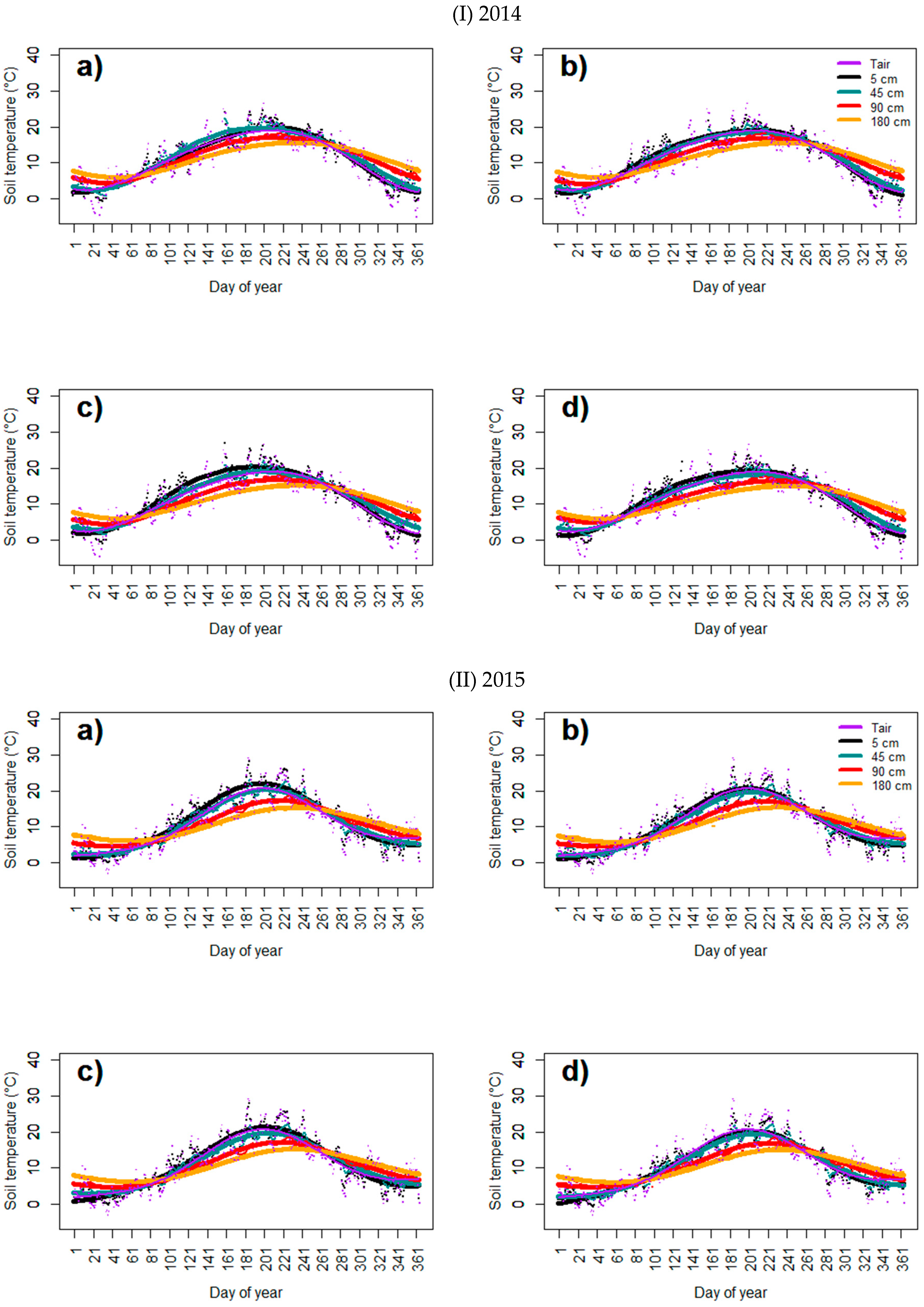
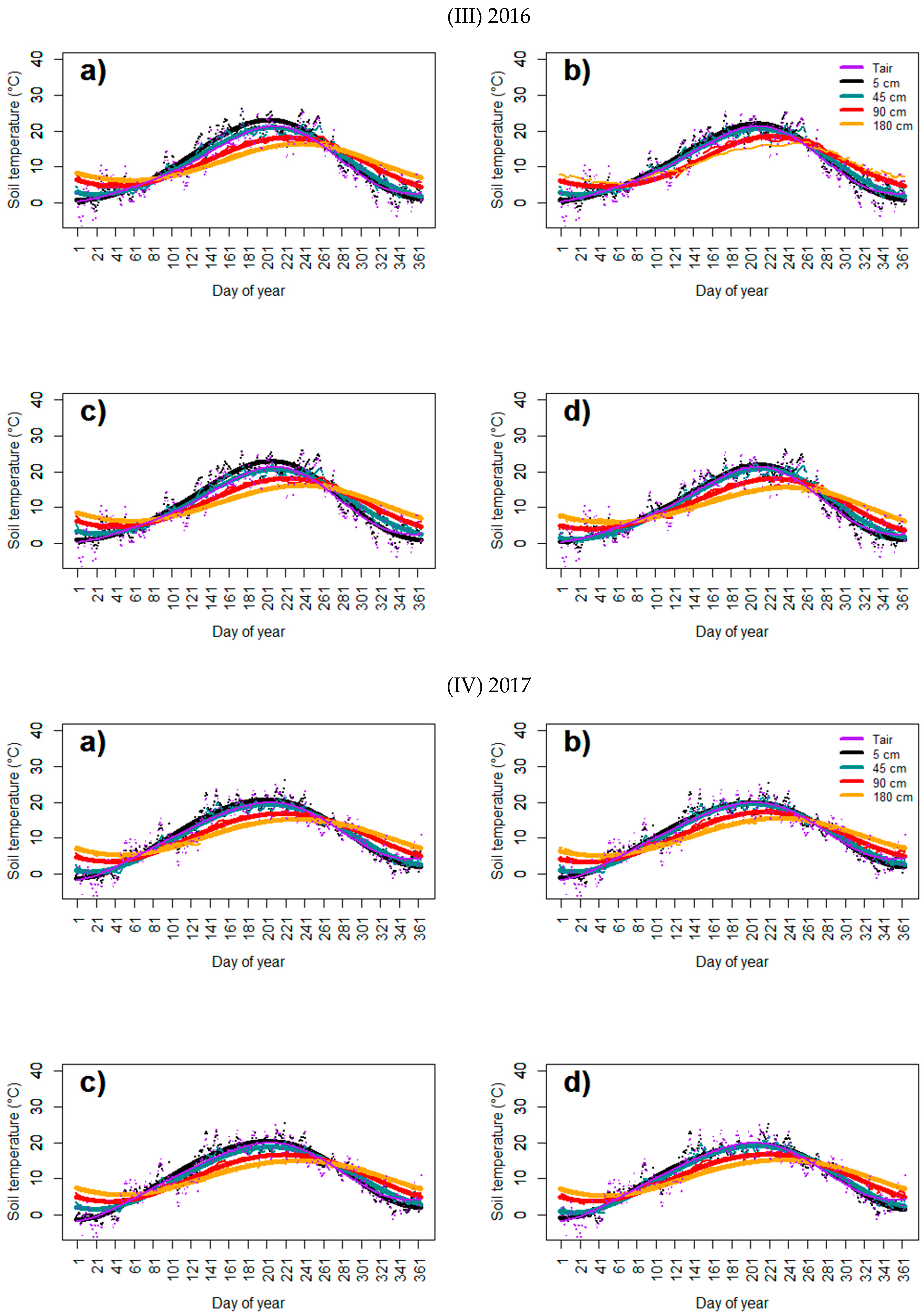
3.1. Information on Soil Temperature Changes in Different Temporal Courses

A sinusoidal wave model was applied under the assumption that the T_s varied in a sinusoidal manner. Fitted soil thermal wave behavior in different soil layers of all treatments during the studied years are shown in Figure 1 aiming to provide an insight into the T_s changes and their relationship with changes in T_air. Figure 1 shows that the temperature of the ground surface at 5 cm remains almost in phase with that of the air and T_air has remained lower than soil surface temperature from 60th day of the year to 274th day of the year (March to October) over studied years. It can be explained that during these months, the surface heating of the atmosphere is greater than the cooling effect [13]. Differences between the monthly average of T_air and at 5 cm depth T_s at P0N0 and P1N0 from 60th day of the year to 274th day of the year (March to October) are more pronounced than P0N1 and P1N1 can be due to more ground cover and shading of soil in plots with the standard rate of fertilizer, and these differences become less in the remaining months (Figure 1). Irrespective of treatment effects, the changes in T_s in warm months showed a tendency to decrease as the depth increased, while in cold months, T_s was higher in subsoils than topsoil. These measurements are similar to the previous studies [4,14,15,16]. Variations of T_s in deep soil layers are much less compared to the upper layers, and lag considerably behind the seasonal variations in comparison with the upper layers; i.e., the maximum or minimum occurs later than the corresponding values at the surface, and a time lag is observed between the temperature fluctuations at the surface and in the deeper layers.

The daily amplitude of T_s at the surface is greater than the daily amplitude of T_air, and T_s decreases in amplitude and increases in phase shift (time offset) with depth (

Table 4. Fitted parameters of the sinusoidal wave of soil temperature variation in the different soil layers under different managements during studied years.

Treatments	Depth (cm)	Amplitude (°C)	Phase Shift (rad)	Phase Shift (day)	Taverage (°C)	Time Lag (day)
		2014
Air		8.4	−1.8	104	11.2	196
P0N0	5	9.5	−1.8	104	11.8	196
	45	8.8	−1.9	110	11.7	202
	90	6.5	−2.1	124	11.4	213
	180	4.8	−2.4	138	11.3	230
P0N1	5	8.8	−1.8	106	11.3	197
	45	8.2	−1.9	111	11.3	203
	90	6.3	−2.1	122	11.2	214
	180	4.7	−2.4	139	11.2	230
P1N0	5	9.5	−1.8	104	11.7	196
	45	8.1	−1.9	111	11.6	202
	90	6.2	−2.2	125	11.3	216
	180	4.5	−2.4	139	11.1	231
P1N1	5	9.0	−1.8	104	11.4	196
	45	8.0	−2.0	113	11.3	204
	90	5.9	−2.2	128	11.3	220
	180	4.5	−2.4	141	11.0	232
		2015
Air		8.0	−1.8	102	10.8	193
P0N0	5	9.4	−1.8	102	11.3	193
	45	8.3	−1.9	109	10.9	200
	90	6.1	−2.2	127	10.6	218
	180	4.6	−2.5	144	10.6	235
P0N1	5	8.8	−1.8	102	10.7	194
	45	8.0	−1.9	109	10.5	200
	90	5.9	−2.2	126	10.5	217
	180	4.8	−2.5	143	10.5	234
P1N0	5	9.0	−1.8	103	11.0	194
	45	7.8	−1.9	113	10.8	204
	90	6.0	−2.2	128	10.6	219
	180	4.5	−2.5	145	10.6	236
P1N1	5	8.3	−1.8	102	10.6	193
	45	7.8	−1.9	110	10.5	201
	90	5.8	−2.2	128	10.5	220
	180	4.5	−2.5	145	10.4	236
		2016
Air		9.5	−1.8	106	10.5	197
P0N0	5	11.0	−1.8	106	11.5	197
	45	9.6	−2.0	115	11.1	206
	90	7.3	−2.3	132	11.0	223
	180	5.4	−2.5	146	11.0	237
P0N1	5	10.4	−1.9	108	10.9	199
	45	9.4	−2.0	116	10.9	207
	90	7.4	−2.3	134	10.7	225
	180	5.7	−2.5	143	10.7	234
P1N0	5	10.8	−1.9	107	11.4	199
	45	9.2	−2.0	117	11.2	208
	90	7.2	−2.3	132	11.0	224
	180	5.4	−2.5	147	11.0	239
P1N1	5	10.2	−1.9	109	10.7	200
	45	9.7	−2.0	117	10.6	208
	90	7.4	−2.2	130	10.5	221
	180	5.3	−2.5	146	10.5	238
		2017
Air		9.0	−1.6	95	10.6	186
P0N0	5	10.0	−1.7	100	11.0	191
	45	9.0	−1.9	109	10.7	200
	90	6.7	−2.2	126	10.6	217
	180	5.0	−2.4	141	10.5	232
P0N1	5	9.8	−1.7	100	10.8	191
	45	9.0	−1.9	109	10.7	200
	90	6.7	−2.2	125	10.5	217
	180	5.2	−2.4	139	10.5	231
P1N0	5	9.9	−1.7	100	11.0	191
	45	8.4	−2.0	113	10.7	204
	90	6.5	−2.2	128	10.5	219
	180	4.8	−2.5	142	10.5	233
P1N1	5	9.4	−1.8	103	10.7	195
	45	8.8	−1.9	110	10.6	202
	90	6.5	−2.2	126	10.6	217
	180	5.0	−2.4	141	10.6	232

T_average: soil temperature average (°C). Time lag: the number of days from an arbitrary starting date (taken as January 1 in this study) to the occurrence of the maximum temperature in a year (days).

). Due to the relatively large heat capacity of the soil, there is a time lag between T_air and T_s. Typical lags between T_air and T_s at a depth of 5 cm are less than 24 h, so the T_s of a given day is considered to be the result of the T_air of the same day. However, the variations in T_s in deeper layers are usually due to the T_air of the previous days. In our study, the time lag is considered as the number of days from the first day of the year to the occurrence of the maximum temperature in a year (Table 4). Results implied that the warming that occurred on the surface might take some time to the deep. Consistent with the previous studies [17,18], measurements taken over the studied years, show that the maximum and minimum T_s in shallower depths occurred in June/July and January, respectively, while, deeper soil layers attain their lowest temperature in February/March and its highest in August/September, about one month later than that the corresponding surface changes (Table 4). The differences between time lags of 5 cm depth and 180 cm depth during the studied years are different which could be a result of the differences among plant canopies (Table 4). In warm months, the differences between maximum T_s in depth of 5 cm and 180 cm are greater in P1N0 and P0N0 than in P0N1 and P1N1 plots which implies that applying N fertilization keeps the T_s cooler of about 1.5 °C (Figure 1). Since N fertilizer improves plant growth leading to an increase in plant canopies and higher yields (

Table 5. The yield of crops grown under different managements in 2014–2017.

Crop/Year	Unit	P0N0		P0N1		P1N0		P1N1
		Grain	Straw	Grain	Straw	Grain	Straw	Grain	Straw
spring rape/2014	dt/ha 91% DM	12.4	14.5	17.6	26.4	15.4	24.2	16.5	32.5
winter wheat/2015	dt/ha 86% DM	65.6	44.9	106.4	85.2	69.7	43.4	113.7	89.9
spring barley/2016	dt/ha 86% DM	47.1	11.0	58.3	15.9	58.0	16.2	84.8	25.2
spring rape/2017	dt/ha 91% DM	74.0	NA	66.5	NA	63.2	NA	62.9	NA

DM: Dried matter; NA: not available.

), it is going to be expected that T_s in shade of plant canopies is lower than in plots with reduced N fertilizer.

By considering the measured temperatures at various depths in different seasons (

Table 6. Information of seasonal soil temperature under different treatments at different soil depths over the studied years.

	P0N0
	5 cm		45 cm		90 cm		180 cm
	Mean	SD	Mean	SD	Mean	SD	Mean	SD
Spring	11.1	4.3	9.9	3.8	8.6	2.5	8.3	1.6
Summer	20.4	1.3	19.1	1.0	16.4	1.1	14.5	1.2
Autumn	11.3	4.8	11.9	4.1	13.0	2.8	13.5	1.8
Winter	2.4	1.4	3.1	1.2	5.4	1.2	7.4	1.2
	P0N1
Spring	10.6	4.0	9. 7	3.6	8.8	2.5	8.3	1.7
Summer	19.3	1.5	18.5	1.1	16.4	1.1	14.5	1.2
Autumn	10.6	4.7	11.4	4.0	13.0	2.8	13.4	1.9
Winter	2.1	1.6	3	1.4	5.5	1.3	7.3	1.3
	P1N0
Spring	11.0	4.1	9.6	3.5	8.5	2.4	8.2	1.5
Summer	20.1	1.6	18.5	1.1	16.1	1.1	14.1	1.2
Autumn	11.3	4.9	12.2	3.8	13.0	2.7	13.4	1.7
Winter	2.3	1.6	3.6	1.3	5.5	1.2	7.5	1.2
	P1N1
Spring	10.3	3.8	9.7	3.5	8.7	2.4	8.1	1.6
Summer	18.7	1.8	18.3	1.3	16.0	1.3	14.0	1.2
Autumn	10.4	4.8	11.6	4.1	13.1	2.8	13.2	1.8
Winter	2.0	1.6	3.1	1.3	5.7	1.2	7.1	1.2

SD: standard deviation.

), it is seen that the differences among treatments in the seasonal average of T_s in depth of 5 cm in summer were significantly higher than in other months; e.g., average of T_s in summer was 1.7 °C lower in P1N1 than P0N0. As shown in Table 6 and Figure 1, treatment-induced changes in T_s decrease as the soil depth increase. In shallow depths, during the studied years, seasonal mean T_s was higher in P0N0 and P1N0 than in P0N1 and P1N1 (Table 6). T_s under treatments in deep layers increase more slowly with fewer variations of about 1 °C in spring and cools more slowly in autumn of about 1 °C than in the upper layers which warm of about 8 °C in spring and cool of about 9 °C in autumn. Therefore, it is apparent that the deep soils are cooler in summer, which is speculated to be due to soil heat storage capacity, and heat from the surface releases slowly to the deeper layers [15]. During the summer period, the lower T_s in deeper layers could be a function of higher soil water content. While surface layers are exposed to the atmosphere and receive more radiant energy, resulting in more evaporation and lower soil volumetric water contents, the alternation of drying and wetting cycles can be more noticeable than in deeper layers. Since heat capacity in moist soils increases linearly with increasing water content, thereby hinders soil warming. While in the winter period, soil water content is almost at par within the soil profile due to low radiant energy reaching the soil surface, which in turn reduces evaporation and remains soil profile wet. Soil subsurface is expected to be warmer than the air, providing heat to the surroundings as a natural source [15,19].

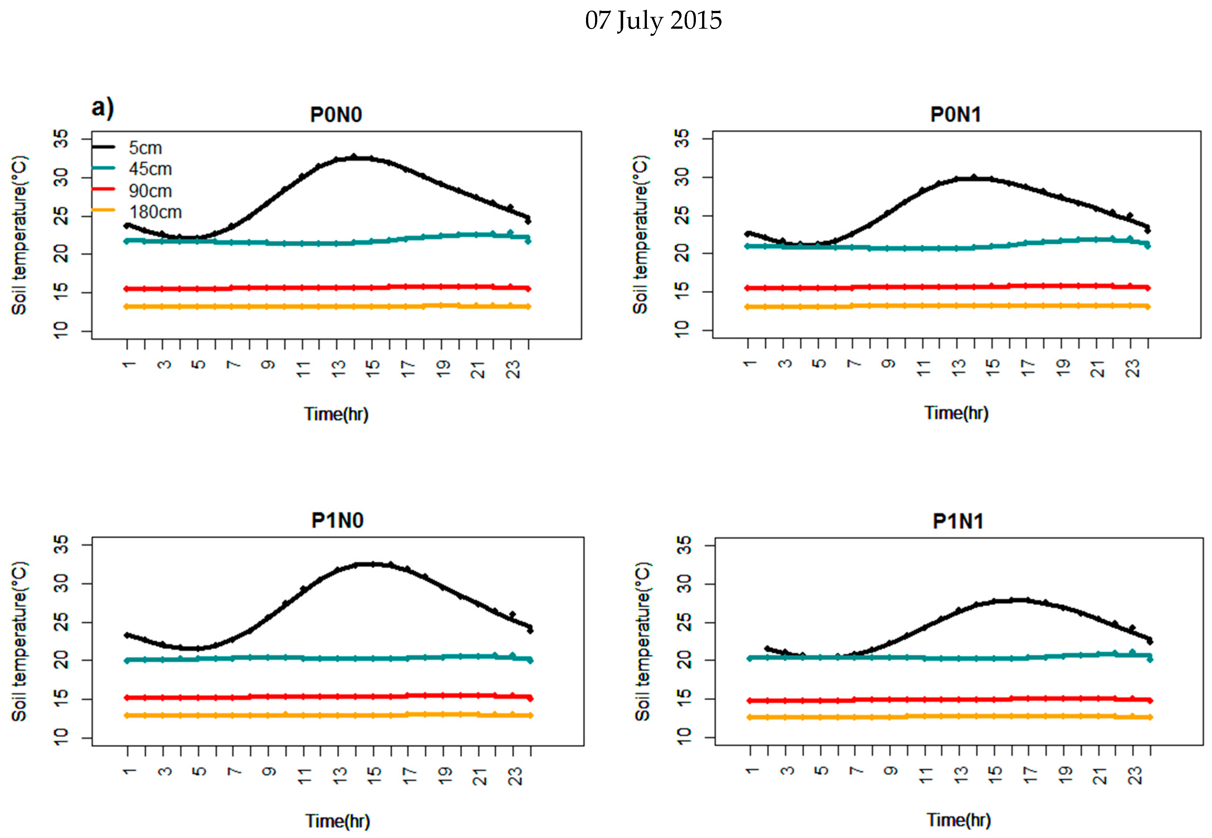
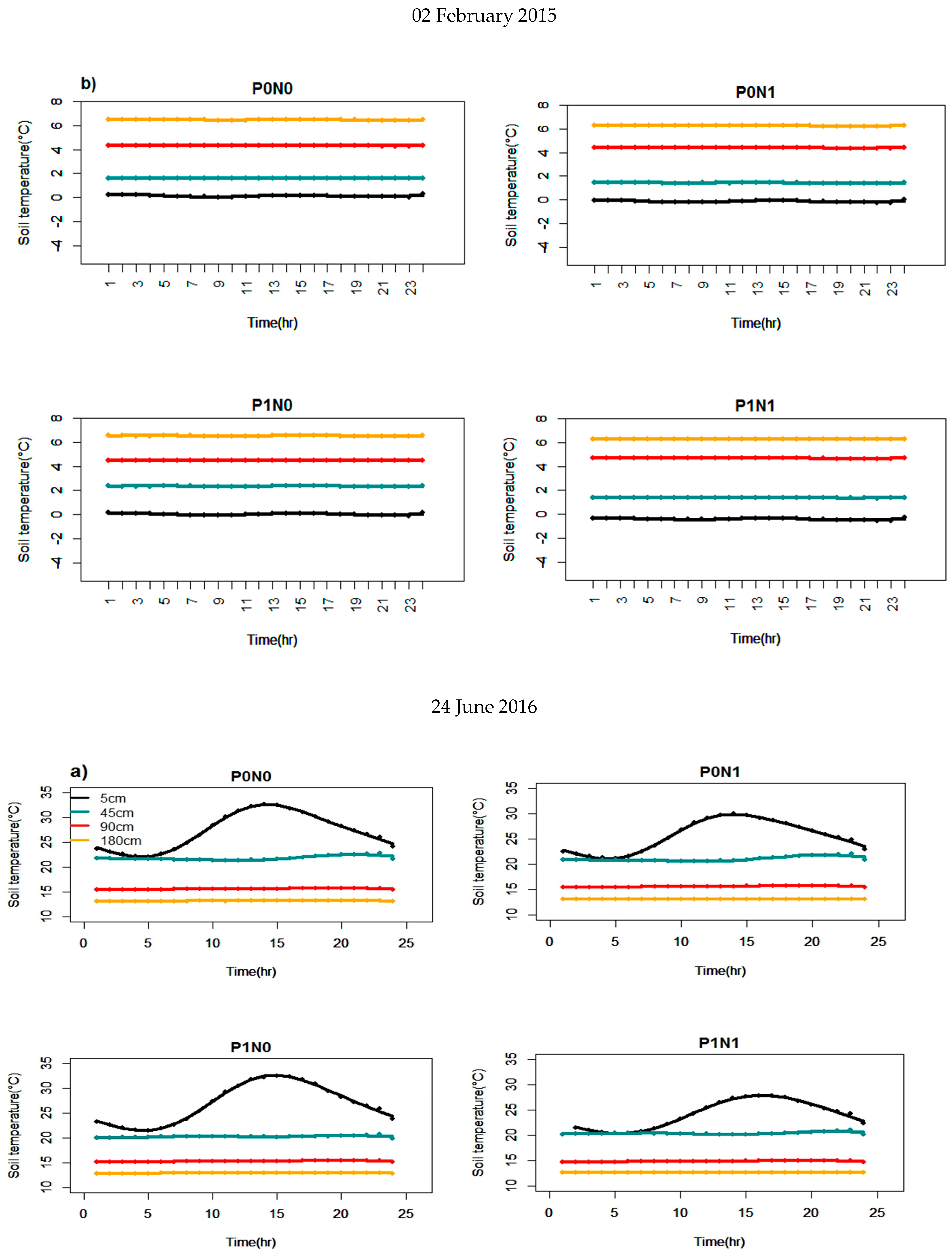
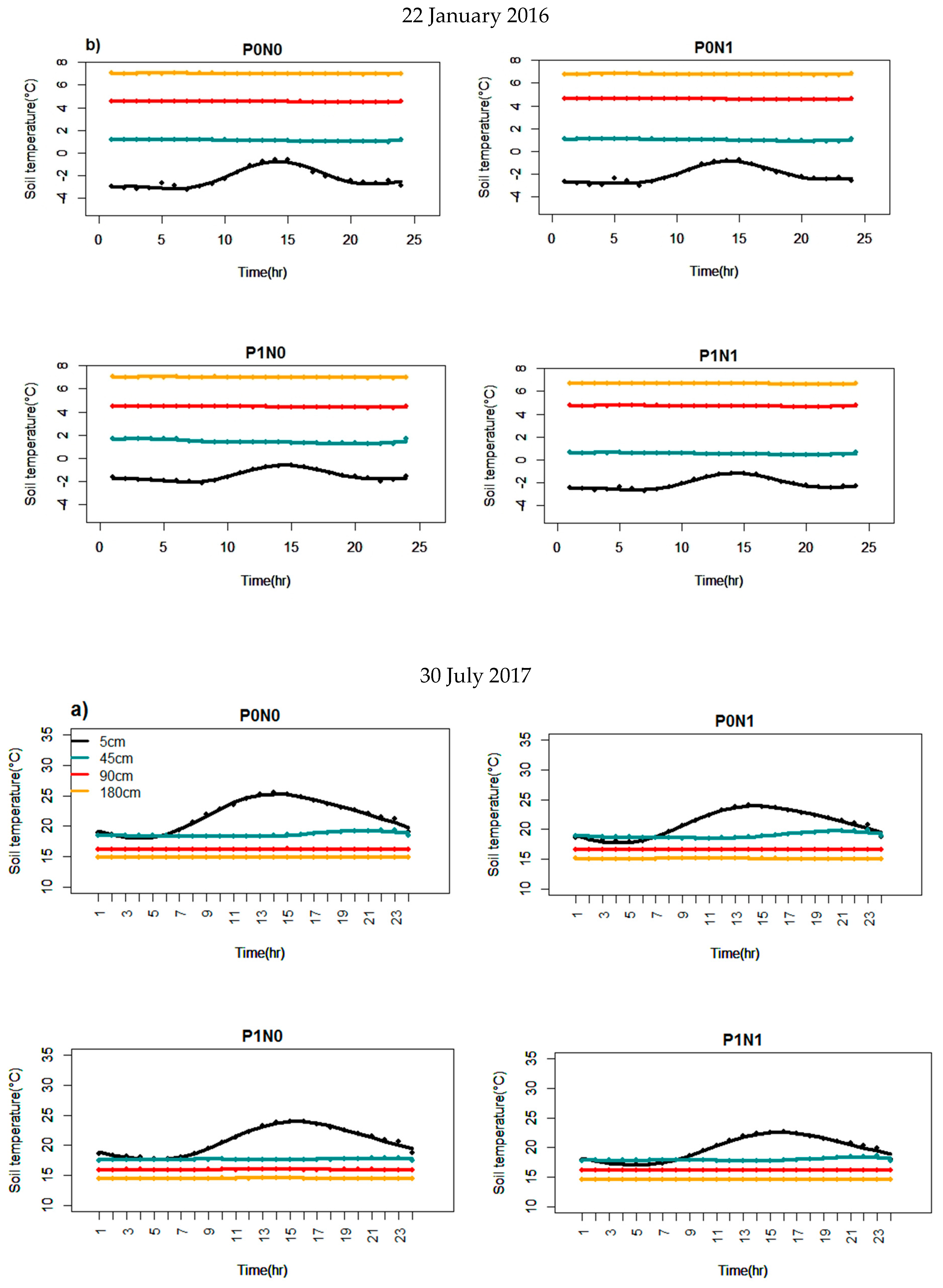
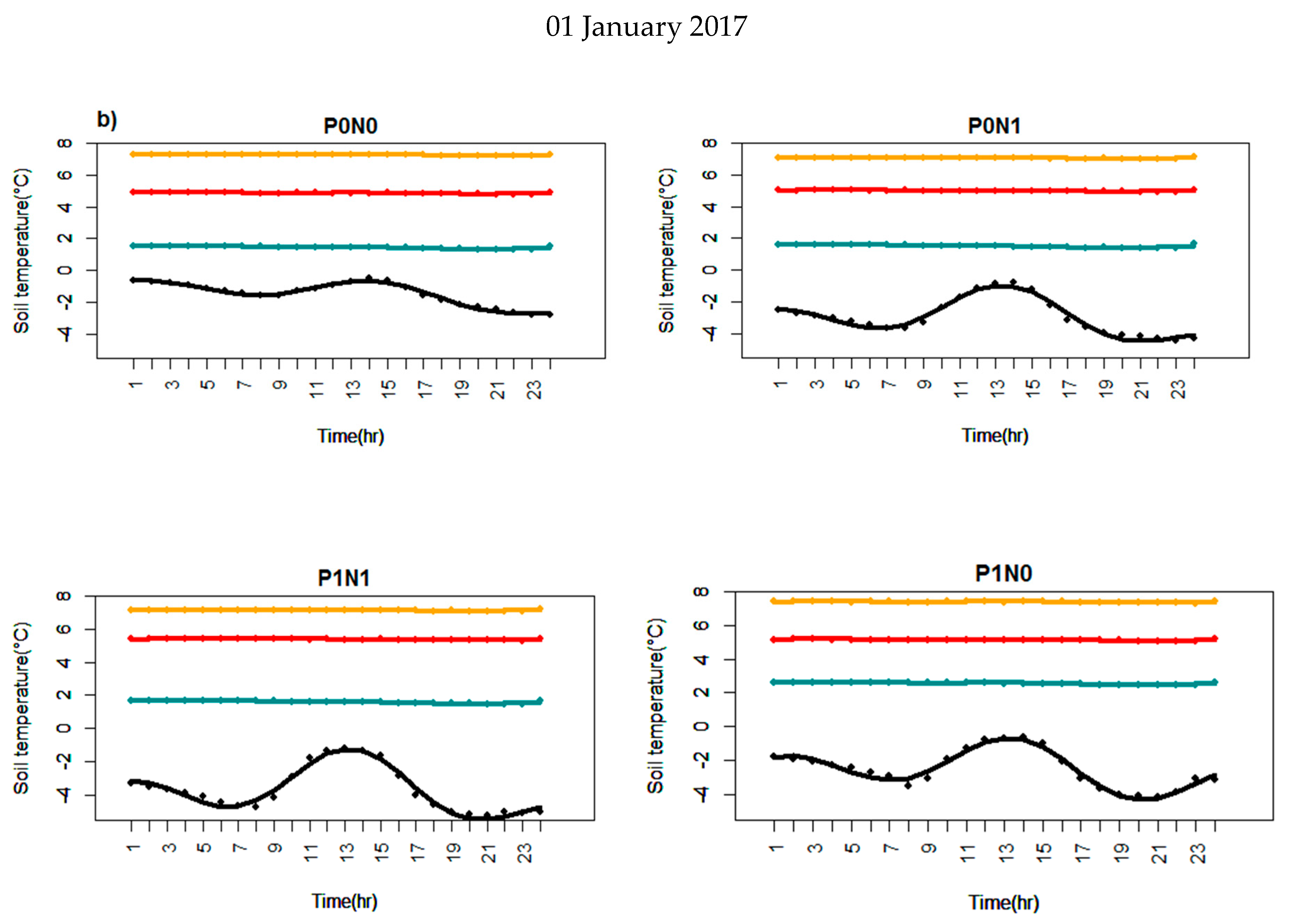
3.2. Diurnal Soil Thermal Behavior in the Soil Layers

To evaluate the most remarkable differences in T_s variations with depth, a continuous-time span from 0:00 to 24:00 with a sinusoidal wave function, was considered for two critical days according to T_air (hottest day of summer months and coldest day of winter months) over the studied period. In 2014, the coldest day was January 26, the warmest day was July 20; in 2015, February 2 and July 7 was the coldest and warmest day, respectively. The coldest day of the year 2016 was January 22, whereas the hottest day for the same year was June 24. The coldest and warmest day in 2017 was January 1 and July 30, respectively. By plotting the hourly measured temperatures at various depths (Figure 2), it is seen that the sinusoidal wave function representation of T_s agreed well with the measured values. The results showed that on the warmest day, the T_s increases from the upper layers downward, while on the coldest day the order is exactly reversed. (Figure 2). Overall, our results show that on the warmest day over the studies years, the temperature of the soil surface starts becoming hot at about 07:00 h and is heated to a higher temperature at about 14:00 h. Due to the high thermal inertia of the soil, the temperature fluctuations at the soil surface are diminished as soil depth increases, so temperature variations were found to be more stable in the greater depths as expected. The heat penetration of the daily cycle is prominent to a depth of about 45 cm and the daily variation below the depth of 45 cm is nearly negligible. This depth depends greatly on the thermal conductivity of the topsoil which is probably relatively low. As Figure 2 shows, changes in amplitude of the soil diurnal temperature wave decreased with increasing soil depth. Since the obtained higher maximum, average T_s, and amplitude of the thermal waves at the shallow depth may result from the incident of radiant energy before further propagation to deeper soil layers and reflection, depending on surface condition. It can be explained that with increasing distance from the exchange surface, heat is stored in each succeeding layer, hence less heat is passed on to the next layer [2,20]. As it can be seen from Figure 2, during the cold day lower fluctuations were found in the 5 cm soil depth over almost all studied years than on the warmest day. T_s fluctuations over the warmest day can hardly be noticed to greater depths than 45 cm (Figure 2), while in the annual course can reach up to 180 cm (Figure 1). Therefore, it shows that temperature fluctuations vary according to temporal courses. These results are in agreement with the findings of [2], who reported that over the day, T_s fluctuations can be reached up to 20–30 cm of soil depth, while seasonal and annual courses can reach up to 2 m and 10 m, respectively. Furthermore, as underlined by [21], diurnal variation of T_s is up to 0.4 m, while annual fluctuation reaches up to a depth of 4 m.

We also evaluated the delay in reaching the maximum and minimum temperatures which occurred in different treatments on the warmest day at the 5 cm soil depth (Figure 3), since on warm days the differences between minimum and maximum daily temperatures among treatments were strongly pronounced. From Figure 3, it can be seen that there was a time shift in the timing of maximum and minimum T_s among treatments. Maximum and minimum T_s did not correspond to 12.00 noon and 00.00 h, respectively. Maximum temperatures on summer day occurred at 14:00 h in P0N0 and P0N1, at 15:00 h in P1N0, and 16:00 h in P1N1. The minimum T_s occurred at about 05:00 h on the summer day in all plots. Thermal waves of the conventional treatments (P1N1) showed lower maximum T_s in all studied years than other treatments, while reduced treatments (P0N0) had high maximum T_s over the studied period (Figure 3). From Figure 3, the amplitude of thermal waves in plots with conventional fertilizer (P0N1, P1N1) is lower than in other plots. Cooler T_s in plots with conventional N fertilizer rate can be explained by the increasing effects of N fertilizer on crop yields and an increase in vegetation cover which result in increasing the absorption of solar energy by the leaves. As crops were at late growth stages in the summer day, the soil surface was covered entirely with plant canopy, thereby shading soil from solar radiation and incidence energy.

3.3. Relationship between Air and Soil Temperature

T_s variations are intimately related to changes in the atmospheric temperature, global solar radiation, and the depth of soil. T_air correlates well with T_s because both are determined by the energy balance at the ground surface. Correlations between T_s and T_air in different depths (5, 45, 90, and 180 cm) of soil under different agricultural managements are demonstrated in

Table 7. Relationship between annual mean air and soil temperatures at different soil depths.

Treatments	Depth (cm)	Equations	p	R2
P0N0	5	Ts = 0.73 + 0.99Tair	***	0.95
	45	Ts = 2.6 + 0.8Tair	***	0.89
	90	Ts = 5 + 0.56Tair	***	0.88
	180	Ts = 6.7 + 0.41Tair	***	0.87
P0N1	5	Ts = 0.86 + 0.93Tair	***	0.93
	45	Ts = 2.3 + 0.8Tair	***	0.91
	90	Ts = 5.1 + 0.56Tair	***	0.88
	180	Ts = 6.5 + 0.42Tair	***	0.88
P1N0	5	Ts = 0.81 + 0.98Tair	***	0.94
	45	Ts = 3.2 + 0.94Tair	***	0.89
	90	Ts = 5.1 + 0.55Tair	***	0.88
	180	Ts = 6.7 + 0.4Tair	***	0.88
P1N1	5	Ts = 0.88 + 0.91Tair	***	0.92
	45	Ts = 2.8 + 0.76Tair	***	0.89
	90	Ts = 5.4 + 0.54Tair	***	0.88
	180	Ts = 6.5 + 0.4Tair	***	0.88

T_air: annual mean air temperature (°C); T_s: annual mean soil temperature (°C). R²: determinant coefficient; P: significance level, *** significant difference at the 0.001 probability level.

. Regression analysis revealed that daily T_s could be predicted efficiently with the help of corresponding mean T_air by considering the time lag that exists between T_air and T_s at different depths. A general understanding of how T_air relates to T_s is that the amplitudes of T_s are dampened and its phase is shifted against T_air due to heat transport processes. R² values showed that the prediction of T_s using mean T_air could explain more than 90% variability of T_s for topsoil. While the accuracy of predicting T_s in the subsoil is slightly less than in the topsoil. In this study, linear regressions are considered regional equations. As underlined by [17], the above method can be used in such cases when the database of measurement is not complete. The application of the regression equation can supplement the use of the time-consuming T_s measuring method.

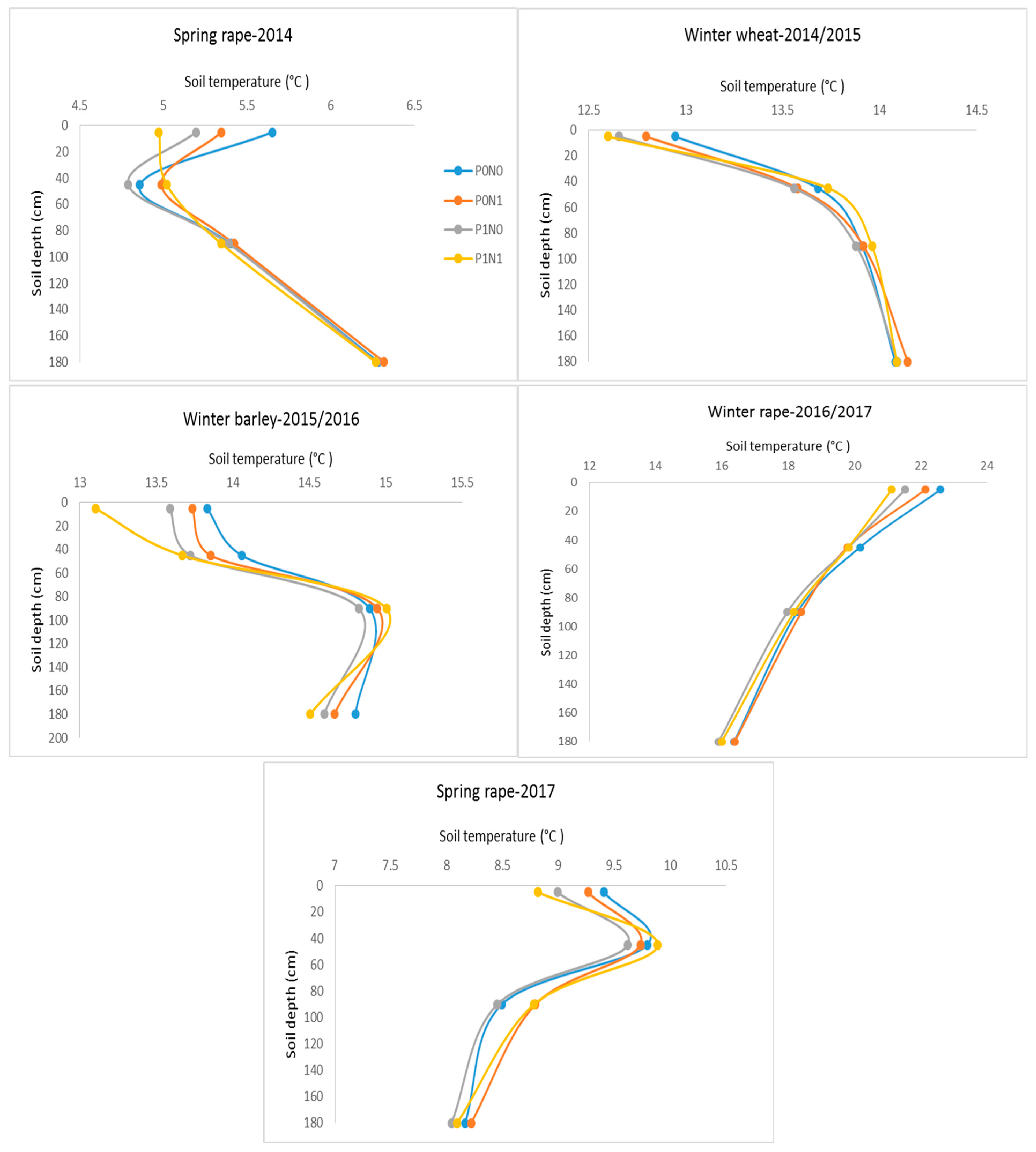
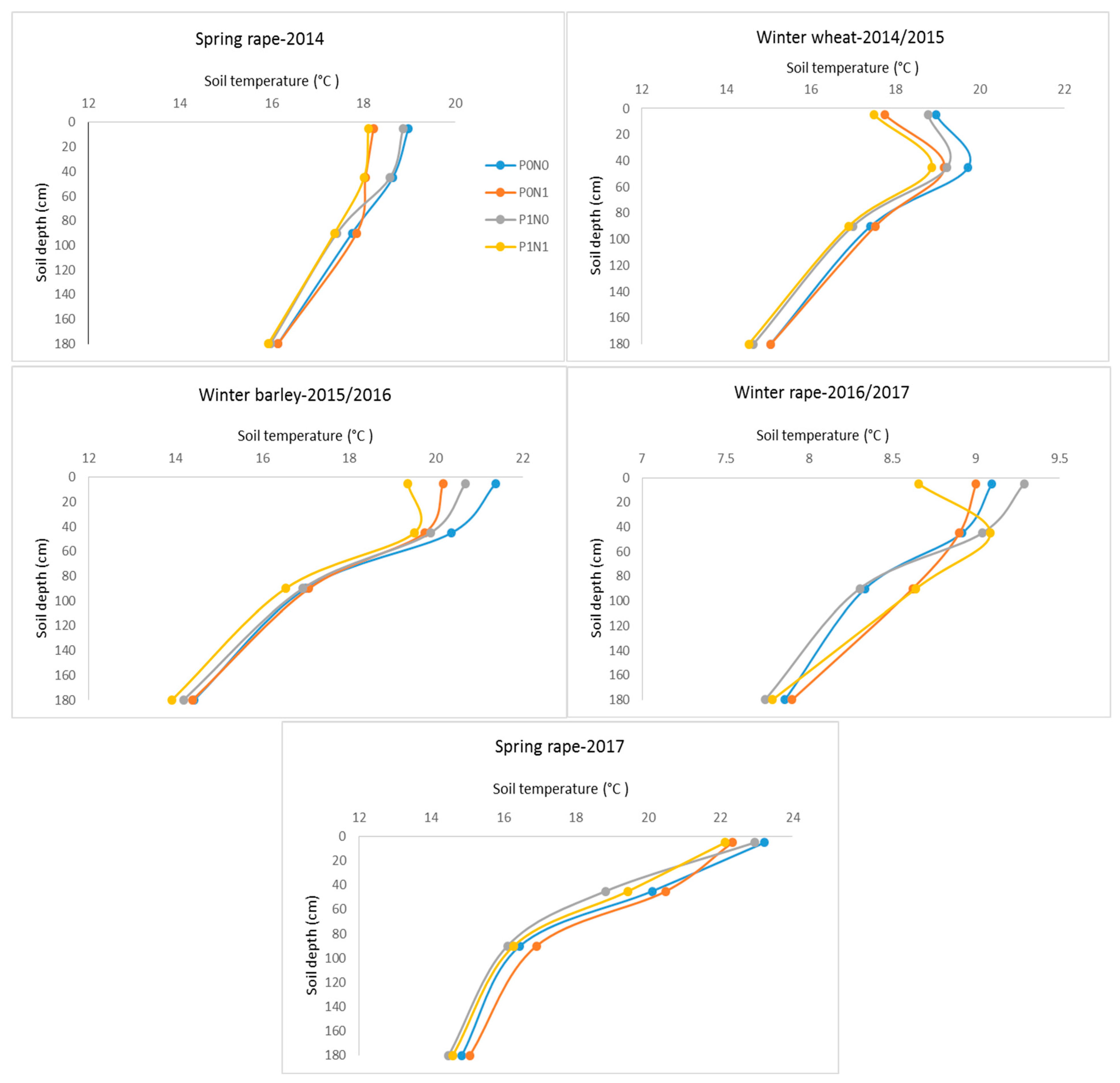
3.4. Temporal Soil Temperature Changes at Sowing and a Day before Harvest Time in Different Soil Layers

The effect of the management practices on the temperature fluctuations is related to the period during the year, due to the impacts of fertilizer on the crop canopy, and the effects of soil tillage on surface roughness and porosity. T_s is important for seed germination and is a reason why we selected the sowing date for determining the effect of management on T_s variations. T_s and soil moisture conditions in the seedbed zone can improve or delay seed germination and plant emergence.

Effects of treatments on T_s at sowing date at different depths are shown in Figure 4. Our results showed that at the sowing date, a higher T_s was observed under P0N0 and P0N1 than in P1N0 and P1N1 plots, which likely contributed primarily to higher residue coverage under T_R plots than T_C plots (Table 5). Surface residue cover can affect soil temperature by insulating the soil surface and slowing soil drying. The effect of plant residues on reducing soil cooling during the period with low temperatures could be responsible for higher T_s under T_R. In our experiment, straw stayed on the field and was evenly distributed on the soil surface after harvest to protect the soil and improve soil organic carbon. Since crop rotations were very close and there was little time for straw rotting between harvest and new sowing, residues should be mixed into the soil. Under P1N0 and P1N1 plots, residues were accommodated in deeper soil layers than in P0N0 and P0N1 plots, and the lack of an insulating layer of crop residue could be a reason why our results did show higher T_s in P0N0 and P0N1 plots at the sowing date. Since in this study, spring rape was planted in early spring, winter wheat, winter barley, and winter rape were planted in early autumn, the presence of plant residues on the soil surface insulates the soil from colder T_air and decreases heat loss. It has been reported that straw can protect the soil from extreme thermal conditions that could make soil nutrients immobile and soil micro-organisms to be dormant [15]. It is speculated from this result to some extent that higher T_s in T_R plots can be profitable in the sowing period, improving crop establishment. As reported by [22], suitable T_s can significantly accelerate seed germination during the early stage of crop growth.

On the other hand, soil bulk density in conventional tillage systems could be lower than reduced tillage, resulting in more pore space, which is filled with air and water. As air is a good insulator with low thermal conductivity and the flow of heat is lower in dry soil where the pores are filled with air, it can be contributed to low temperature in T_C. Furthermore, T_R soils with straw residues in topsoil can retain more water than T_C soils; consequently, soil heat capacity would be increased and lead to absorbing a lot of heat for changing temperature [23]. As underlined by [24], the temperature-increasing effect of straw coverage was mainly derived from perseveration of soil moisture, increase in soil thermal capacity, and blockage of long-wavelength radiation on the soil surface thus leading to an alleviated reduction in T_s underneath the coverage. Conversely, in higher soil bulk density, the contact between particles is increased, and; consequently, the soil thermal conductivity increases [25], leading to higher T_s in T_R. Therefore, it can be concluded that differences in T_s in both tillage systems could be due to differences in mulch remaining after soil management. These results are consistent with those reported by [20,26].

The late plant growth and development stage (one day before harvest) was also selected as one of the important crop stages in the growing season to assess the effect of applied treatments on T_s at various depths (Figure 5). The four–year experiments indicated that at the late plant growth stage, applying reduced N fertilizers in a reduced tillage plot (P0N0) increased the T_s compared to conventional N fertilizer and conventional tillage plot (P1N1) at 5 cm soil depth with 0.9 °C under spring rape-2014, 1.5 °C under winter wheat-2014/2015, 2 °C under winter barley-2015/2016, 0.5 °C under Winter rape-2016/2017, and 1.1 °C under Spring rape-2017 (Figure 5). In the late plant growth stages, the canopy covers the ground and prevents solar radiation, resulting in reduction of airflow, evaporation intensity, and transfer of water and heat between soil and atmosphere giving rise to soil surface temperature reduction. Thus, we can speculate from this result that in this plant growth stage, the effect of plant coverage on T_s variations is mainly driven by the N fertilizer application and are less related to the tillage systems. Table 5 provides the crop yields during the studied years. From Table 5, plots with receiving a standard rate of N fertilization had higher grain and straw yields with higher plant coverage and shading effect than plots with reduced N fertilization. Throughout the monitoring period, the effect of treatments on T_s was consistent and not varied by crop rotation at the sowing and the last day before harvest, and these effects were gradually reduced with the soil layer deepening (Figure 4 and Figure 5).

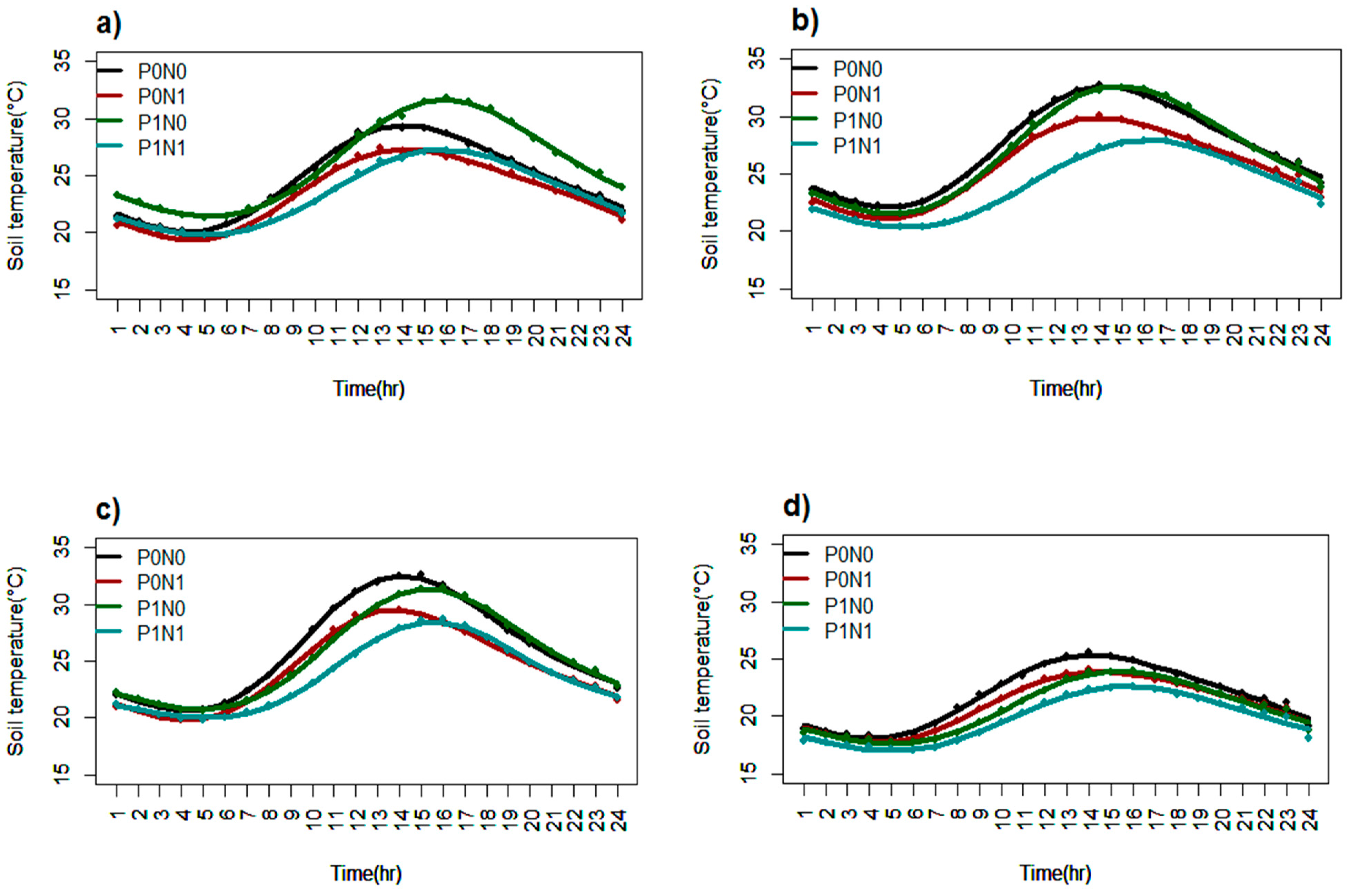
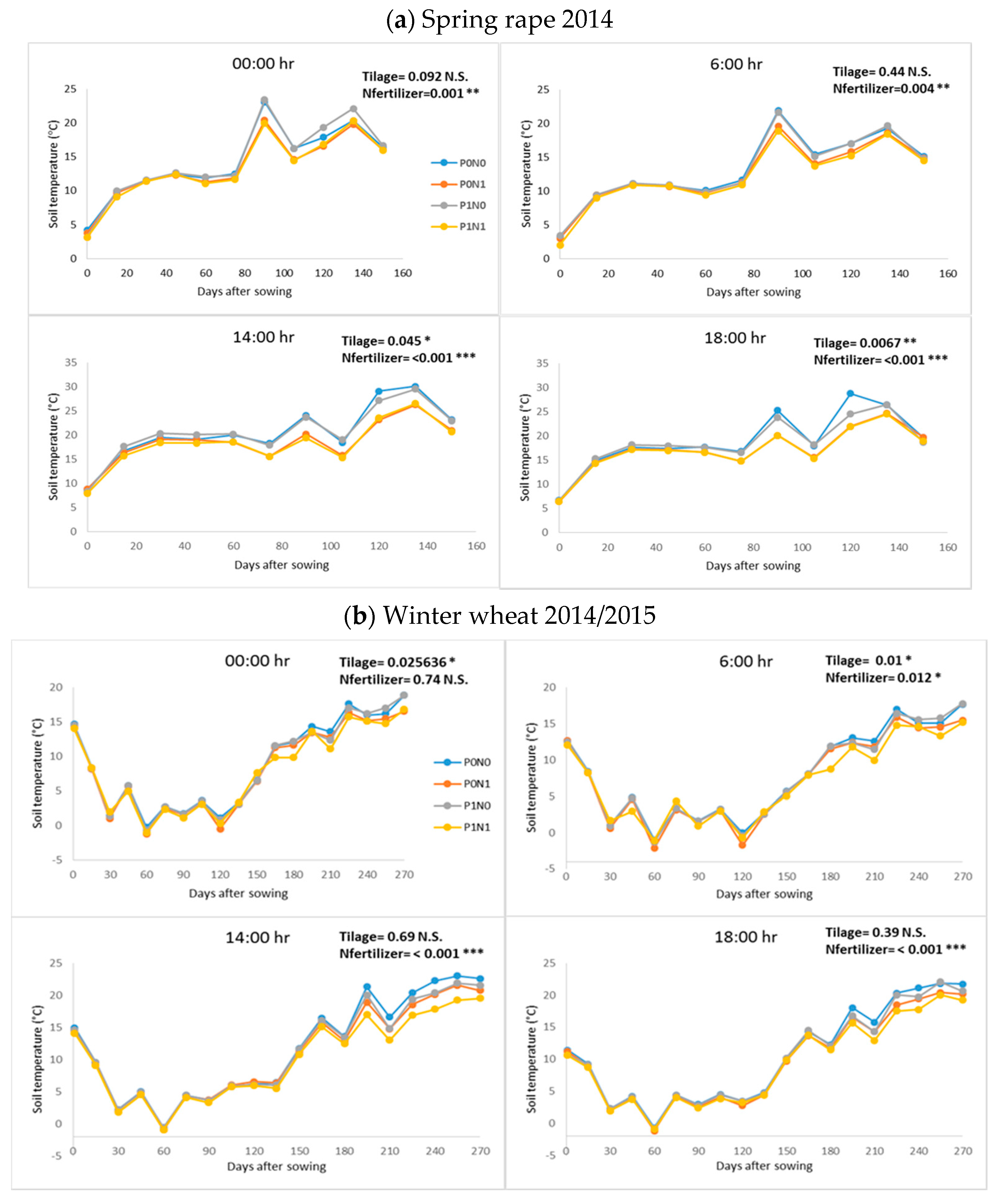
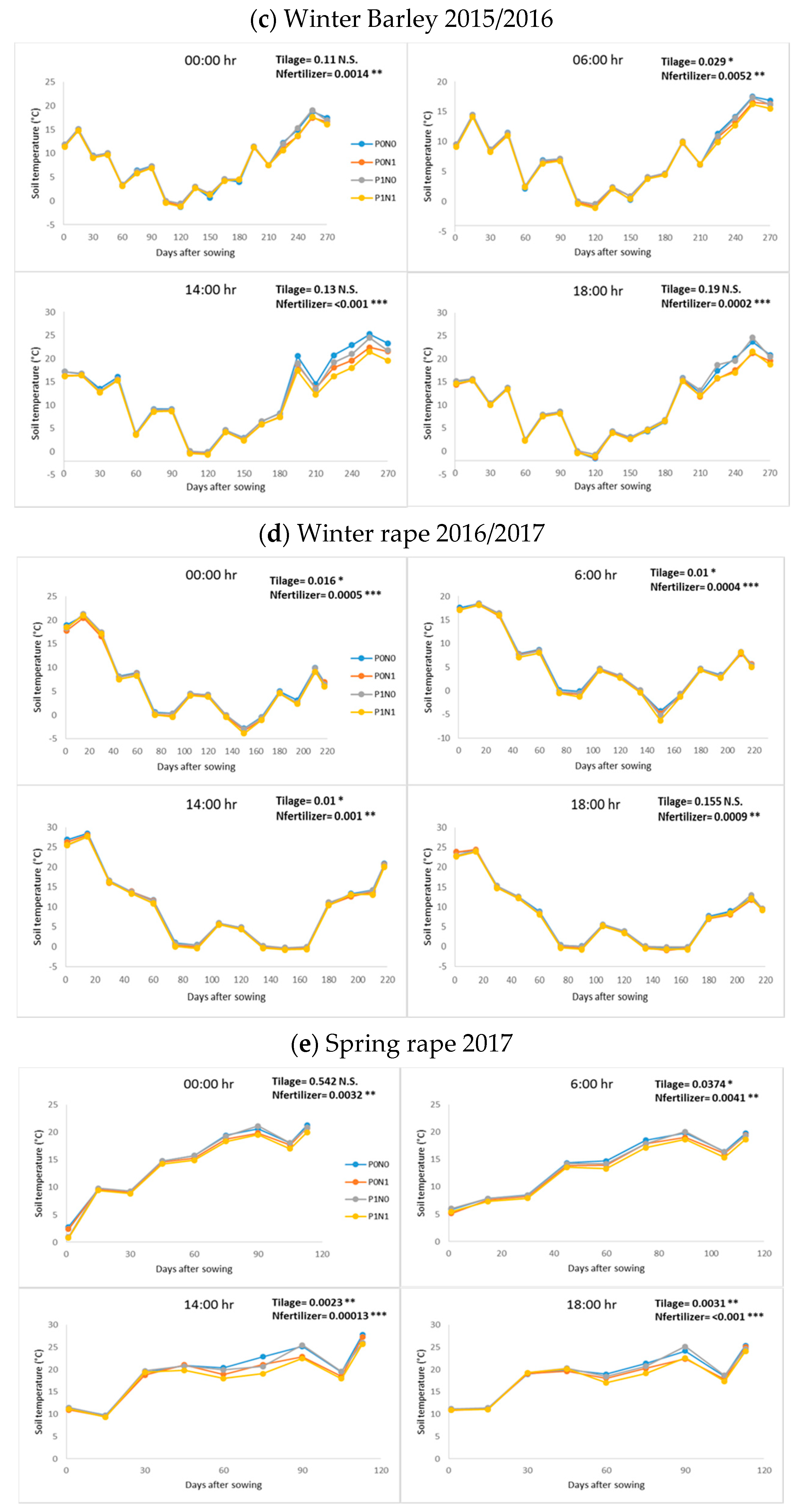
3.5. Topsoil Temperature Variation at Different Day Times during Days after Sowing

The fluctuations of T_s in 5 cm under various managements during days after sowing (DAS) are shown in Figure 6. Irrespective of the management systems, T_s in all plots are gradually decreased after 00:00 h until 06:00 h, increased after 06:00 h, and reached a peak at 14:00 h, followed by a decrease after 18:00 h over the years of the experiment (Figure 6), as also found in a previous study [27].

At 00:00 h, differences in the T_s in 5 cm among treatments were less. However, the T_s differences were slightly higher after 06:00 h.

At 06:00 h, during spring rape growth season, the difference in T_s among various treatments increased from 60 DAS. The most incredible difference in T_s among treatments under spring rape growth season was 2.98 °C and 1.44 °C at 90 DAS in 2014 and 2017, respectively; thereafter, the magnitude of difference decreased with the advance of the cropping period (Figure 6a,e). During growing seasons of winter wheat and winter rape, the T_s differences during the early hours of the day (06:00 h) among treatments increased from 30, and 135 DAS, respectively. The differences among treatments were highest at 180 DAS under winter wheat (3.19 °C) and 150 DAS under winter rape (1.1 °C) (Figure 6b,c). While the increase of T_s differences among treatments under winter barley was observed from 225 DAS (Figure 6c).

The T_s was highest at 14:00 h, and the difference was also the largest. The differences among treatments under crop rotation systems were highly pronounced in the middle hours of the day when T_air reached its maximum. The differences in T_s are more evident on the earlier days after sowing at 14:00 h compared to other hours of the day. The highest difference in T_s among treatments was 5.49 °C and 3.81 °C at the mid-late of DAS in 2014 and 2017, respectively (Figure 6a,e). Whereas the greatest T_s differences of winter wheat, winter barley, and winter rape, at 14:00 h, were 4.34 °C, 3.2 °C, and 1.14 °C, respectively (Figure 6b–d). In the evening, at 18:00 h, the T_s was moderate, and the differences among treatments are reduced. This trend followed a similar pattern during the studied period.

The interactive effects of the tillage with N fertilizer practices on the T_s may depend on the crop growing period during the experimental years. Irrespective of the N fertilizer rate, at the early growth stage, the mean T_s in 5 cm was highest in the reduced tillage plots (P0N0, P0N1) and lowest in the conventional tillage plots (P1N0, P1N1) during 2014–2017; however, these differences were lasted up to 30 DAS. The changes in T_s under treatments at the sowing date may be in part due to the influence of tillage on surface residue cover. Reduced tillage decreases the intensity and frequency of soil disturbance, compared to conventional tillage, i.e., the crop residues on the soil surface was reduced by greater plowing depth.

Since crops were sown almost in the cool months, more crop residue in T_R leads to greater conservation of heat under T_R. Furthermore, decaying crop residues with time reduced the impact of straw on the T_s. Although T_R contributes to higher amounts of surface crop residues in cropping systems, the effect of tillage on T_s diminishes with an increase in percent ground cover and shading of soil. Part of the N fertilizer was applied at the mid-growth stage, which resulted in the greatest effect of N fertilizer on higher crop yield in plots receiving conventional N fertilizer (P0N1, P1N1) and having low T_s at the final growth stage (Table 5, Figure 6). These findings agree with those obtained by [27,28].

4. Conclusions

This study provides insights into changes in T_s induced by tillage practices and fertilization in croplands. The measured T_s at different soil depths were periodic because of variations in daily and seasonal solar radiation, and showed similar fluctuations from year to year during the studied period. Shallower depths were more affected by the heat from the surface, related to incident solar radiation, and then dictates the land surface temperature dynamics. The soil surface is more sensitive than deeper soil to temperature changes, thus the amplitudes of the measured soil temperatures decreased as the soil depths increased.

Lower temperature in cold months is one of the main limitations on planting, germination, and emergence, and the early growth of crops as well. The effects of tillage systems on soil temperature can help explain some of the differences in plant growth and development in different tillage systems. Findings showed that reduced tillage practice improved soil thermal status in the cold months and created an ideal T_s condition in seedbed zones for plant emergence and plant development. The effect of tillage practices on T_s became attenuated at the last vegetation stages; however, fertilization application showed a greater impact on T_s variation. Given the applied management practices in croplands, short-term studies might not provide enough information, so long-term experiments are an indispensable prerequisite for coming to a thorough a complete understanding of management-induced changes in T_s. Since long-term management practices gradually affect soil physical and chemical properties and consequently soil thermal properties.

Understanding the response of T_s dynamic to management could be advantageous for many different areas of environmental science and climatology. T_s as an effective factor might be used in future solutions to climate changes, optimizing management practices, predicting carbon, nitrogen, and water dynamics, and other related processes as well. Furthermore, since soil water content, soil type, heat flow density, and heat capacity are influential factors for soil processes, therefore, these factors should be taken into account in future studies to consider their interaction effects on T_s.

References

1. Huang, R.; Huang, J.-X.; Zhang, C.; Ma, H.-Y.; Zhuo, W.; Chen, Y.-Y.; Zhu, D.-H.; Wu, Q.; Mansaray, L.R. Soil temperature estimation at different depths, using remotely-sensed data. J. Integr. Agric. 2020, 19, 277–290. [Google Scholar] [CrossRef]
2. Muñoz-Romero, V.; Lopez-Bellido, L.; Lopez-Bellido, R.J. Effect of tillage system on soil temperature in a rainfed Mediterranean Vertisol. Int. Agrophysics 2015, 29, 467–473. [Google Scholar] [CrossRef] [Green Version]
3. Moroizumi, T.; Horino, H. The effects of tillage on soil temperature and soil water. Soil Sci. 2002, 167, 548–559. [Google Scholar] [CrossRef]
4. Yang, Y.; Ding, J.; Zhang, Y.; Wu, J.; Zhang, J.; Pan, X.; Gao, C.; Wang, Y.; He, F. Effects of tillage and mulching measures on soil moisture and temperature, photosynthetic characteristics and yield of winter wheat. Agric. Water Manag. 2018, 201, 299–308. [Google Scholar] [CrossRef]
5. Li, Y.; Li, Z.; Cui, S.; Jagadamma, S.; Zhang, Q. Residue retention and minimum tillage improve physical environment of the soil in croplands: A global meta-analysis. Soil Tillage Res. 2019, 194, 104292. [Google Scholar] [CrossRef]
6. Liu, S.; Li, J.; Zhang, X. Simulations of Soil Water and Heat Processes for No Tillage and Conventional Tillage Systems in Mollisols of China. Land 2022, 11, 417. [Google Scholar] [CrossRef]
7. Singh, B. Are Nitrogen Fertilizers Deleterious to Soil Health? Agronomy 2018, 8, 48. [Google Scholar] [CrossRef] [Green Version]
8. Zhong, Y.; Wang, X.; Yang, J.; Zhao, X.; Ye, X. Exploring a suitable nitrogen fertilizer rate to reduce greenhouse gas emissions and ensure rice yields in paddy fields. Sci. Total Environ. 2016, 565, 420–426. [Google Scholar] [CrossRef]
9. Lian, Y.; Meng, X.; Yang, Z.; Wang, T.; Ali, S.; Yang, B.; Zhang, P.; Han, Q.; Jia, Z.; Ren, X. Strategies for reducing the fertilizer application rate in the ridge and furrow rainfall harvesting system in semiarid regions. Sci. Rep. Cetacean Res. 2017, 7, 2644. [Google Scholar] [CrossRef] [Green Version]
10. Altermann, M.; Rinklebe, J.; Merbach, I.; Körschens, M.; Langer, U.; Hofmann, B. Chernozem—Soil of the Year 2005. J. Plant Nutr. Soil Sci. 2005, 168, 725–740. [Google Scholar] [CrossRef]
11. Horton, R.; Wierenga, P.J.; Nielsen, D.R. Evaluation of Methods for Determining the Apparent Thermal Diffusivity of Soil Near the Surface. Soil Sci. Soc. Am. J. 1983, 47, 25–32. [Google Scholar] [CrossRef]
12. R Core Team. A Language and Environment for Statistical Computing; R Core Team: Vienna, Austria, 2013. [Google Scholar]
13. Zhan, M.-J.; Xia, L.; Zhan, L.; Wang, Y. Recognition of Changes in Air and Soil Temperatures at a Station Typical of China’s Subtropical Monsoon Region (1961–2018). Adv. Meteorol. 2019, 2019, 6927045. [Google Scholar] [CrossRef] [Green Version]
14. Park, K.; Kim, Y.; Lee, K.; Kim, D. Development of a Shallow-Depth Soil Temperature Estimation Model Based on Air Temperatures and Soil Water Contents in a Permafrost Area. Appl. Sci. 2020, 10, 1058. [Google Scholar] [CrossRef] [Green Version]
15. Hu, Q.; Feng, S. A Daily Soil Temperature Dataset and Soil Temperature Climatology of the Contiguous United States. J. Appl. Meteorol. 2003, 42, 1139–1156. [Google Scholar] [CrossRef]
16. Fang, X.; Luo, S.; Lyu, S. Observed soil temperature trends associated with climate change in the Tibetan Plateau, 1960–2014. Theor. Appl. Climatol. 2019, 135, 169–181. [Google Scholar] [CrossRef] [Green Version]
17. Pokladníková, H.; RožnovSký, J.; STředa, T. Evaluation of soil temperatures at agroclimatological station Pohořelice. Soil Water Res. 2008, 3, 223–230. [Google Scholar] [CrossRef] [Green Version]
18. Florides, G.A.; Kalogirou, S.A. Annual ground temperature measurements at various depths. In Proceedings of the CLIMA 2005, Lausanne, Switzerland, 9–12 October 2005. [Google Scholar]
19. Dec, D.; Dörner, J.; Horn, R. Effect of soil management on their thermal properties. J. Soil Sci. Plant Nutr. 2009, 9, 26–39. [Google Scholar] [CrossRef]
20. Awe, G.O.; Reichert, J.M.; Wendroth, O.O. Temporal variability and covariance structures of soil temperature in a sugarcane field under different management practices in southern Brazil. Soil Tillage Res. 2015, 150, 93–106. [Google Scholar] [CrossRef]
21. Singh, R.K.; Sharma, R.V. Numerical analysis for ground temperature variation. Geotherm. Energy 2017, 5, 22. [Google Scholar] [CrossRef] [Green Version]
22. Zhao, H.; Xiong, Y.-C.; Li, F.-M.; Wang, R.-Y.; Qiang, S.-C.; Yao, T.-F.; Mo, F. Plastic film mulch for half growing-season maximized WUE and yield of potato via moisture-temperature improvement in a semi-arid agroecosystem. Agric. Water Manag. 2012, 104, 68–78. [Google Scholar] [CrossRef]
23. Zapata, D.; Rajan, N.; Mowrer, J.; Casey, K.; Schnell, R.; Hons, F. Long-term tillage effect on with-in season variations in soil conditions and respiration from dryland winter wheat and soybean cropping systems. Sci. Rep. 2021, 11, 2344. [Google Scholar] [CrossRef] [PubMed]
24. Liang, H.; Hu, K.; Qin, W.; Zuo, Q.; Zhang, Y. Modelling the effect of mulching on soil heat transfer, water movement and crop growth for ground cover rice production system. Field Crops Res. 2017, 201, 97–107. [Google Scholar] [CrossRef]
25. Abu-Hamdeh, N.H.; Reeder, R.C. Soil Thermal Conductivity Effects of Density, Moisture, Salt Concentration, and Organic Matter. Soil Sci. Soc. Am. J. 2000, 64, 1285–1290. [Google Scholar] [CrossRef]
26. Sharratt, B.S. Corn stubble height and residue placement in the northern US Corn Belt: Part I. Soil physical environment during winter. Soil Tillage Res. 2002, 64, 243–252. [Google Scholar] [CrossRef]
27. Hou, X.; Li, R. Interactive effects of autumn tillage with mulching on soil temperature, productivity and water use efficiency of rainfed potato in loess plateau of China. Agric. Water Manag. 2019, 224, 105747. [Google Scholar] [CrossRef]
28. Wang, Y.; Chen, S.; Sun, H.; Zhang, X. Effects of different cultivation practices on soil temperature and wheat spike differentiation. Cereal Res. Commun. 2009, 37, 575–584. [Google Scholar] [CrossRef]
Figure 1. Fitted annual soil thermal waves of different treatments at various soil depths over the studied years. (a) P0N0 (b) P0N1 (c) P1N0 and (d) P1N1.
Agronomy 12 01199 g001aAgronomy 12 01199 g001b
Figure 2. Soil temperature variation for the (a) hottest day and (b) coldest day under different managements over the studied years.
Agronomy 12 01199 g002aAgronomy 12 01199 g002bAgronomy 12 01199 g002cAgronomy 12 01199 g002dAgronomy 12 01199 g002e
Figure 3. Variation of the soil temperature at 5 cm soil depth for the hottest day under various management over the studied years: (a) 2014 (b) 2015 (c) 2016 (d) 2017.
Agronomy 12 01199 g003
Figure 4. Soil temperature (°C) at different soil depths according to the fertilizer rate and tillage system on sowing day.
Agronomy 12 01199 g004
Figure 5. Soil temperature (°C) at different soil depths according to the fertilizer rate and tillage system at the late plant growth stage.
Agronomy 12 01199 g005
Figure 6. Soil temperature (°C) variation at 5 cm soil layer under tillage and N fertilizer practices at the 0, 6, 14, and 18 h during the days after spring rape sowing (2014). * Significant difference at the 0.05 probability level, ** significant difference at the 0.01 probability level, *** significant difference at the 0.001 probability level, N.S. not significant by least significant different test (LSD 0.05).
Agronomy 12 01199 g006aAgronomy 12 01199 g006b