Predicting Soil Organic Carbon and Total Nitrogen at the Farm Scale Using Quantitative Color Sensor Measurements

Abstract

Sensor technology can be a reliable and inexpensive means of gathering soils data for soil health assessment at the farm scale. This study demonstrates the use of color system readings from the Nix Pro^TM color sensor (Nix Sensor Ltd., Hamilton, ON, Canada) to predict soil organic carbon (SOC) as well as total nitrogen (TN) in variable, glacial till soils at the 147 ha Cornell University Willsboro Research Farm, located in Upstate New York, USA. Regression analysis was conducted using the natural log of SOC (lnSOC) and the natural log of TN (lnTN) as dependent variables, and sample depth and color data were used as predictors for 155 air dried soil samples. Analysis was conducted for combined samples, Alfisols, and Entisols as separate sample sets and separate models were developed using depth and color variables, and color variables only. Depth and L* were significant predictors of lnSOC and lnTN for all sample sets. The color variable b* was not a significant predictor of lnSOC for any soil sample set, but it was for lnTN for all sample sets. The lnSOC prediction model for Alfisols, which included depth, had the highest R² value (0.81, p-value < 0.001). The lnSOC model for Entisols, which contained only color variables, had the lowest R² (0.62, p-value < 0.001). The results suggest that the Nix Pro^TM color sensor is an effective tool for the rapid assessment of SOC and TN content for these soils. With the accuracy and low cost of this sensor technology, it will be possible to greatly increase the spatial and temporal density of SOC and TN estimates, which is critical for soil management.

1. Introduction

Rapid and accurate estimates of soil organic carbon (SOC) and total nitrogen (TN) are important in soil fertility assessment and there is a need for rapid methods to monitor and assess soil health and quality especially at the farm scale [1,2,3,4]. Standard methods of SOC quantification (e.g., chemical oxidation, dry combustion) are not always portable for in field evaluation [5]. Recent research demonstrated a strong relationship between SOC and soil color [6,7,8,9,10]. The use of spectrometers for remote sensing or rapid analysis of soils data allows for data collection at a much higher spatial resolution and at a more rapid rate [11]. However, spectrometers can often be very expensive to purchase and may require special training to use and understand spectral results to develop calibrated prediction models for each sample [7,12].

The Minolta CR-400TM chromameter (Konica Minolta Sensing Americas, Inc., Ramsey, NJ, USA) was recently used to predict soil carbon using ordinary least squares analysis [13]. The chromameter is a handheld device that produces quantitative color results in the color system readings defined by the Commission Internationale de l’Eclairage (CIE) as the CIE L* a* b* color system (L* = lightness to darkness, a* = green to red, b* = blue to yellow) which allow for a more straight forward statistical analysis. Soil darkness (L*) was used as a continuous predictor of soil carbon. Again, the researchers’ results suggest that the visible range can be used to successfully predict soil carbon. However, the Minolta CR-400TM is limited by its power requirements and is relatively expensive which may reduce the applicability of the device as a tool to predict and monitor SOC (http://sensing.konicaminolta.us/).

Devices that measure in the visible range are often less expensive, but color results from the Konica Minolta CR-400 were comparable to an inexpensive color sensor, the Nix Pro™ (https://nixsensor.com) [14]. The sensor is small in size, rechargeable, and contains its own LED light source making it a very mobile method of color determination. Multiple color systems, including CIE L* a* b*, are reported via a mobile application which controls the sensor through Bluetooth™ connections. The sensor is also inexpensive, costing approximately $349 (https://nixsensor.com). Nix Pro™ was tested as a means of SOC prediction using soil color data in Ultisols of South Carolina using regression analysis [15]. It was also used to predict SOC and TN in the Russian Chernozem using soil color and depth [16]. These results suggest that soil color measured in the visible range with the Nix Pro^TM color sensor can be effectively used to predict SOC and TN in two soil orders (Ultisols and Mollisols). Use of a low-cost sensor to estimate SOC and TN could increase the number of measurements in agriculture and environmental sciences [17]. The overall objective of this study was to predict SOC and TN on a farm using depth and quantitative color sensor measurements. The specific objectives were: (i) to develop SOC and TN prediction models for multiple soil types collectively; (ii) to determine if dividing soils into individual soil orders before model development improves prediction accuracy; and (iii) to determine if color variables alone are sufficient predictors of SOC and TN.

2. Materials and Methods

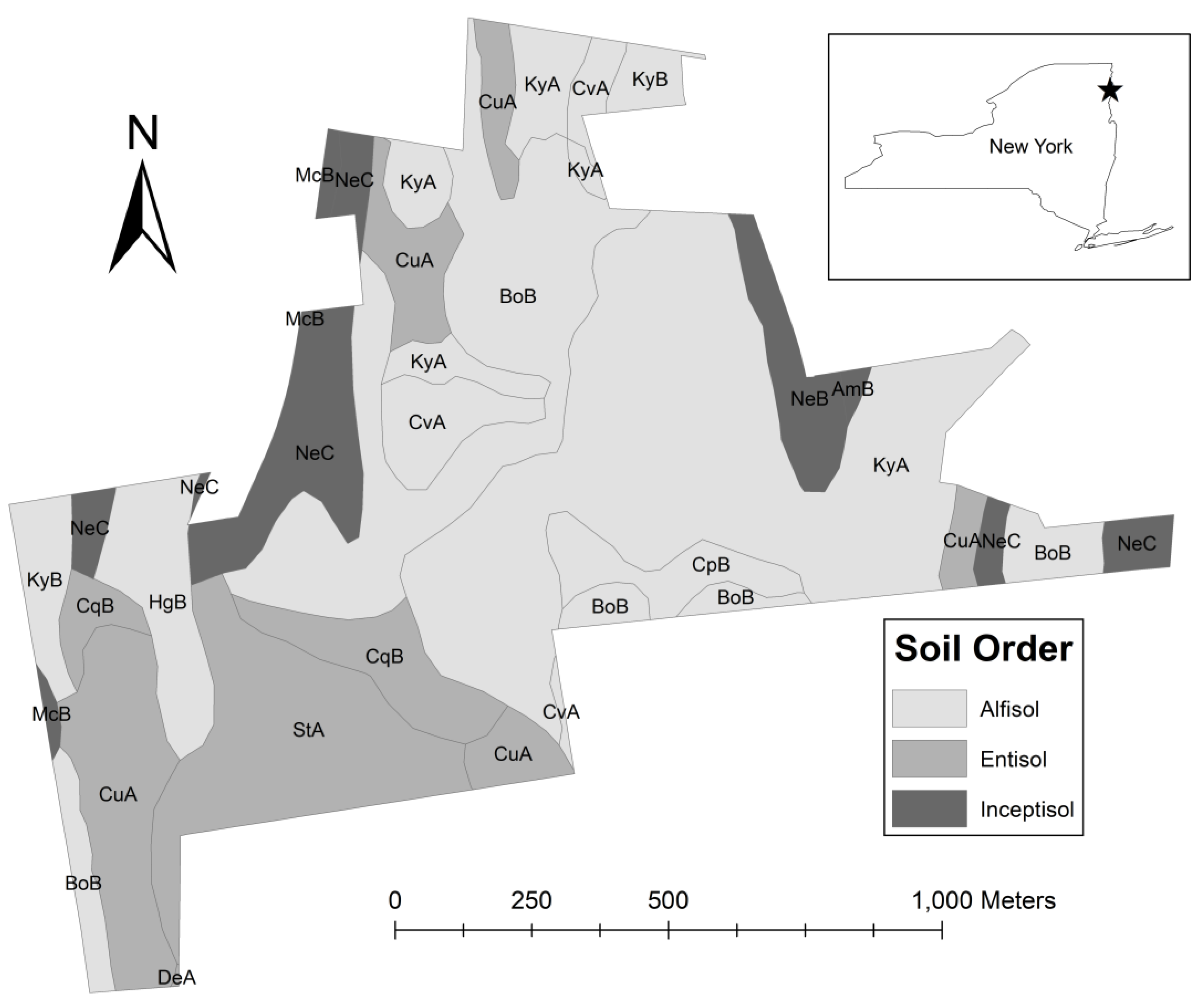
2.1. Study Area and Soil Analyses

Soil samples (n = 155) were collected from 53 soil cores at the Cornell University Willsboro Research Farm (Latitude/Longitude: 44.23, 73.23) near Willsboro, NY [18]. The 351-acre farm is located in the northeastern portion of New York State in the lacustrine plain near Lake Champlain with variable soils due to the differences caused by glacial deposits [18]. Average annual precipitation is 838 mm and with a 150 day growing season [18]. The soils present on the Willsboro Farm range from 0 to 15% slopes and consist of three soil orders. Alfisols, comprised of the soil series Bombay, Churchville, Covington, Howard, and Kingsbury, made up the largest number (n = 85) of soil samples collected within the study area (Figure 1). Entisols, comprised of the soil series Claverack, Cosad, Deerfield, and Stafford, contained the second highest number (n = 60) of soil samples collected within the study area (Figure 1). Inceptisols, comprised of the soil series Amenia, Massena, and Nellis, had the lowest number (n = 10) of soil samples collected within the study area (Figure 1). More detailed information regarding the soils found on the farm can be found in the Soil Survey of Essex County, NY, USA [19].

The collected soil samples were air dried, crumbled, and passed through a 2-mm sieve and then analyzed for SOC (%) and TN (%) using dry-combustion-mass spectrometry—a Robo-prep-Tracemass system (Europa Scientific, Cheshire, UK) [18]. TN (%) was not detectable in 10 of the Entisol soil samples. Depth was recorded for each sample as the lower depth of each horizon.

Table 1. Example of selected soil properties for Kingsbury (Alfisols), Cosad (Entisols), and Nellis (Inceptisols) soil series.

Sample ID	Munsell Color	Textural Class	SOC (%)	TN (%)	Depth (cm)	L*	a*	b*
Kingsbury silty clay loam
9	10YR 3/1	C	3.89	0.44	21	38.86	4.15	10.00
10	10YR 6/2	C	0.52	0.11	52	54.22	5.23	13.19
11	10YR 5/1	C	0.27	0.08	75	55.84	5.61	13.80
12	10YR 6/2	SiC	0.19	0.05	98	59.40	5.65	15.50
Cosad loamy fine sand
46	10YR 2/2	SL	2.48	0.21	14	42.49	4.56	10.41
47	10YR 4/1	CL	0.57	0.07	25	53.23	4.02	11.23
48	10YR 4/1	C	0.23	0.06	58	56.54	4.71	10.28
49	10YR 3/1	C	0.20	0.06	99	59.64	4.62	9.78
Nellis fine sandy loam
187	10YR 4/2	SL	4.09	0.31	24	47.62	6.78	13.62
188	10YR 5/6	FSL	0.50	0.04	35	58.93	9.33	22.54
189	7.5YR 4/6	FSL	0.24	0.02	49	54.90	11.04	24.42
190	7.5YR 4/6	SCL	0.33	0.03	75	54.34	8.48	21.21

Note: ID = identification; C = clay; SiC = silty clay; SL = sandy loam; CL = clay loam; FSL = fine sandy loam; SCL = silty clay loam; SOC = soil organic carbon; cm = centimeters; L* = lightness to darkness; a* = green to red; b* = blue to yellow.

shows an example of soil variables for Kingsbury (Alfisols), Cosad (Entisols), and Nellis (Inceptisols) soil series. For the present study, archived non-carbonated samples from the Willsboro Farm were analyzed dry for CIE L* a* b* color system (L* = lightness to darkness, a* = green to red, b* = blue to yellow) using a Nix Pro™ color sensor by placing a small (roughly 4 mm thick layer, 1.5 cm wide) amount of sample on a plate and the sensor’s viewing window placed directly on top to prevent any outside light interference. The rechargeable Nix Pro^TM has its own light emitting diode (LED) and is controlled through a mobile application and Bluetooth connection. Scan results are produced in a variety of color systems such as CIE L* a* b*, CMYK (cyan, magenta, yellow, black), and RGB (red, green, blue).

2.2. Development of Multiple Regression SOC and TN Prediction Models

Initial analyses indicated that a transformation of SOC (%) and total N (%) was necessary to account for curvature in residual plots when predicting these two variables using depth and CIE L* a* b* color variables. The natural log of SOC (%) and TN (%) (lnSOC (%) and lnTN (%), respectively) were considered as the dependent variables in separate models. Additionally, high Pearson’s correlation coefficients were found between the color variables (

Table 2. Pearson correlation (r) values among soil variables for the lnSOC (%) analysis for all soil orders, Alfisols, and Entisols for the soil set samples.

Variable	lnSOC (%)	Depth (cm)	L*	a*	b*
All soil samples (n = 155)
lnSOC (%)	---	−0.78 ***	−0.78 ***	−0.33 ***	−0.54 ***
lnTN (%)		−0.63 ***	−0.79 ***	−0.57 ***	−0.74 ***
Depth (cm)		---	0.62 ***	0.12	0.27 ***
L*			---	0.40 ***	0.64 ***
a*				---	0.90 ***
b*					---
Alfisols (n = 85)
lnSOC (%)	---	−0.79 ***	−0.79 ***	−0.11	−0.36 *
lnTN (%)		−0.64 ***	−0.78 ***	−0.41 ***	−0.62 ***
Depth (cm)		---	0.63 ***	−0.09	0.12
L*			---	0.30 **	0.59 ***
a*				---	0.86 ***
b*					---
Entisols (n = 60)
lnSOC (%)	---	−0.76 ***	−0.77 ***	−0.37 **	−0.59 ***
lnTN (%)		−0.62 ***	−0.79 ***	−0.56 ***	−0.76 ***
Depth (cm)		---	0.63 ***	0.25	0.37 **
L*			---	0.39 **	0.63 ***
a*				---	0.91 ***
b*					---

Note: Significance defined as * (p-value < 0.05), ** (p-value < 0.01), *** (p-value < 0.001). Inceptisols samples included within all soil samples set (n = 156). lnSOC = natural log of soil organic carbon; lnTN = natural log of total nitrogen; cm = centimeters; L* = lightness to darkness; a* = green to red; b* = blue to yellow.

), and the variance inflation factor indicated that either a* or b* be excluded from the models predicting the two dependent variables. Because b* had a higher correlation with the dependent variables than a*, a* was excluded from the regression models.

Because the soil samples were obtained from 53 soil cores in the study region, a mixed effects model was fit to examine the variation between soil cores in each model predicting lnSOC (%) and lnTN (%). For both dependent variables, the soil core variation was not significant (p > 0.05). Additionally, the fitted models had similar parameter estimates regardless of whether a mixed effects model or a least squares model was used to estimate the parameters.

For prediction models of all soil samples regardless of soil order, approximately 70% (n = 108) of the samples were randomly selected to be used as the training set and the remaining 30% (n = 47) of the samples were set aside for cross validation. Regression models were fit using either the lnSOC (%) or the lnTN (%) as the dependent variable and soil horizon lower depth, L*, and b* as the independent variables. Assessments of R², adjusted R² (Adj. R²), root mean squared error (RMSE), and p-values were considered for model fit and significance. For each of the dependent variables, two models were fit including one with sample horizon depth and color variables as predictor variables and one without sample horizon depth (i.e., only soil color variables were included as predictors). A level of significance of 0.05 was used for all tests of significance.

Regression models were also fit for data within the soil orders present on the Willsboro Farm: Alfisols (n = 60, 70% of total n = 85) and Entisols (n = 42, 70% of total n = 60). A regression analysis and cross-validated analysis for Inceptisols (n = 10) alone was not conducted due to limited sample size.

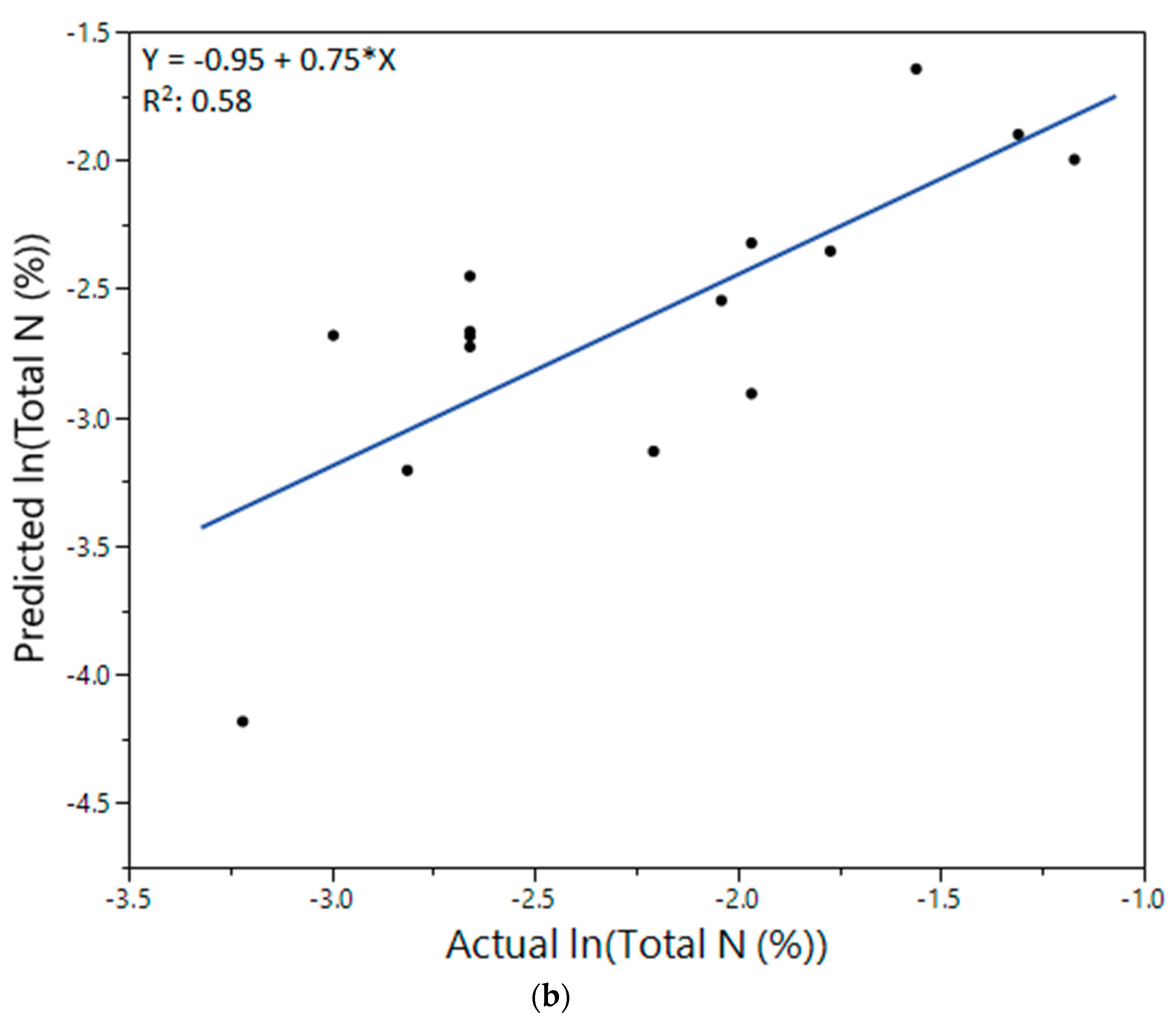
2.3. Validation of SOC and TN Prediction Models

Thirty percent of all soil samples (n = 47), of Alfisols (n = 26), and of Entisols (n = 18) were randomly selected to be used as a validation set. Regression models that were developed to predict the lnSOC (%) or lnTN (%) were used to predict these values using the soil horizon depth and color variable observations in the validation set. The mean squared prediction error (MSPE) was calculated for each model; smaller MSPE values indicate more accurate predictions. All statistical analyses were performed using JMP^®, Version 13 Pro. [20] and IBM SPSS Statistics for Windows, Version 24.0 [21].

3. Results and Discussions

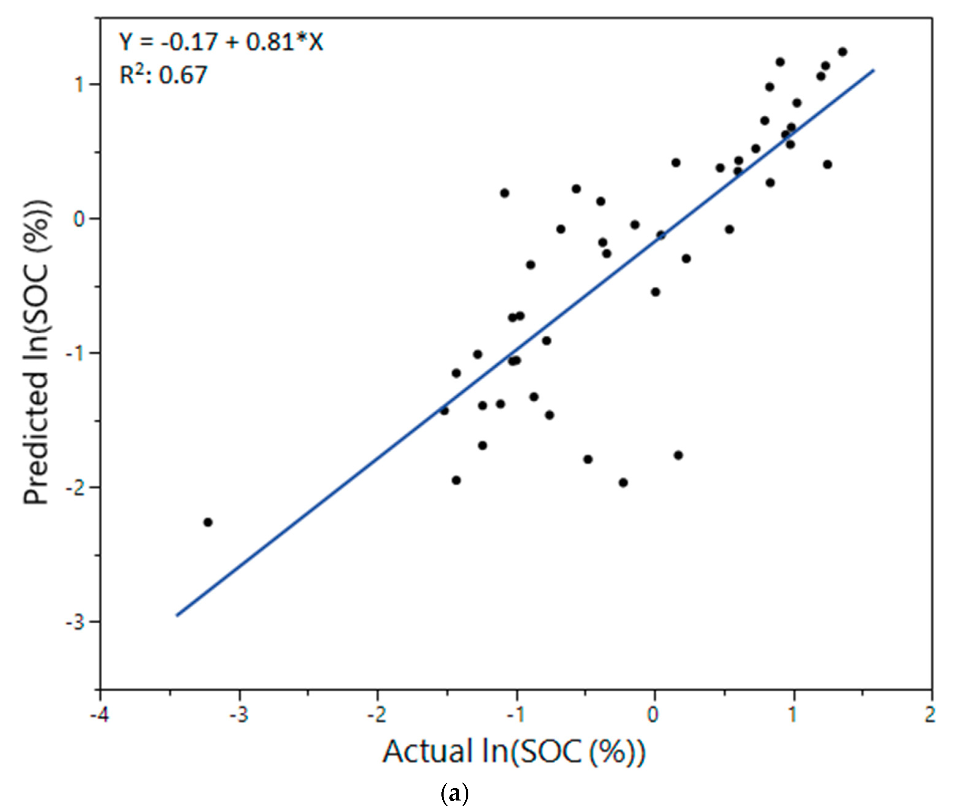
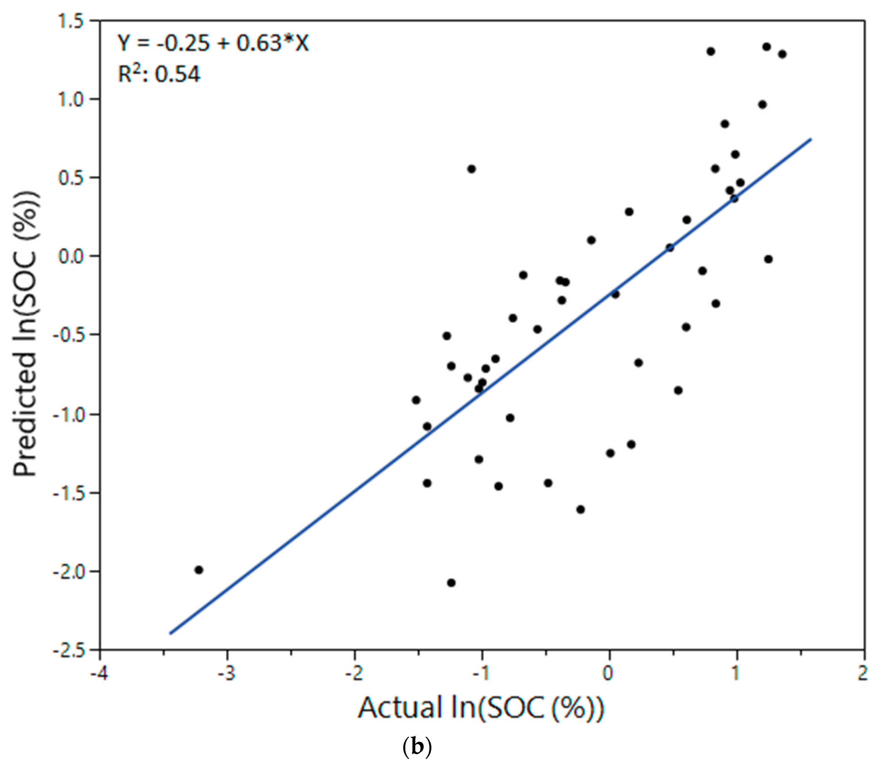
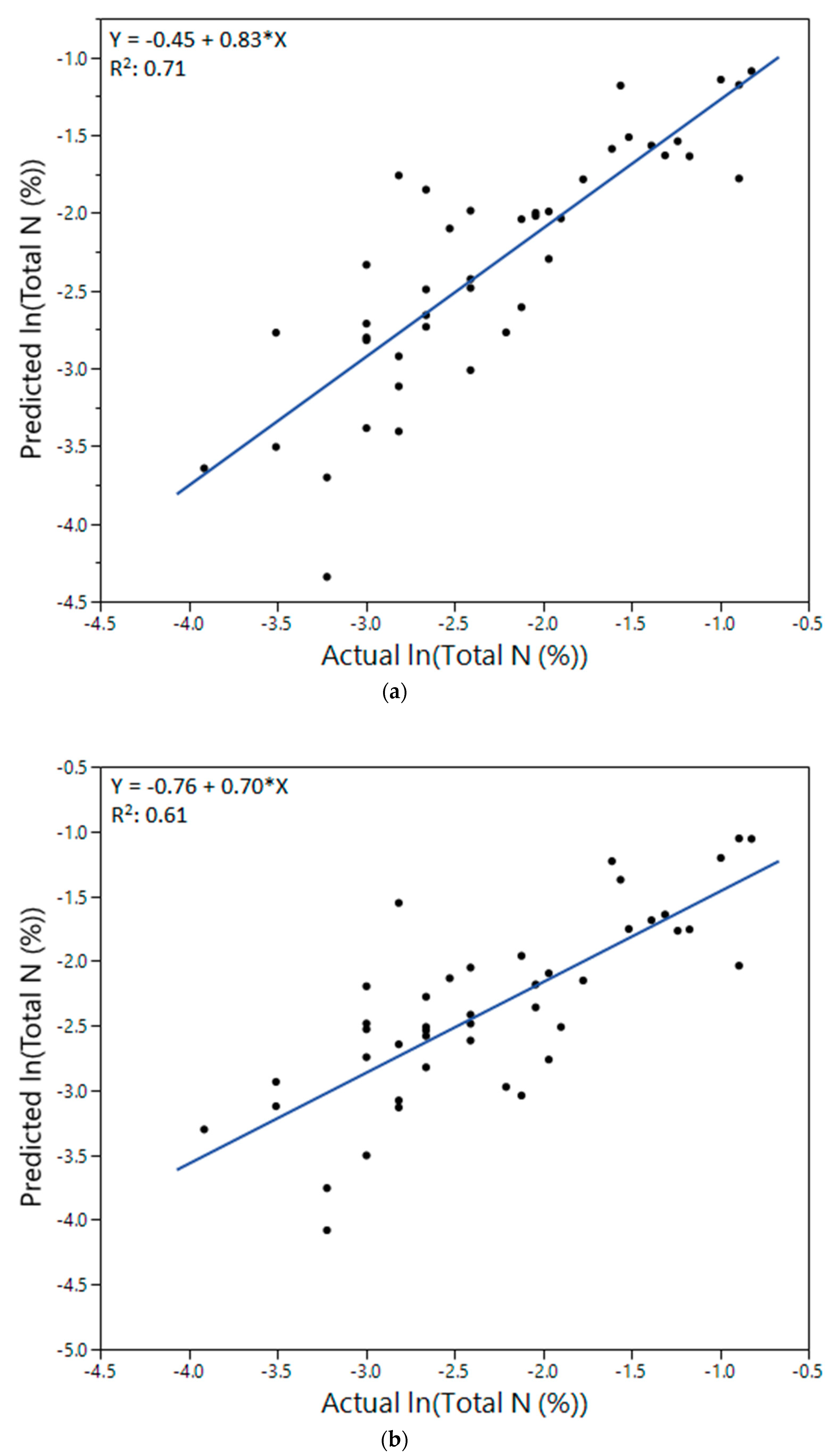
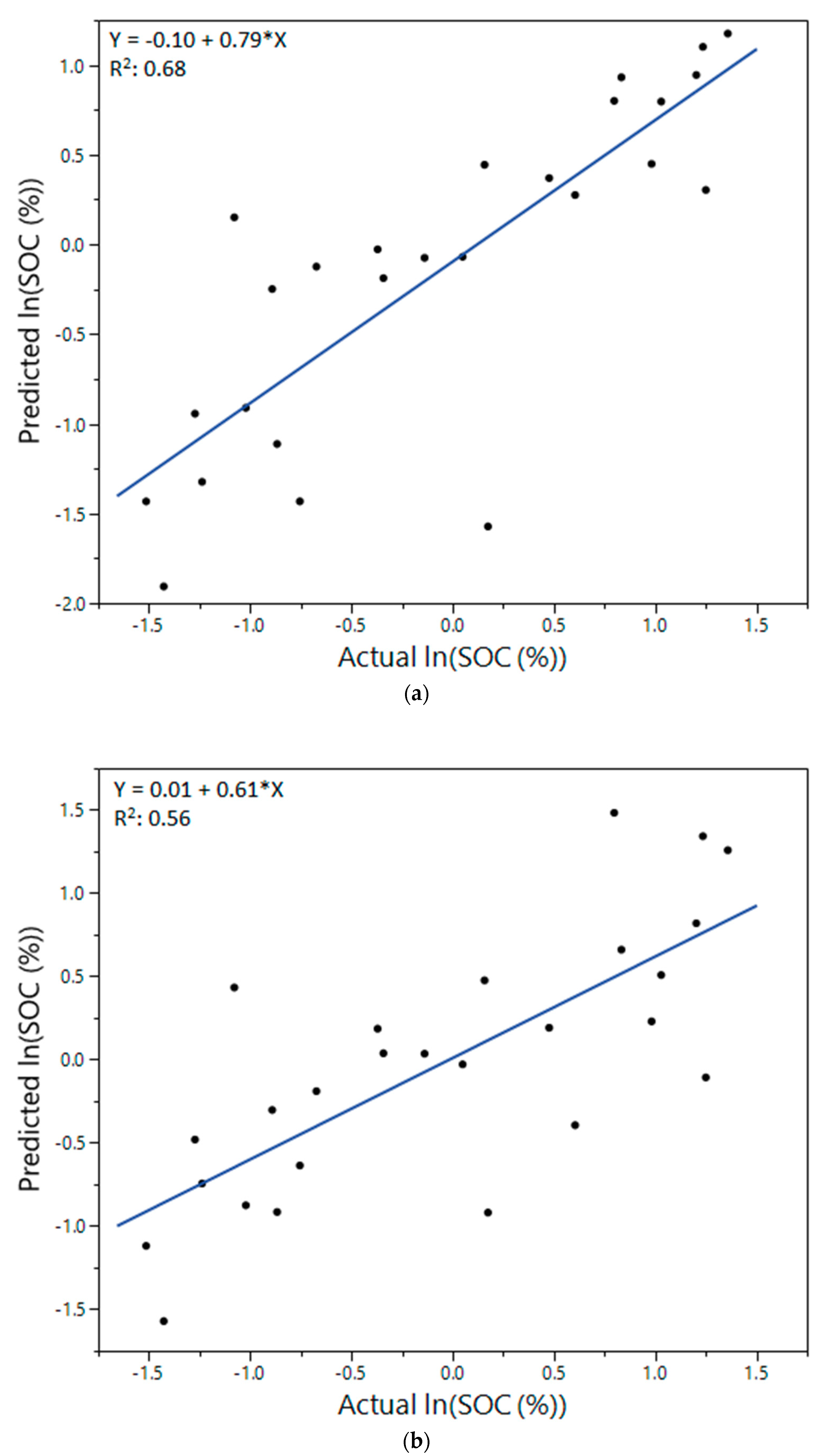
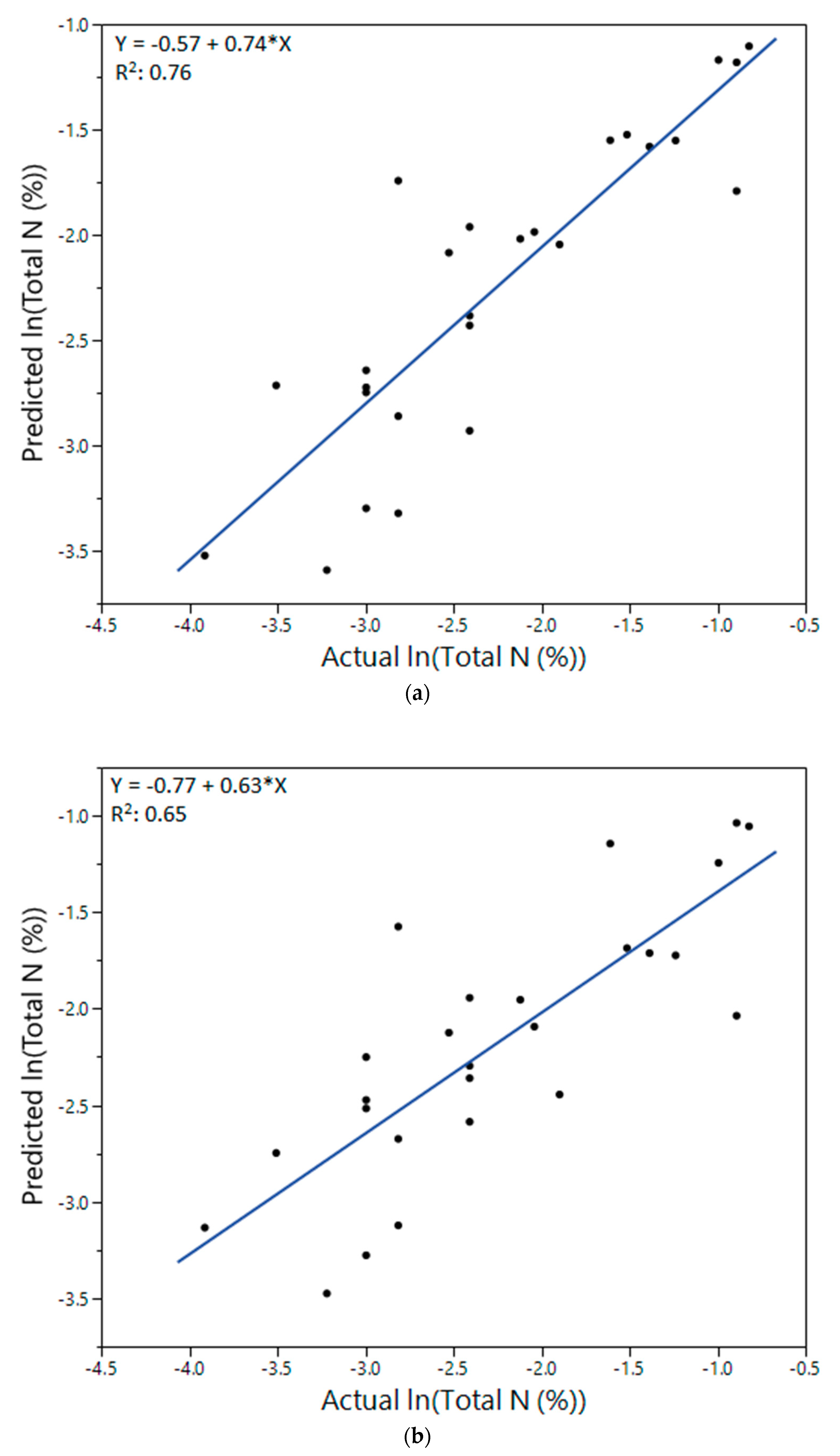
3.1. Prediction Models for lnSOC and lnTN for All Soil Orders

Separate multiple regression analyses were conducted on 70% (n = 109) of all soil samples taken together using sample horizon lower depth together with color variables, and using color variables only, as predictors to predict lnSOC (%) and lnTN (%). The color variable a* was excluded from analysis due to its large correlation with the other predictors. The removal of a* may also be beneficial because iron oxides, which are red in color, tends to form complexes with organic matter in soil [22]. This interaction may interfere with soil color analysis and the accurate prediction of SOC in soil. The lnSOC (%) prediction model, which included depth and color variables, indicated that depth, L*, b* were significant predictors of lnSOC (%) (

Table 3. Variable estimates and ANOVA results for final prediction models using depth (cm) and color variables, and color variables alone, to predict lnSOC (%).

Model	Variable	Variable Estimate	Variable p-Value	Model p-Value	RMSE	R2	Adj. R2	MSPE
Depth and Color Variables
All soils	Constant	4.49	<0.001	<0.001	0.51	0.81	0.80	0.36
	Depth (cm)	−0.02	<0.001
	L*	−0.06	<0.001
	b*	−0.04	0.003
Alfisols	Constant	4.47	<0.001	<0.001	0.42	0.81	0.80	0.30
	Depth (cm)	−0.02	<0.001
	L*	−0.07	<0.001
	b*	−0.01	0.689
Entisols	Constant	4.45	<0.001	<0.001	0.61	0.76	0.74	0.48
	Depth (cm)	−0.02	<0.001
	L*	−0.06	0.002
	b*	−0.04	0.051
Color Variables
All soils	Constant	6.13	<0.001	<0.001	0.68	0.65	0.64	0.71
	L*	−0.12	<0.001
	b*	−0.02	0.281
Alfisols	Constant	6.15	<0.001	<0.001	0.56	0.67	0.66	0.39
	L*	−0.14	<0.001
	b*	0.05	0.073
Entisols	Constant	5.41	<0.001	<0.001	0.75	0.62	0.60	0.69
	L*	−0.10	<0.001
	b*	0.04	0.146

Note: MSPE calculated from predicted and actual observations of the lnSOC (%) for the validation set. All other values determined through regression analysis. RMSE = root mean squared error; R² = coefficient of determination; Adj. R² = adjusted coefficient of determination; MSPE = mean squared prediction error; cm = centimeters; L* = lightness to darkness; b* = blue to yellow.

). Cross-validation resulted in a MSPE of 0.36 (R² = 0.67; Figure 2a, Table 3). The lnSOC (%) prediction model, which included only color variables, indicated that L* was a significant predictor of lnSOC (%) while b* was not (Table 3). Cross-validation resulted in a MSPE of 0.71 (R² = 0.54; Figure 2b, Table 3). The results suggest that including sample horizon lower depth accounts for more variability in lnSOC (%). This can be seen by a larger R² value and smaller RMSE and MSPE values for the model which included depth. In fact, the prediction error (MSPE) nearly doubled when depth was excluded. In both models, L* is shown to be a significant predictor of lnSOC (%) which agrees with the other studies which use soil color to predict SOC [13,23].

The lnTN (%) prediction model, which included depth and color variables, indicated that depth, L*, and b* were significant predictors of lnTN (%) (

Table 4. Variable estimates and ANOVA results for final prediction models using depth (cm) and color variables, and color variables alone, to predict lnTN (%).

Model	Variable	Variable Estimate	Variable p-Value	Model p-Value	Root MSE	R2	Adj. R2	MSPE
Depth and Color Variables
All soils	Constant	1.73	<0.001	<0.001	0.46	0.76	0.75	0.18
	Depth (cm)	−0.01	<0.001
	L*	−0.04	<0.001
	b*	−0.09	<0.001
Alfisols	Constant	1.68	0.002	<0.001	0.42	0.73	0.71	0.17
	Depth (cm)	−0.01	<0.001
	L*	−0.04	0.005
	b*	−0.08	<0.001
Entisols	Constant	1.46	0.063	<0.001	0.51	0.72	0.69	0.23
	Depth (cm)	−0.01	0.015
	L*	−0.04	0.018
	b*	−0.08	<0.001
Color Variables
All soils	Constant	2.75	<0.001	<0.001	0.53	0.67	0.67	0.25
	L*	−0.08	<0.001
	b*	−0.08	<0.001
Alfisols	Constant	2.69	<0.001	<0.001	0.47	0.65	0.64	0.26
	L*	−0.08	<0.001
	b*	−0.05	0.047
Entisols	Constant	2.08	0.012	<0.001	0.55	0.65	0.63	0.32
	L*	−0.07	<0.001
	b*	−0.08	0.001

Note: MSPE calculated from predicted and actual lnTN (%) for the validation set. All other values determined through regression analysis. RMSE = root mean squared error; R² = coefficient of determination; Adj. R² = adjusted coefficient of determination; MSPE = mean squared prediction error; cm = centimeters; L* = lightness to darkness; b* = blue to yellow.

). Cross-validation resulted in a MSPE of 0.18 (R² = 0.71; Figure 3a, Table 4). The lnTN (%) prediction models, which included only color variables, indicated that L* and b* were both significant predictors of lnTN (%) (Table 4). Cross-validation resulted in a MSPE of 0.248 (R² = 0.61; Figure 3b, Table 4). Depth accounts for more variability in lnTN (%) when included in the model, resulting in a larger R² value. Interestingly, b* is a significant predictor of lnTN (%), but not for lnSOC (%) for all soil samples combined. Further investigation into the relationship between how blue or yellow (b*) a soil may appear and TN content may help to develop stronger TN prediction models.

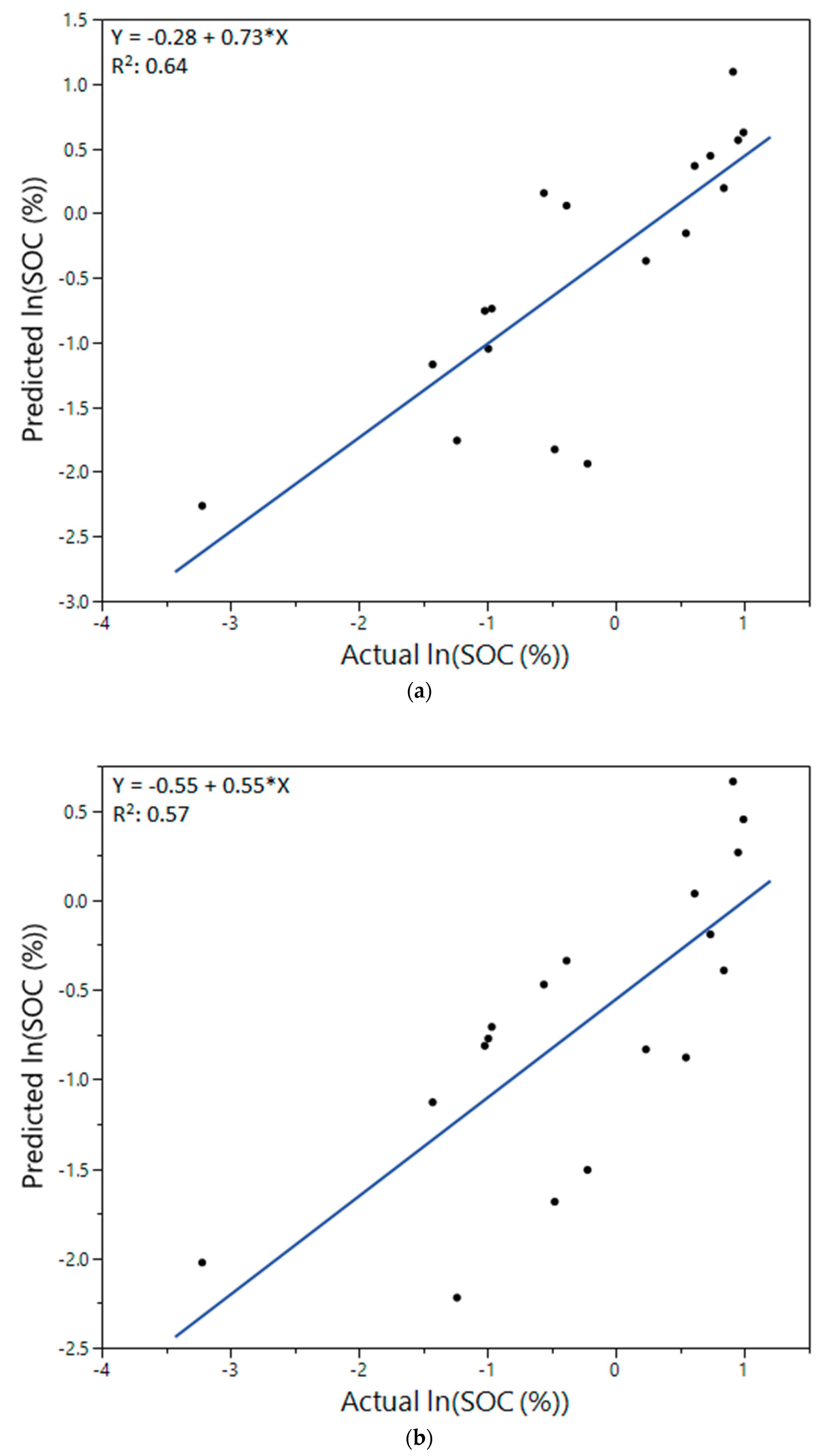
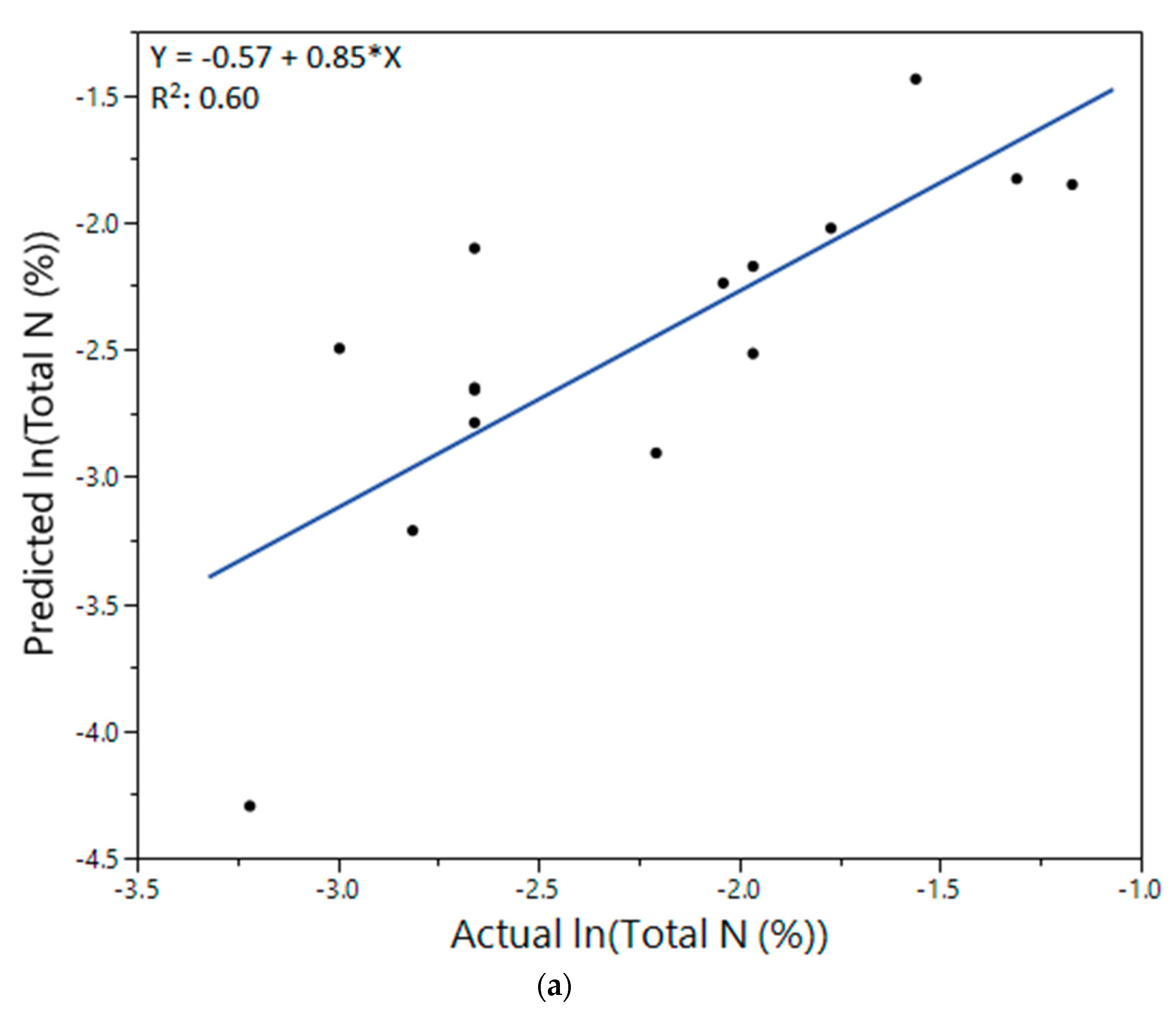
3.2. Prediction Models for lnSOC and lnTN by Soil Order: Alfisols, Entisols

Soil-based management often relies on existing soil survey maps which provide soil order information as a basis for separating soil properties within the landscape. Therefore, it is important to examine the color sensor prediction models for SOC and TN by soil order.

Separate multiple regression analyses were conducted on 70% (n = 60) of Alfisols using sample horizon lower depth together with color variables, and using color variables only, as predictors to predict lnSOC (%) and lnTN (%). Again, the color variable a* was excluded from analysis due to its large correlation with the other predictors. The lnSOC (%) prediction model, which included depth and color variables, indicated that depth and L* were significant predictors of lnSOC (%) but b* was not (Table 3). Cross-validation resulted in a MSPE value of 0.30 (R² = 0.68; Figure 4a, Table 3). The lnSOC (%) prediction model, which included only color variables, indicated that L* was a significant predictor of lnSOC (%) and b* was marginally insignificant (Table 3). Cross-validation resulted in a MSPE value of 0.39 (R² = 0.56; Figure 4b, Table 3). When the analysis focuses on Alfisols alone, depth still appears to account for large amount of variability in lnSOC (%) as shown by a larger R² value for the model which included depth as a predictor. The RMSE increased when depth was removed, however, the MSPE value did not seem to increase by much. However, R² values for both models were similar to those produced by the logarithmic transformation of SOC prediction models developed by [23] which ranged from 0.53 to 0.84.

The lnTN (%) prediction model, which included depth and color variables, indicated that depth, L*, and b* were significant predictors of lnTN (%) (Table 4). Cross-validation resulted in a MSPE value of 0.17 (R² = 0.76; Figure 5a, Table 4). The lnTN (%) prediction model, which included only color variables, indicated that L* and b* were significant predictors of lnTN (%) (Table 4). Cross-validation resulted in a MSPE value of 0.26 (R² = 0.65; Figure 5b, Table 4). Again, b* did not prove to be a significant predictor of lnSOC (%), but it did for lnTN (%) for Alfisols.

Separate multiple regression analyses were conducted on 70% (n = 42) of Entisols using sample horizon lower depth together with color variables, and using color variables only, as predictors to predict lnSOC (%) and lnTN (%). Again, the color variable a* was excluded from analysis due to its large correlation with the other predictors. The lnSOC (%) prediction model, which included depth and color variables, indicated that depth and L* were significant predictors of lnSOC (%) while b* was marginally insignificant (Table 3). Cross-validation resulted in a MSPE of 0.48 (R² = 0.64; Figure 6a, Table 3). The lnSOC (%) prediction model, which included color variables only, indicated that L* was a significant predictor of lnSOC (%) while b* was not (Table 3). Cross-validation resulted in a MSPE of 0.69 (R² = 0.57; Figure 6b, Table 3). The lnTN (%) prediction model, which contained depth and color variables, indicated that depth, L*, and b* were significant predictors of lnTN (%) (Table 4). Cross-validation resulted in a MSPE value of 0.23 (R² = 0.60; Figure 7a, Table 4). The lnTN (%) prediction model, which contained color variables only, indicated that L* and b* were significant predictors of lnTN (%) (RMSE = 0.55, R² = 0.65, Adj. R = 0.63; Table 4). Cross-validation resulted in a MSPE value of 0.316 (R² = 0.58; Figure 7b, Table 4).

As expected, depth improved the R² when included in the models for Entisols and the color variable b* was again a significant predictor of lnTN (%) but not lnSOC (%). Parent material, land-use, and vegetation may also play a key role in soil color variables. For example, when plant roots die off and decompose into organic matter in soil, the soil color may appear darker [24]. Prediction models may be different among soil orders as parent materials, land use, climate, and other factors may affect SOC and TN content, or soil color [25]. This study did not have sufficient available land use information to consider that as a factor. Color and depth data for soil samples within the order Alfisols produced the least accurate models indicating that there may be influences not considered in this analysis. Alfisols are older, more developed soils than Entisols which may explain the variability in SOC as well as TN content [26]. Given that SOC and TN are often strongly correlated to one another, it would be expected that the variables included within a SOC prediction model would be similar to those included in a TN prediction model [27]. Past studies have shown that a soil’s lightness or darkness (L*) are a key factor in determining SOC (%) [13]. The results of this study suggest that a soil’s color range from yellow to blue (b*) may be a more important indicator of TN (%) which may provide key insight into how nitrogen content affects soil color. Further study of this trend may help to develop more accurate nitrogen prediction models.

Benefits of pre-analysis transformations, including logarithmic transformations of SOC and TN variables for improving model fit and prediction accuracy, were previously documented [28]. Combining all soil order samples produced effective SOC and TN prediction models, however RMSE was higher for this set than it was for Alfisols alone and was comparable to Entisols for a few models. It is important to note that Inceptisols samples were not separately tested using regression analysis due to the small sample size, but were included within the model development for all soil order samples. While these samples may have introduced unwanted error within the models, the resulting R², RMSE, and MSPE values suggest only a small impact and the regression models were still efficient at predicting lnSOC and lnTN in soil.

Including depth in each model improved model fit and prediction accuracy and therefore depth is a useful predictor of SOC and TN within models. Regardless of the improvement the inclusion of depth makes to a model, the R² values which resulted from the prediction models containing only color variables are comparable to previous SOC prediction models [23]. This would suggest that there is great potential for further development of SOC and TN prediction models based solely on soil color. Sensor measurements are rapid and can be linked to GPS location for creation of high spatial density maps of estimated SOC and TN at relatively low cost for smaller agricultural producers that have not had access to this type of technology. This new sensor technology could also be utilized for precision agriculture regardless of farm size (e.g., linking sensor measurements to different management zones).

4. Conclusions

This research demonstrates use of low-cost wireless color sensor technology to predict SOC and TN content in variable, glaciated soils located on the Willsboro Farm in Upstate New York. A soil’s lightness to darkness variable (L*) proved significant in predicting SOC content while blue to yellow (b*) was significant predictor of TN. Including depth in each prediction model improved model fit and prediction accuracy, and reduced the MSPE. Further research into the effects of soil order on prediction efficiency may help to develop stronger or more universal prediction models in the future. The correlation between a* (green to red) and b* (blue to yellow) should be further investigated as well as their relationship with SOC and TN. Finally, a larger data set may be beneficial in developing stronger prediction models which include only soil color variables as predictors of SOC and TN. Sensor technology offers a reliable and inexpensive means of gathering soil data and has the potential to be used in soil quality assessment. The portability and accuracy of the Nix Pro^TM color system may prove beneficial to soil science as a means of rapid SOC and TN quantification. This new sensor technology could also be utilized for precision agriculture (e.g., linking sensor measurements to variable-rate fertilizer application software). In addition, such an inexpensive, rapid analysis method could allow for the continuous collection of SOC and TN data on a higher spatial and temporal density which could assist in monitoring soil changes under different land uses.

References

1. Khormali, F.; Ajami, M.; Ayoubi, S.; Srinivasarao, C.; Wani, S.P. Role of deforestation and hillslope position on soil quality attributes of loess-derived soils in Golestan Province, Iran. Agric. Ecosyst. Environ. 2009, 134, 178–189. [Google Scholar] [CrossRef]
2. Ajami, M.; Heidari, A.; Khormali, F.; Gorji, M.; Ayoubi, S. Environmental factors controlling soil organic carbon storage in loess soils of a subhumid region, Northern Iran. Geoderma 2016, 281, 1–10. [Google Scholar] [CrossRef]
3. Ayoubi, A.; Khormali, F.; Sahrawat, K.L.; Rodrigues de Lima, A.C. Assessing impacts of land use change on soil quality indicators in a loessial soil in Golestan Province, Iran. J. Agric. Sci. Technol. 2011, 13, 727–742. [Google Scholar]
4. Fernández-Martínez, M.; Vicca, S.; Janssens, I.A.; Sardans, J.; Luyssaert, S.; Campioli, M.; Chapin, F.S., III; Ciais, P.; Malhi, Y.; Obersteiner, M.; et al. Nutrient availability as the key regulator of global forest carbon balance. Nat. Clim. Chang. 2014, 4, 471–476. [Google Scholar] [CrossRef]
5. Madhavan, D.B.; Baldock, J.A.; Read, Z.J.; Murphy, S.C.; Cunningham, S.C.; Perrings, M.P.; Herrmann, T.; Lewis, T.; Cavagnaro, T.R.; England, J.R.; et al. Rapid prediction of particulate, humus and resistant fractions of soil organic carbon in reforested lands using infrared spectroscopy. J. Environ. Manag. 2017, 193, 290–299. [Google Scholar] [CrossRef] [PubMed]
6. Viscarra Rossel, R.A.; Fouad, Y.; Walter, C. Using a digital camera to measure soil organic carbon and iron contents. Biosyst. Eng. 2008, 100, 149–159. [Google Scholar] [CrossRef]
7. Nocita, M.; Stevens, A.; Toth, G.; Panagos, P.; van Wesemael, B.; Montanarella, L. Prediction of soil organic carbon content by diffuse reflectance spectroscopy using a local partial least square regression approach. Soil Biol. Biochem. 2014, 68, 337–347. [Google Scholar] [CrossRef]
8. Aitkenhead, M.J.; Donnelly, D.; Sutherland, L.; Miller, D.G.; Coull, M.C.; Black, H.I.J. Predicting Scottish topsoil organic matter content from colour and environmental factors. Eur. J. Soil Sci. 2015, 66, 112–120. [Google Scholar] [CrossRef]
9. Wang, C.; Feng, M.; Yang, W.; Ding, G.; Wang, H.; Li, Z.; Sun, H.; Shi, C. Use of spectral character to evaluate soil organic matter. Soil Sci. Soc. Am. J. 2016, 80, 1078–1088. [Google Scholar] [CrossRef]
10. Deiss, L.; Franzluebbers, A.J.; de Moraes, A. Soil texture and organic carbon fractions predicted from near-infrared spectroscopy and geostatistics. Soil Sci. Soc. Am. J. 2017, 81, 1222–1234. [Google Scholar] [CrossRef]
11. Vagen, T.G.; Winowiecki, L.A.; Tondoh, J.E.; Desta, L.T.; Gumbricht, T. Mapping of soil properties and land degradation risk in Africa using MODIS reflectance. Geoderma 2016, 262, 216–225. [Google Scholar] [CrossRef]
12. Harvey, O.R.; Herbert, B.E.; Harris, J.P.; Stiffler, E.A.; Crenwelge, J. A new spectrophotometric method for rapid semiquantitative determination of soil organic carbon. Soil Sci. Soc. Am. J. 2009, 73, 822–830. [Google Scholar] [CrossRef]
13. Liles, G.C.; Beaudette, D.E.; O’Green, A.T.; Horwath, W.R. Developing predictive soil C models for soils using quantitative color measurements. Soil Sci. Soc. Am. J. 2013, 77, 2173–2181. [Google Scholar] [CrossRef]
14. Stiglitz, R.; Mikhailova, E.; Post, C.; Schlautman, M.; Sharp, J. Evaluation of an inexpensive sensor to measure soil color. Comput. Electron. Agric. 2016, 121, 141–148. [Google Scholar] [CrossRef]
15. Stiglitz, R.; Mikhailova, E.; Post, C.; Schlautman, M.; Sharp, J. Using an inexpensive color sensor for rapid assessment of soil organic carbon. Geoderma 2016, 286, 98–103. [Google Scholar] [CrossRef]
16. Mikhailova, E.A.; Stiglitz, R.Y.; Post, C.J.; Schlautman, M.A.; Sharp, J.L.; Gerard, P.D. Predicting soil organic carbon and total nitrogen in the Russian Chernozem from depth and wireless color sensor measurements. Eurasian Soil Sci. 2017, 50, 1414–1419. [Google Scholar] [CrossRef]
17. Aitkenhead, M.; Cameron, C.; Gaskin, G.; Choisy, B.; Coull, M.; Black, H. Digital RGB photography and visible-range spectroscopy for soil composition analysis. Geoderma 2018, 313, 265–275. [Google Scholar] [CrossRef]
18. Mikhailova, E.A.; Van Es, H.M.; Lucey, R.F.; DeGloria, S.D.; Schwager, S.J.; Post, C.J. Soil Characterization Data for Selected Pedons from the Willsboro Farm, Essex County, New York; Research Series R96-5; Department of Soil, Crop, and Atmospheric Sciences, Cornell University: Ithaca, NY, USA, 1996; p. 14853. [Google Scholar]
19. Soil Survey of Essex County, New York. Available online: https://www.nrcs.usda.gov/Internet/FSE_MANUSCRIPTS/new_york/essexNY2010/Essex_NY.pdf (accessed on 26 September 2017).
20. JMP®; Version 13 Pro; SAS Institute Inc.: Cary, NC, USA, 2007.
21. IBM SPSS Statistics for Windows; Version 24.0; IBM Corp: Armonk, NY, USA, 2016.
22. Neubauer, E.; Schenkeveld, W.D.C.; Plathe, K.L.; Rentenberger, C.; von der Kammer, F.; Kraemer, S.M.; Hofmann, T. The influence of pH on iron speciation in podzol extracts: Iron complexes with natural organic matter, and iron mineral nanoparticles. Sci. Total Environ. 2013, 461, 108–116. [Google Scholar] [CrossRef] [PubMed]
23. Wills, S.A.; Burras, C.L.; Sandor, J.A. Prediction of soil organic carbon content using field and laboratory measurements of soil color. Soil Sci. Soc. Am. J. 2007, 71, 380–388. [Google Scholar] [CrossRef]
24. Pereira, P.; Ubeda, X.; Mataix-Solera, J.; Oliva, M.; Novara, A. Short-term changes in soil Munsell colour value, organic matter content and soil water repellency after a spring grassland fire in Lithuania. Solid Earth 2014, 5, 209–225. [Google Scholar] [CrossRef] [Green Version]
25. Aitkenhead, M.J.; Coull, M.C.; Towers, W.; Hudson, G.; Black, H.I.J. Predicting soil chemical composition and other soil parameters from field observations using a neural network. Comput. Electron. Agric. 2012, 82, 108–116. [Google Scholar] [CrossRef]
26. Bockheim, J.G.; Gennadiyev, A.N.; Hartemink, A.E.; Brevik, E.C. Soil-forming factors and Soil Taxonomy. Geoderma 2014, 226, 231–237. [Google Scholar] [CrossRef]
27. Anderson, T.; Domsch, K.H. Ratios of microbial biomass carbon to total organic carbon in arable soils. Soil Biol. Biochem. 1989, 21, 471–479. [Google Scholar] [CrossRef]
28. Vasques, G.M.; Grunwald, S.; Sickman, J.O. Comparison of multivariate methods for inferential modeling of soil carbon using visible/near-infrared spectra. Geoderma 2008, 146, 14–25. [Google Scholar] [CrossRef]
Figure 1. Map showing the extent of the soil series separated by soil order (soil series, map unit symbol) according to the U.S. Soil Taxonomy: Alfisols (Bombay gravelly loam, 3 to 8 percent slope, BoB; Churchville loam, 2 to 8 percent slopes, CpB; Covington clay, 0 to 3 percent slopes, CvA; Howard gravelly loam, 2 to 8 percent slopes, HgB; Kingsbury silty clay loam, 0 to 3 percent slopes, KyA; Kingsbury silty clay loam, 3 to 8 percent slopes, KyB); Entisols (Claverack loamy fine sand, 3 to 8 percent slopes, CqB; Cosad loamy fine sand, 0 to 3 percent slopes, CuA; Deerfield loamy sand, 0 to 3 percent slopes, DeA; Stafford fine sandy loam, 0 to 3 percent slopes, StA); and Inceptisols (Amenia fine sandy loam, 2 to 8 percent slopes, AmB; Massena gravelly silt loam, 3 to 8 percent slopes, McB; Nellis fine sandy loam, 3 to 8 percent slopes, NeB; Nellis fine sandy loam, 8 to 15 percent slopes, NeC).
Agronomy 08 00212 g001
Figure 2. Plots of predicted lnSOC (%) content versus actual lnSOC (%) content for validation data sets for dry soil samples of all soil orders using (a) models which included depth and color variables (p-value < 0.001), and (b) models which included only color variables as predictors (p-value < 0.001).
Agronomy 08 00212 g002aAgronomy 08 00212 g002b
Figure 3. Plots of predicted lnTN (%) versus actual lnTN (%) for validation data sets for dry soil samples of all soil orders using (a) models which included depth and color variables (p-value < 0.001), and (b) models which included only color variables as predictors (p-value < 0.001).
Agronomy 08 00212 g003
Figure 4. Plots of predicted lnSOC (%) content versus actual lnSOC (%) content for validation data sets for dry soil samples of Alfisols using (a) models which included depth and color variables (p-value < 0.001), and (b) models which included only color variables as predictors (p-value < 0.001).
Agronomy 08 00212 g004
Figure 5. Plots of predicted lnTN (%) versus actual lnTN (%) for validation data sets for dry soil samples of Alfisols using (a) models which included depth and color variables (p-value < 0.001), and (b) models which included only color variables as predictors (p-value < 0.001).
Agronomy 08 00212 g005
Figure 6. Plots of predicted lnSOC (%) content versus actual lnSOC (%) content for validation data sets for dry soil samples of Entisols using (a) models which included depth and color variables (p-value < 0.001), and (b) models which included only color variables as predictors (p-value < 0.001).
Agronomy 08 00212 g006
Figure 7. Plots of predicted lnTN (%) versus actual lnTN (%) for validation data sets for dry soil samples of Entisols using (a) models which included depth and color variables (p-value < 0.001), and (b) models which included only color variables as predictors (p-value < 0.001).
Agronomy 08 00212 g007aAgronomy 08 00212 g007b