Generating Improved Experimental Designs with Spatially and Genetically Correlated Observations Using Mixed Models

Abstract

The aim of this study was to generate and evaluate the efficiency of improved field experiments while simultaneously accounting for spatial correlations and different levels of genetic relatedness using a mixed models framework for orthogonal and non-orthogonal designs. Optimality criteria and a search algorithm were implemented to generate randomized complete block (RCB), incomplete block (IB), augmented block (AB) and unequally replicated (UR) designs. Several conditions were evaluated including size of the experiment, levels of heritability, and optimality criteria. For RCB designs with half-sib or full-sib families, the optimization procedure yielded important improvements under the presence of mild to strong spatial correlation levels and relatively low heritability values. Also, for these designs, improvements in terms of overall design efficiency (ODE%) reached values of up to 8.7%, but these gains varied depending on the evaluated conditions. In general, for all evaluated designs, higher ODE% values were achieved from genetically unrelated individuals compared to experiments with half-sib and full-sib families. As expected, accuracy of prediction of genetic values improved as levels of heritability and spatial correlations increased. This study has demonstrated that important improvements in design efficiency and prediction accuracies can be achieved by optimizing how the levels of a treatment are assigned to the experimental units.

1. Introduction

Designing an experiment is an essential stage in any research settings. Important planning decisions are taken in order to choose the most appropriate layout out of an array of design alternatives. Generating experimental designs relies on three basic principles: randomization, replication and blocking [1,2]. Replication enables estimation of experimental error variance and, adequate number of replicates provides with precise inferences. Randomization ensures that all experimental units are equally likely to receive any treatment, thus it minimizes systematic errors or bias induced by the experimenter. Finally, blocking controls for different sources of natural variation among experimental units, and when applied appropriately, controls for field variations and helps to reduce background noise. The generation of an optimal or near-optimal experimental design requires making best use of available information and resources with a goal of estimating statistical parameters of interest with the best accuracy and precision possible.

Plant breeders often conduct and analyze large field trials with the aim of selecting the best genotypes for future breeding [3,4], which is done by testing a large number of treatments (i.e., genotypes) in single or multiple locations. The basis for analysis of breeding trials relies on considering the genetic relationships between the genotypes. Often varied levels of relatedness, such as parent-offspring, half-sibs (where genotypes share a single parent) and full-sibs (where they share both parents) exist. Some of the common field experimental designs used in breeding include randomized complete block (RCB), incomplete block (IB) and row-column (RC) designs. RCB designs are, at present, the most common experimental layout used, due to its simplicity in terms of design and analysis. However, IB and RC designs are more adequate, particularly for large number of genotypes, as they control better for environmental spatial heterogeneity [5]. Nevertheless, these experimental layouts have restrictions and are often more complex to analyze [2].

Experimental treatments may not necessarily occur always with equal replications and, in addition, may not be equally represented in each block, as some treatments are available in larger quantities than others [6]. Thus, scarce treatments will be missing in some blocks while others will be represented in all blocks with one or more replications per block, resulting in uneqaully replicated (UR) designs. This occurs, often by chance but sometimes by choice, due to differential availability of seeds or plants, rates in fecundity, greenhouse survival, loss of experimental units, etc.

Several UR designs have been proposed [7,8,9,10,11]. An extreme case of these is the augmented block (AB) designs that are used mostly in early stages of breeding programs for evaluation of a large number of test treatments that are replicated only once, planted with control treatments that are replicated several times [7,8,9,10,11]. Another case, is the partially replicated (p-rep) designs where a portion ($p\%$) of the test treatments are replicated at least twice, while the remaining treatments are replicated only once [10]. All analyses of UR designs use the replicated treatments to estimate background variability and make spatial adjustments for field heterogeneity, thus often requiring fitting an spatial model.

Field experiments are often characterized by varied levels of environmental heterogeneity. The standard traditional designs and their analyses often assume that residuals are uncorrelated. However, when experimental units are located in close proximities, and thus sharing microsite variability, their responses are likely to be more similar than those farther apart [12,13] inducing spatial correlation. This requires the implementation of spatial analysis by specifying and fitting an appropriate error correlation structure. Several error structures are available [14], a popular choice for breeding trials is the 2-dimensional separable autoregressive of first order [4,5,10,13,15].

Another type of dependency between experimental units, that is critical for breeding programs, is the genetic relationships that arises due to relatives sharing some common alleles. This correlation is specified by defining a matrix of correlations between genotypes to be incorporated into the statistical model. Genetic relationships can be calculated using genetic theory [16] based on pedigree information, or molecular data such as SNPs [17] to form what is known as the numerator relationship matrix [18].

Linear mixed models (LMM) allow for the incorporation of both spatial and genetic correlation structures, yielding to a more efficient use of the available information. LMM provide with estimates of variance components, which are used to calculate heritability, and to estimate best linear unbiased predictions of genetic effects (e.g., breeding values), which are used later to select outstanding genotypes. Hence, improvements in the design or analysis of breeding trials will translate into greater genetic gains as the best individuals are identified easier. For example, some studies, using spatial mixed models, have reported a positive impact on selection decisions and increased accuracy of genetic value predictions [19].

The generation of improved experimental layouts may require optimization routines, a process that often is computationally intensive. Several computer procedures [4,10,15] and software (such as CycDesigN, John and Williams [20]) have been developed for the generation of experimental designs. However, most of these methods use approximations of optimality criteria [10,15], or they only incorporate spatial correlations [20] or genetic correlations [21] into the optimization routine. In addition, none of the available routines to generate complex designs are flexible enough to incorporate both spatial and genetic correlations.

1.1. Optimality Criteria

Statistically, a design is considered to be optimal if it maximizes the amount of information extracted from a fixed number of experimental units. Here, an optimal criterion is required in the process of generating an optimal or near optimal experimental design, the choice of which to use depends on the objective of the experiment [22]. Most of these optimize a function of the variance-covariance matrix of treatment effects. The information matrix is used because standard errors of the mean (SEM) are calculated using the variance of treatment effects while standard error of differences (SED) are obtained from functions of variances and covariances. Information based A- and D-optimality criteria are perhaps the most frequently used [10,15,22,23,24,25,26].

A-optimality was first introduced by Chernoff [27] using the Fisher’s information variance-covariance matrix obtained under the framework of a fixed effects model. The objective function for A-optimality is:

$$A_{opt}=\mathrm{argmin}\left\{trace\left[\mathbf{M}\left(\mathrm{\Omega }\right)\right]\right\}$$

(1)

where $\mathbf{M}\left(\mathrm{\Omega }\right)$ is the inverse of an information matrix (or variance-covariance matrix) of the treatment effects of a design $\mathrm{\Omega }$ calculated from a given statistical model. More details are presented in Section 2.

A-optimality criterion seeks to minimize the sum of the diagonal elements (i.e., trace) of the variance-covariance matrix of treatment effects. For a treatment factor that is assumed fixed, minimizing the trace implies minimizing the average variance of the best linear unbiased estimators (BLUE) of treatment effects. For random treatment factor, this implies minimizing the average variance of the best linear unbiased predictors (BLUP) of treatment effects. A-optimality criterion is not scale invariant on the response variable; however, this does not affect blocked designs since treatments are on the same scale [22].

D-optimality was first introduced by Wald [28] with other researchers doing extensive work [29,30,31,32]. A design is D-optimal if it minimizes the determinant of $\mathbf{M}\left(\mathrm{\Omega }\right)$, expressed as:

$$D_{opt}=\mathrm{argmin}\left\{\right|\mathbf{M}\left(\mathrm{\Omega }\right)\left|\right\}\begin{array}{cc}\mathrm{for}\hfill & |\mathbf{M}\left(\mathrm{\Omega }\right)|\ne 0.\hfill \end{array}$$

(2)

Minimizing the determinant of an inverse of an information matrix is equivalent to minimizing the generalized variance of the treatment effects [22]. Hence, this criterion chooses an optimal design for which the volume of the multivariate joint confidence ellipsoid is minimized [23]. A desirable property of this criterion is that it uses both the diagonal and off-diagonal values in the information matrix, it is scale invariant on the response variable and often computationally efficient [22].

1.2. Study Objectives

Designing an experiment is an essential stage in any research settings, which determines the precision of the final results of the study. Although, there is a need to address generation of optimal experimental designs, focus has always been on the statistical analyses side with limited progress done on developing algorithms to generate optimal or near-optimal designs.

The main objective of this study is to develop statistical routines and evaluate computational and algorithmic procedures to generate optimal or near optimal field experimental designs. This is done by using a linear mixed model framework that considers simultaneously genetic and spatial dependencies between experimental units, as those found in typical plant breeding trials. A secondary objective is to evaluate and assess prediction accuracies of genetic effects and the estimation of heritabilities for improved and unimproved experimental designs. Statistical models were formulated for RCB, IB, AB and UR designs to evaluate a proposed pairwise swap algorithm on the generation of improved experimental designs for both A- and D-optimality criteria. These were evaluated under field conditions with varying levels of heritability, genetic relatedness, and spatial correlations. Genetic relationships were incorporated with a numerator relationship matrix calculated from pedigree information, and spatial correlations were modeled using a 2-dimensional separable autoregressive first order variance structure (AR1).

2. Materials and Methods

2.1. Statistical Model for RCB Designs

For RCB designs, the LMM considered in this study assumes blocks as fixed effects and treatments (genotypes) as random effects. The latter are assumed random as they are a sample from a much larger population. This model is expressed as

$$\mathbf{y}=\mathbf{X}\mathit{\beta }+\mathbf{Zg}+\mathbf{e}$$

(3)

where $\mathbf{y}$ is a vector of observations; $\mathit{\beta }$ is a vector of fixed effects (blocks), $\mathbf{g}$ is a vector of genetic random effects, and $\mathbf{e}$ is a vector of residual errors. Note here that the overall mean is abserved by the block effects. $\mathbf{X}$ and $\mathbf{Z}$ are full column rank incidence matrices for the block and treatment effects, respectively. The assumptions for the random effects are:

$$\left[\begin{array}{c}\mathbf{g}\\ \mathbf{e}\end{array}\right]\sim MVN\left(\begin{array}{c}\left[\begin{array}{c}\mathbf{0}\\ \mathbf{0}\end{array}\right],\left[\begin{array}{cc}\mathbf{G}& \mathbf{0}\\ \mathbf{0}& \mathbf{R}\end{array}\right]\end{array}\right)$$

(4)

with $\mathbf{V}=var\left(\mathbf{y}\right)={\mathbf{ZGZ}}^{\prime }+\mathbf{R}$, where G and R are variance-covariance matrices for the genetic effects and residual errors, respectively. If treatment effects are assumed to be genetically unrelated then $\mathbf{G}={\sigma }_g^2\mathbf{I}$, where ${\sigma }_g^2$ is the additive genetic variance and $\mathbf{I}$ is an identity matrix. For related individuals, $\mathbf{G}={\sigma }_g^2\mathbf{A}$, where A corresponds to the additive genetic numerator relationship matrix among individuals, derived from pedigree information [18]. If residual errors are assumed to be independent and identically distributed ($iid$) then $\mathbf{R}={\sigma }_e^2\mathbf{I}$, where ${\sigma }_e^2$ is the residual variance. For the case when residual errors are assumed to be correlated, a 2-dimensional separable autoregressive of first order spatial error structure to model spatial variability along the rows and columns of the experimental layouts was used [33]. Here, $\mathbf{R}={\sigma }_e^2{\Sigma }_x\left({\rho }_x\right)\otimes {\Sigma }_y\left({\rho }_y\right)$ with ${\Sigma }_x\left({\rho }_x\right)$ and ${\Sigma }_y\left({\rho }_y\right)$ the matrices with autocorrelation parameters ${\rho }_x$ and ${\rho }_y$ for rows and columns, respectively, and ⊗ is the Kronecker product. These are formed with $Var\left(e_{ij}\right)={\sigma }_e^2$ and $Cov(e_{ij},e_{i^{\prime }{j}^{\prime }})={\sigma }_e^2{\rho }_x^{\left|dx\right|}{\rho }_y^{\left|dy\right|}$, where $\left|dx\right|=|x_i-x_{i^{\prime }}|$ and $\left|dy\right|=|y_j-y_{j^{\prime }}|$ are the row and column absolute distances, respectively. Note that this model does not consider a nugget effect, but this can be easily incorporated. For the above model, narrow-sense heritability, $h^2$, is calculated as $h^2={\sigma }_g^2/({\sigma }_g^2+{\sigma }_e^2)$. For simplicity, but without loss of generality, in later simulations ${\sigma }_e^2=1-{\sigma }_g^2$ with $h^2={\sigma }_g^2$.

Variance components were estimated using Restricted Maximum Likelihood (REML) assuming that both $\mathbf{g}$ and $\mathbf{e}$ have multivariate normal distributions [34]. Estimation of BLUE and BLUP are done using mixed model equations [35] as:

$$\begin{array}{c}\hfill \left[\begin{array}{cc}{\mathbf{X}}^{\prime }{\widehat{\mathbf{R}}}^{-1}\mathbf{X}& {\mathbf{X}}^{\prime }{\widehat{\mathbf{R}}}^{-1}\mathbf{Z}\\ {\mathbf{Z}}^{\prime }{\widehat{\mathbf{R}}}^{-1}\mathbf{X}& {\mathbf{Z}}^{\prime }{\widehat{\mathbf{R}}}^{-1}\mathbf{Z}+{\widehat{\mathbf{G}}}^{-1}\end{array}\right]\left[\begin{array}{c}\mathit{\beta }\\ \mathbf{g}\end{array}\right]=\left[\begin{array}{c}{\mathbf{X}}^{\prime }{\widehat{\mathbf{R}}}^{-1}\mathbf{y}\\ {\mathbf{Z}}^{\prime }{\widehat{\mathbf{R}}}^{-1}\mathbf{y}\end{array}\right]\end{array}$$

(5)

$$\begin{array}{c}\hfill \left[\begin{array}{c}\widehat{\mathit{\beta }}\\ \widehat{\mathbf{g}}\end{array}\right]={\left[\begin{array}{cc}{\mathbf{X}}^{\prime }{\widehat{\mathbf{R}}}^{-1}\mathbf{X}& {\mathbf{X}}^{\prime }{\widehat{\mathbf{R}}}^{-1}\mathbf{Z}\\ {\mathbf{Z}}^{\prime }{\widehat{\mathbf{R}}}^{-1}\mathbf{X}& {\mathbf{Z}}^{\prime }{\widehat{\mathbf{R}}}^{-1}\mathbf{Z}+{\widehat{\mathbf{G}}}^{-1}\end{array}\right]}^{-}\left[\begin{array}{c}{\mathbf{X}}^{\prime }{\widehat{\mathbf{R}}}^{-1}\mathbf{y}\\ {\mathbf{Z}}^{\prime }{\widehat{\mathbf{R}}}^{-1}\mathbf{y}\end{array}\right]={\left[\begin{array}{cc}{\mathbf{C}}_{11}& {\mathbf{C}}_{12}\\ {\mathbf{C}}_{21}& {\mathbf{C}}_{22}\end{array}\right]}^{-}\left[\begin{array}{c}{\mathbf{X}}^{\prime }{\widehat{\mathbf{R}}}^{-1}\mathbf{y}\\ {\mathbf{Z}}^{\prime }{\widehat{\mathbf{R}}}^{-1}\mathbf{y}\end{array}\right]\end{array}$$

(6)

$$\begin{array}{c}\hfill =\left[\begin{array}{cc}{\mathbf{C}}^{11}& {\mathbf{C}}^{12}\\ {\mathbf{C}}^{21}& {\mathbf{C}}^{22}\end{array}\right]\left[\begin{array}{c}{\mathbf{X}}^{\prime }{\widehat{\mathbf{R}}}^{-1}\mathbf{y}\\ {\mathbf{Z}}^{\prime }{\widehat{\mathbf{R}}}^{-1}\mathbf{y}\end{array}\right]=\left[\begin{array}{c}{({\mathbf{X}}^{\prime }{\widehat{\mathbf{V}}}^{-1}\mathbf{X})}^{-1}{\mathbf{X}}^{\prime }{\widehat{\mathbf{V}}}^{-1}\mathbf{y}\\ \widehat{\mathbf{G}}{\mathbf{Z}}^{\prime }{\mathbf{V}}^{-1}(\mathbf{y}-\mathbf{X}\widehat{\mathit{\beta }})\end{array}\right]\end{array}$$

The computation of the variance-covariance matrix of treatment effects, $\mathbf{M}\left(\mathrm{\Omega }\right)$, can be simplified by the following expression from [24], which is later used to apply the A- and D-optimality criteria.

$$\begin{array}{cc}\hfill \mathbf{M}\left(\mathrm{\Omega }\right)={\mathbf{C}}^{22}=Var(\widehat{\mathbf{g}}-\mathbf{g})& ={({\mathbf{Z}}^{\prime }{\widehat{\mathbf{R}}}^{-1}\mathbf{Z}+{\widehat{\mathbf{G}}}^{-1}-{\mathbf{Z}}^{\prime }{\widehat{\mathbf{R}}}^{-1}\mathbf{X}{({\mathbf{X}}^{\prime }{\widehat{\mathbf{R}}}^{-1}\mathbf{X})}^{-1}{\mathbf{X}}^{\prime }{\widehat{\mathbf{R}}}^{-1}\mathbf{Z})}^{-1}\hfill \\ \hfill & ={({\mathbf{Z}}^{\prime }{\widehat{\mathbf{R}}}^{-1}\mathbf{Z}+{\widehat{\mathbf{G}}}^{-1}-{\mathbf{Z}}^{\prime }{\mathbf{K}}_x\mathbf{Z})}^{-1}\hfill \end{array}$$

(7)

where ${\mathbf{K}}_x={\widehat{\mathbf{R}}}^{-1}\mathbf{X}{({\mathbf{X}}^{\prime }{\widehat{\mathbf{R}}}^{-1}\mathbf{X})}^{-1}{\mathbf{X}}^{\prime }{\widehat{\mathbf{R}}}^{-1}$.

2.2. Statistical Model for Complex Designs

The complex field layouts considered in this study included IB, AB and UR designs, where both blocks and treatments are considered random effects, and an overall mean was included as the only fixed effect. This LMM is expressed as:

$$\begin{array}{cc}\hfill \mathbf{y}& =\mathbf{1}\mu +{\mathbf{Z}}_b\mathbf{b}+{\mathbf{Z}}_g\mathbf{g}+\mathbf{e}\hfill \\ \hfill & =\mathbf{1}\mu +\left[\begin{array}{cc}{\mathbf{Z}}_b& {\mathbf{Z}}_g\end{array}\right]\left[\begin{array}{c}\mathbf{b}\\ \mathbf{g}\end{array}\right]+\mathbf{e}\hfill \\ \hfill & =\mathbf{1}\mu +\mathbf{Z}\gamma +\mathbf{e}\hfill \end{array}$$

(8)

where $\mathbf{Z}=\left[\begin{array}{cc}{\mathbf{Z}}_b& {\mathbf{Z}}_g\end{array}\right], \gamma =\left[\begin{array}{c}\mathbf{b}\\ \mathbf{g}\end{array}\right], \mathrm{and} \mathbf{G}=\left[\begin{array}{cc}{\mathbf{D}}_b& \mathbf{0}\\ \mathbf{0}& {\mathbf{G}}_g\end{array}\right].$

Here, $\mathbf{y}$ is a vector of phenotypic observations; $\mu$ is the overall mean; $\mathbf{b}$ is a vector of block random effects, such that $\mathbf{b}\sim MVN(\mathbf{0},{\mathbf{D}}_b)$; $\mathbf{g}$ is a vector of genetic random effects, such that $\mathbf{g}\sim MVN(\mathbf{0},{\mathbf{G}}_g)$; and $\mathbf{e}$ is a vector of residual errors, such that $\mathbf{e}\sim MVN(\mathbf{0},\mathbf{R})$. Also, $\mathbf{1}$ is a vector ones. ${\mathbf{Z}}_b$ and ${\mathbf{Z}}_g$ are incidence matrices for block and treatment effects, respectively. ${\mathbf{D}}_b$, ${\mathbf{G}}_g$ and $\mathbf{R}$ are variance-covariance matrices for blocks, treatments and residual errors, respectively. Block effects are assumed iid, hence ${\mathbf{D}}_b={\sigma }_b^2{\mathbf{I}}_b$, and genetic effects are assumed ${\mathbf{G}}_g={\sigma }_g^2{\mathbf{I}}_g$ or ${\mathbf{G}}_g={\sigma }_g^2\mathbf{A}$, for genetically unrelated or related individuals, respectively. Similarly to the RCB model, the residuals errors have $\mathbf{R}={\sigma }_e^2\mathbf{I}$ or $\mathbf{R}={\sigma }_e^2{\Sigma }_x\left({\rho }_x\right)\otimes {\Sigma }_y\left({\rho }_y\right)$, for independent or spatially correlated assumptions, respectively. All other variance components and matrices were defined previously.

Under the above model, the variance-covariance matrix of treatment effects, $\mathbf{M}\left(\mathrm{\Omega }\right)$, is obtained by using Equation (7), and expanding Z and G based on Equation (8) to obtain:

$$\begin{array}{c}\hfill \mathbf{M}\left(\mathrm{\Omega }\right)={\left\{{\left[{\mathbf{Z}}_b{\mathbf{Z}}_g\right]}^{{}^{\prime }}{\widehat{\mathbf{R}}}^{-1}\left[{\mathbf{Z}}_b{\mathbf{Z}}_g\right]+\left[\begin{array}{cc}{\widehat{\mathbf{D}}}_b^{-1}& \mathbf{0}\\ \mathbf{0}& {\widehat{\mathbf{G}}}_g^{-1}\end{array}\right]-{\left[{\mathbf{Z}}_b{\mathbf{Z}}_g\right]}^{{}^{\prime }}{\mathbf{K}}_x\left[{\mathbf{Z}}_b{\mathbf{Z}}_g\right]\right\}}^{-1}\end{array}$$

(9)

where ${\mathbf{K}}_x={\widehat{\mathbf{R}}}^{-1}\mathbf{1}{({\mathbf{1}}^{\prime }{\widehat{\mathbf{R}}}^{-1}\mathbf{1})}^{-1}{\mathbf{1}}^{\prime }{\widehat{\mathbf{R}}}^{-1}$. This matrix $\mathbf{M}\left(\mathrm{\Omega }\right)$ can be expressed as:

$$\mathbf{M}\left(\mathrm{\Omega }\right)=\left[\begin{array}{cc}{\widehat{\Sigma }}_b\left(\mathrm{\Omega }\right)& {\widehat{\Sigma }}_{bg}{\left(\mathrm{\Omega }\right)}^{\prime }\\ {\widehat{\Sigma }}_{bg}\left(\mathrm{\Omega }\right)& {\widehat{\Sigma }}_g\left(\mathrm{\Omega }\right)\end{array}\right]$$

(10)

where ${\Sigma }_g\left(\mathrm{\Omega }\right)$ is the relevant portion that represents the variance-covariance matrix of treatment effects, to be used to perform the A- and D-optimality criteria in later stages.

2.3. Pairwise Swap Algorithm

The procedure to improve an experimental design layout was based on a pairwise swap (exchange) search algorithm. In brief, from an initial available layout, random pairs of treatments are swapped and evaluated using either an A- or D-optimality criterion, if a better layout is found then this is kept and a new swap is evaluated until a stopping criteria is reached.

The steps for this swap procedure in more detail follows: (i) randomly generate m experimental layouts ${\mathrm{\Omega }}_i$, where $i=1,2,3,...,m$; (ii) for each layout, calculate $\mathbf{M}\left({\mathrm{\Omega }}_i\right)$ and obtain a criterion value ${\tau }_i$ (that is, trace in case of A-optimality or determinant in case of D-optimality); (iii) select s experimental layouts with the smallest ${\tau }_i$ values; (iv) for each layout randomly interchange a pair of treatments within a block, between blocks and/or between a list of treatments to produce a new layout ${\mathrm{\Omega }}_j$; (v) recalculate the new criterion value ${\tau }_j$; (vi) if ${\tau }_i>{\tau }_j$, then accept ${\tau }_j$ and use ${\mathrm{\Omega }}_j$ as the new layout, otherwise reject ${\mathrm{\Omega }}_j$; (vii) repeat steps (iv) to (vi) for a total of p iterations; (viii) select the best of the s imporved layouts.

For the improvement of the RCB designs the pair of treatments to be selected for swapping are selected from the same block in order to maintain the balanced nature of the experimental design. In contrast, for IB designs, given that in an incomplete block not all treatments are represented, then swapping pairs of treatments from within a block or between a block is allowed. In the case of AB designs, control treatments are allowed to be swaped only with a block but test treatments have no restrictions. Finally, general UR designs are generated from a list that identifies each treatment with its replication. These designs have no restrictions on the swapping of treatments due to its unbalanced nature. A complex case of UR can also be considered, where a list of treatments with constraints of allowed replications (i.e., minimum and maximum) is provided. Here, first a treatment is selected to determine if should be replaced by another random treatment according to its replication constraints, then, a second treatment was selected and checked for constraitns, and then this pair was allowed to swap freely.

2.4. Evaluation of the Swap Algorithm to Generate Designs

Performance evaluation of the above proposed swap algorithm was first conducted for RCB designs with specific number of treatments and blocks (see below), and a combination of heritability values ($h^2$ = 0.1, 0.3, and 0.6), spatial correlation levels ($\rho ={\rho }_x={\rho }_y=$ 0, 0.1, 0.3, 0.6 and 0.9), and genetic relationship structures (unrelated individuals, half-sib and full-sib families).

The scenarios ${\mathrm{\Omega }}_A^{\left(30\right)}$ and ${\mathrm{\Omega }}_D^{\left(30\right)}$ identify an RCB design with t = 30 genotypes generated using A- and D-optimality criteria, respectively. In these scenarios, there are b = 6 blocks, $r_b$ = 5 rows per block, $c_b$ = 6 columns per block. The independent (or unrelated) genetic structure considers the t genotypes to be unrelated. For half-sib families, pedigree consisted of a structure based on five parents with six offsprings each. Full-sib family pedigree consisted in a half-diallel with five parents for a total of 10 families (or crosses) with three offsprings each. Similarly, ${\mathrm{\Omega }}_A^{\left(196\right)}$ scenario identifies an RCB design with t = 196, b = 4, $r_b$ = 14 and $c_b$ = 14 generated based only on A-optimality criterion. Here, pedigree for half-sib families consisted of 32 parents, with approximately six offsprings each. For full-sib families pedigree consisted of a total of 30 parents in 68 families with approximately three offsprings each. Parents were arranged in groups of five to form half-diallel with 10 crosses each. Eight additional crosses between diallels were also included to connect diallels.

Each of the evaluated combinations of conditions was used to generate designs based on the model presented in Section 2.1 that were replicated $\lambda =10$ times. Each replicate had $m=100$ initial RCB designs iterated and the best design was selected ($s=1$) which was then optimized for p = 5000 iterations to produce an improved experimental layout.

In a second stage, the complex experimental designs IB, AB and UR were evaluated. In contrast with RCB designs, these designs consider both blocks and treatments as random effects in their design and analysis (Equation (8)) The IB designs were generated with t = 30, b = 6 blocks ($r_b$ = 5 and $c_b$ = 4); hence, each block had $k=20$ experimental units, and each treatment was equally replicated r = 4 times. For the AB designs, $t_t$ = 492 unreplicated test treatments and $t_c=$ 3 replicated control treatments that were replicated $r_c$ = 12 times, arranged into b = 3 blocks ($r_b$ = 10 and $c_b$ = 20); hence, each block had $k=200$ experimental units where 164 belong to unreplicated test treatments. A complex UR design was generated with t = 30 treatments arranged in b = 6 blocks ($r_b$ = 5 and $c_b$ = 6), where each block had $k=30$ experimental units, but treatments were unequally replicated, where the number of replications ranged between 4 and 8 based on a provided random list of treatment contraints.

As with the RCB design, evaluation of the swap algorithm for these complex designs was done for varying levels of genetic and environmental conditions, considering a combination of heritability values ($h^2$ = 0.1, 0.3, and 0.6) and spatial correlation levels ($\rho ={\rho }_x={\rho }_y=$ 0, 0.3, 0.6 and 0.9). The genetic relationship structures evaluated consisted of unrelated individuals, half-sib and full-sib families. For the IB and UR designs, pedigree for half-sib and full-sib was identical to the one presented earlier for the ${\mathrm{\Omega }}^{\left(30\right)}$ scenario. Also, in all designs, the variance of the blocks, ${\sigma }_b^2$, was set to be 20% of the total phenotypic variance. For the AB designs, pedigree for half-sib families from the unreplicated test treatments comprised of 41 parents each with 12 offsprings; full-sib families consisted in a half-diallel with 12 parents for a total of 35 families with approximately 14 offsprings each. In both cases, the control treatments were genetically unrelated between them and to the test treatments.

Each of the evaluated combinations of conditions was used to generate designs based on the model presented in Section 2.1 that were replicated $\lambda =10$ times. Each replicate had m = 100 initial random designs iterated and the best design was selected ($s=1$), which was then optimized for $p=5000$ iterations to produce an improved experimental layout.

For all the designs considered, in order to evaluate the improved experimental layouts, two measures of efficiency were defined. The initial design efficiency (IDE%) is the percent improvement, in terms of $A_{opt}$ or $D_{opt}$, of the best (i.e., minimum trace or determinant) design without optimization (i.e., $p=$ 0) from the m initial designs, in relation to the average value of these designs. In contrast, the overall design efficiency (ODE%) is the percent improvement after p iterations of the final selected design, in relation to the average value of the m initial designs.

All computations were implemented in R [36] using a high performance computer from the University of Florida, and code is available from the authors upon request.

2.5. Data Simulation for RCB Designs

Simulations were implemented to evaluate the accuracy and precision of the estimation of random genetic effects and estimate narrow-sense heritabilities from fitting a LMM for the RCB design. A response variable was simulated following the model

$$\begin{array}{c}\hfill y_{ij}=\mu +g_{k\left(ij\right)}+E_{s\left(ij\right)}\end{array}$$

(11)

where $y_{ij}$ represents the observation on the ith row and jth column, $\mu$ is an overall mean that was arbitrarily fixed to 10 units, $g_{k\left(ij\right)}$ represents a k-th random genotype effect and $E_s$ is the structured residual error. A subset of the experimental conditions for RCB designs described in Section 2.4 were considered here with spatial correlation levels of $\rho ={\rho }_x={\rho }_y=0.3$ and $0.6$ and narrow-sense heritabilities of $0.1$, $0.3$ and $0.6$ with half-sib and full-sib families pedigree structures. Correlated genetic and residual effects were obtained based on the Cholesky decomposition of multivariate normal distributions with a zero expected value given by $\mathbf{G}={\sigma }_g^2\mathbf{A}$ and $\mathbf{R}={\sigma }_e^2{\Sigma }_x\left({\rho }_x\right)\otimes {\Sigma }_y\left({\rho }_y\right)$, respectively. More details of the simulation process are described in [5].

Three scenarios were generated, with a small experiment ${\mathrm{\Omega }}_A^{\left(30\right)}$ and ${\mathrm{\Omega }}_D^{\left(30\right)}$ both with 6 blocks exactly as described on Section 2.4. A large experiment ${\mathrm{\Omega }}_A^{\left(196\right)}$ was also generated as described in Section 2.4, but with 16 blocks. A total of 12 conditions for each scenario were evaluated, each with $\lambda =50$ replicates, $m=s=1$ and $p=5000$ iterations.

Analysis of data for the ${\mathrm{\Omega }}_A^{\left(30\right)}$ and ${\mathrm{\Omega }}_D^{\left(30\right)}$ scenarios was done by fitting two linear mixed models. Both of these models considered blocks as fixed effects, genotypes as random effects, but for the first case (Model 1) residual errors were modeled assuming independence, whereas for the second case (Model 2) residual errors were modeled by fitting an $AR1\otimes AR1$ spatial correlation structure. For simplicity, under the ${\mathrm{\Omega }}_A^{\left(196\right)}$ scenario, only Model 2 was fitted. These analyses were performed for the initial designs (p = 0), and final improved designs.

Pearson’s product-moment correlation ${\mathbf{r}}_{\mathbf{g}}$ between predicted and true simulated breeding values were computed, and estimation of heritabilities. The statistical package R [36] was used to simulate these conditions and the software ASReml-R v. 3.0 [13] was used to fit all models and to estimate heritabilities.

3. Results

3.1. Design Efficiencies for RCB

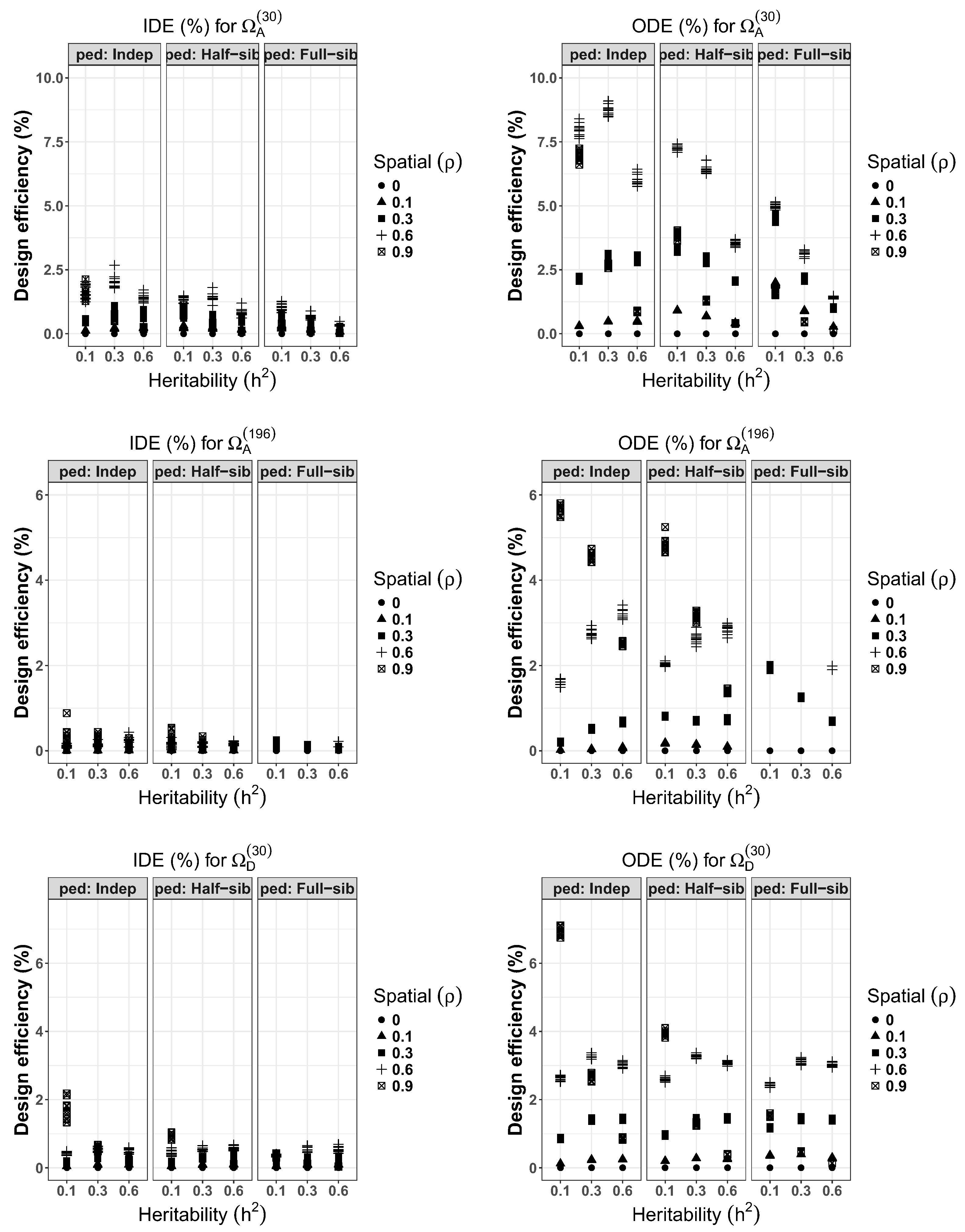
The evaluated conditions related to varying levels of heritability, genetic structure and spatial correlations for the RCB designs are shown in

Table 1. Summary statistics for Initial Design Efficiency (IDE%) and Overall Design Efficiency (ODE%) for randomized complete block (RCB) designs with 30 genotypes generated using A-optimality criterion ${\mathrm{\Omega }}_A^{\left(30\right)}$ and D-optimality criterion ${\mathrm{\Omega }}_D^{\left(30\right)}$ and for 196 genotypes generated using A-optimality criterion ${\mathrm{\Omega }}_A^{\left(196\right)}$. All designs were evaluated with $\lambda =10$ replicates per condition and iterated $p=5000$ times to improve the experimental layouts. ODE mean values that are starred ($\star$) are the overall largest improvements per combination of pedigree and heritability conditions.

Condition			Design ${\mathbf{\Omega }}_{\mathit{A}}^{\left(30\right)}$				Design ${\mathbf{\Omega }}_{\mathit{A}}^{\left(196\right)}$				Design ${\mathbf{\Omega }}_{\mathit{D}}^{\left(30\right)}$
Pedigree	${\mathit{h}}^{\mathbf{2}}$	$\mathit{\rho }$	IDE%	S.E.	ODE%	S.E.	IDE%	S.E.	ODE%	S.E.	IDE%	S.E.	ODE%	S.E.
Indep	0.1	0.1	0.120	0.002	0.305	0.002	0.004	0.001	0.017	0.000	0.046	0.001	0.124	0.001
		0.3	0.490	0.015	2.159	0.020	0.017	0.002	0.203	0.005	0.171	0.006	0.845	0.007
		0.6	1.636	0.087	7.975	0.075	0.102	0.010	1.602	0.019	0.417	0.013	2.627	0.022
		0.9	1.566	0.078	6.948	0.062	0.382	0.062	5.664 ${}^{\star }$	0.032	1.695	0.092	6.910 ${}^{\star }$	0.039
	0.3	0.1	0.211	0.005	0.481	0.003	0.008	0.001	0.042	0.001	0.093	0.003	0.236	0.002
		0.3	0.792	0.038	3.038	0.016	0.046	0.008	0.507	0.007	0.320	0.007	1.418	0.012
		0.6	2.043	0.084	8.739 ${}^{\star }$	0.065	0.140	0.016	2.767	0.031	0.541	0.019	3.272	0.017
		0.9	0.638	0.026	2.670	0.018	0.270	0.035	4.559	0.032	0.586	0.022	2.672	0.026
	0.6	0.1	0.227	0.006	0.483	0.005	0.013	0.002	0.063	0.003	0.098	0.001	0.249	0.002
		0.3	0.795	0.036	2.978	0.029	0.072	0.008	0.683	0.009	0.322	0.014	1.434	0.011
		0.6	1.435	0.051	6.025	0.071	0.253	0.027	3.213	0.036	0.524	0.021	3.041	0.024
		0.9	0.203	0.009	0.864	0.008	0.170	0.026	2.515	0.014	0.206	0.009	0.868	0.008
Half-sib	0.1	0.1	0.243	0.011	0.908	0.003	0.024	0.003	0.174	0.003	0.051	0.002	0.202	0.002
		0.3	0.689	0.016	3.310	0.027	0.036	0.006	0.805	0.006	0.166	0.006	0.969	0.007
		0.6	1.335	0.037	7.262 ${}^{\star }$	0.031	0.148	0.026	2.015	0.014	0.433	0.024	2.601	0.021
		0.9	0.928	0.040	3.848	0.040	0.341	0.035	4.834 ${}^{\star }$	0.055	0.934	0.024	3.943 ${}^{\star }$	0.024
	0.3	0.1	0.218	0.006	0.686	0.003	0.016	0.002	0.144	0.002	0.092	0.003	0.283	0.001
		0.3	0.643	0.021	2.898	0.028	0.051	0.007	0.704	0.007	0.283	0.007	1.430	0.010
		0.6	1.427	0.056	6.409	0.048	0.138	0.016	2.646	0.041	0.549	0.019	3.277	0.016
		0.9	0.304	0.021	1.287	0.010	0.158	0.029	3.161	0.029	0.319	0.015	1.307	0.012
	0.6	0.1	0.168	0.005	0.416	0.004	0.010	0.001	0.094	0.002	0.101	0.003	0.265	0.003
		0.3	0.555	0.025	2.054	0.010	0.064	0.006	0.714	0.010	0.331	0.014	1.446	0.010
		0.6	0.841	0.050	3.530	0.031	0.159	0.013	2.846	0.033	0.573	0.018	3.081	0.017
		0.9	0.100	0.005	0.403	0.004	0.096	0.011	1.405	0.012	0.092	0.005	0.390	0.003
Full-sib	0.1	0.1	0.262	0.017	1.955	0.015	0.039	0.005	0.623	0.007	0.056	0.002	0.358	0.003
		0.3	0.675	0.019	4.485	0.039	0.115	0.018	1.944	0.015	0.190	0.011	1.173	0.007
		0.6	1.064	0.047	5.004 ${}^{\star }$	0.034	0.116	0.018	2.829	0.032	0.362	0.010	2.419	0.016
		0.9	0.345	0.011	1.566	0.014	0.204	0.031	3.040 ${}^{\star }$	0.033	0.371	0.013	1.529	0.010
	0.3	0.1	0.166	0.007	0.899	0.004	0.023	0.003	0.467	0.003	0.091	0.004	0.398	0.001
		0.3	0.457	0.019	2.153	0.023	0.087	0.012	1.259	0.007	0.257	0.010	1.458	0.013
		0.6	0.671	0.031	3.128	0.031	0.126	0.014	2.245	0.010	0.540	0.026	3.114 ${}^{\star }$	0.023
		0.9	0.108	0.005	0.465	0.005	0.103	0.013	1.483	0.012	0.113	0.005	0.458	0.005
	0.6	0.1	0.087	0.003	0.271	0.002	0.014	0.002	0.204	0.001	0.094	0.002	0.284	0.004
		0.3	0.256	0.006	1.016	0.011	0.057	0.010	0.698	0.005	0.307	0.012	1.418	0.010
		0.6	0.346	0.017	1.421	0.013	0.145	0.023	1.896	0.014	0.553	0.026	3.029	0.018
		0.9	0.034	0.002	0.138	0.001	0.036	0.005	0.512	0.004	0.032	0.002	0.138	0.002

and Figure 1. The results presented here show the percentage improvement in terms of reduction in average variance of the treatment effects when A-optimality criterion is used and in terms of reduction in volume of the hypersphere when the D-optimality criterion based on the IDE% and ODE% design efficiency measures.

As, expected, the average IDE% values for RCB designs were all smaller than their respective ODE% values. This would confirm the fact that randomly generating hundreds of experimental designs and simply choosing the best with respect to A- or D-optimality criteria results in designs with lower efficiencies compared to optimized designs. After applying the optimization procedure to improve the experimental layout, the average highest ODE% of 8.739 (S.E. = 0.065) from the optimal designs under ${\mathrm{\Omega }}_A^{\left(30\right)}$ was obtained from the set of genetically unrelated individuals when $h^2=0.3$ and $\rho =0.6$. The only exceptions are the conditions with $\rho =0$ (i.e., no spatial correlation) that resulted in consistently null improvements. Relatively lower gains were observed within half-sib and full-sib families compared to structures with independent individuals. Specifically, the highest ODE% of 7.262 (0.031) among half-sib families occurred when $h^2=0.1$ and $\rho =0.6$ which was also the case among full-sib families that recorded the highest ODE% of 5.004 (0.034) when $h^2=0.1$ and $\rho =0.6$. Also experiments with either half-sib or full-sib families appear to achieve higher reduction of average variance of treatment effects when the heritabilities are very low (i.e., $h^2=0.1$). In addition, for any given heritability level, often highest design improvement was achieved when the spatial correlation level was 0.6.

The results from the larger experimental ${\mathrm{\Omega }}_A^{\left(196\right)}$ show that, on average, the overall highest ODE% was obtained when the experiments consisted of genetically unrelated individuals with $h^2=0.1$ and $\rho =0.9$ (ODE% = 5.664, S.E. = 0.032). Also, among the genetically unrelated individuals, when $h^2=0.3$, large improvements occurred when $\rho =0.9$ yielding a ODE% of 4.559 (0.032). However, for $h^2=0.6$, large design improvements (ODE% = 3.213, S.E. = 0.036) occurred when $\rho =0.6$. Considering the half-sib families, overall highest reduction in average variance of treatment effects of 4.834 (0.055) was observed when $h^2=0.1$ and $\rho =0.9$. Similarly, among the full-sib families, highest ODE% of 3.040 (0.033) was obtained when $h^2=0.1$ and $\rho =0.9$. These results indicate that an experiment with strong spatial correlations and with very low heritabilities may have considerable design improvements over experiments with high heritabilities and low spatial correlations.

The small experiments ${\mathrm{\Omega }}_D^{\left(30\right)}$ had the highest reduction in volume of the hypersphere (ODE% = 6.910, S.E. = 0.039) obtained when $h^2=0.1$ and $\rho =0.9$ among the genetically unrelated individuals. Similarly, the highest ODE% among half-sib family was 3.943 (0.024) obtained when $h^2=0.1$ and $\rho =0.9$. Experiments with full-sib families recorded highest design efficiencies of 3.114 (0.023) when $h^2=0.3$ and $\rho =0.6$. In general, for the same conditions ODE% values from D-optimality resulted in lower gains compared to A-optimality reflecting the nature of these optimization criteria. However, a Pearson’s product-moment correlation of $\sim 0.98$ between these criteria for ${\mathrm{\Omega }}_A^{\left(30\right)}$ and ${\mathrm{\Omega }}_D^{\left(30\right)}$ was obtained.

The number of successful swaps from the p = 5000 iterations for each condition and scenario were also monitored. The mean number of successful swaps for independent, half-sib and full-sib families in the ${\mathrm{\Omega }}_A^{\left(30\right)}$ scenario across all conditions were: 139 (range 96–208), 150 (93–244) and 178 (97–283). respectively. The average successful swaps under ${\mathrm{\Omega }}_D^{\left(30\right)}$ scenario were 185 (144–234), 190 (147–257) and 199 (131–260) for independent, half-sib and full-sib families, respectively. In contrast, under ${\mathrm{\Omega }}_A^{\left(196\right)}$ the successful swaps for the same genetic structures were larger, with values of 894 (830–959), 950 (828–1144) and 1024 (844–1281), respectively. In general, it was noted that higher number of successful swaps were obtained when the treatments had lower heritabilities and spatial correlation values.

3.2. Design Efficiencies for IB, AB and UR

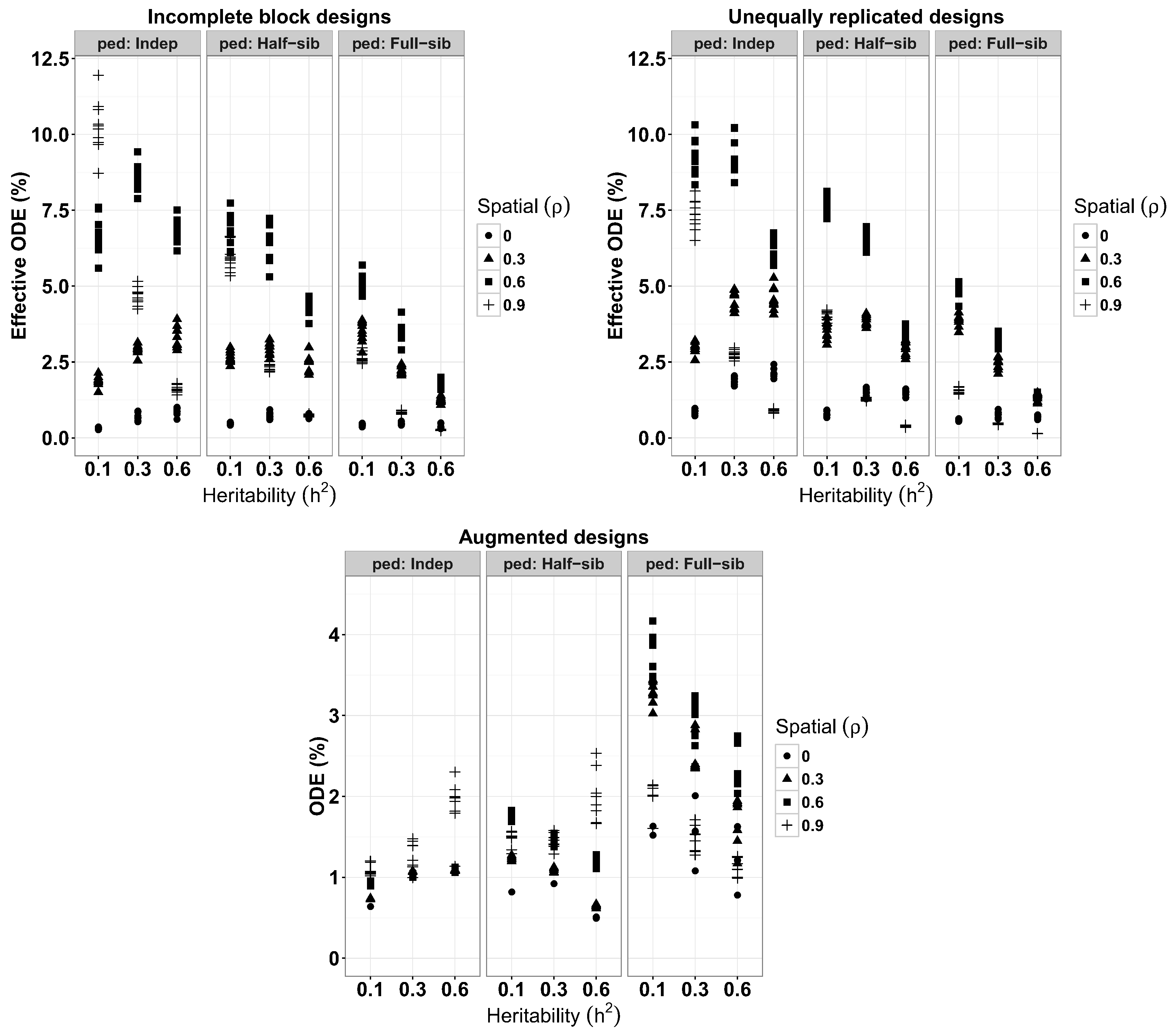
A summary of average ODE% for IB, AB and UR designs from each of the evaluated experimental conditions are given in

Table 2. Summary of average ODE% and their standard errors (S.E) for incomplete block (IB), unequally replicated (UR) and augmented block (AB) designs with varying genetic relatedness, spatial correlations ($\rho$) and narrow-sense heritability ($h^2$) based on $m=100$ initial designs, $\lambda =10$ replicates per condition and $p=5000$ iterations.

Condition		Indep		Half-Sib		Full-Sib
${\mathit{h}}^{\mathbf{2}}$	$\mathit{\rho }$	ODE%	S.E.	ODE%	S.E.	ODE%	S.E.
IB designs
0.1	0.0	0.317	0.009	0.468	0.011	0.421	0.012
	0.3	1.870	0.052	2.657	0.060	3.481	0.106
	0.6	6.663	0.193	6.824	0.163	5.082	0.089
	0.9	10.250	0.274	5.919	0.138	2.641	0.053
0.3	0.0	0.711	0.038	0.733	0.032	0.476	0.014
	0.3	2.902	0.050	2.950	0.063	2.220	0.041
	0.6	8.543	0.139	6.413	0.180	3.511	0.098
	0.9	4.672	0.090	2.313	0.038	0.858	0.016
0.6	0.0	0.872	0.039	0.709	0.017	0.371	0.020
	0.3	3.332	0.105	2.470	0.084	1.243	0.026
	0.6	6.854	0.122	4.337	0.087	1.833	0.047
	0.9	1.604	0.036	0.743	0.010	0.257	0.005
AB designs
0.1	0.0	0.639	0.000	0.820	0.000	1.589	0.020
	0.3	0.733	0.001	1.235	0.009	3.274	0.049
	0.6	0.922	0.006	1.765	0.018	3.752	0.093
	0.9	1.090	0.028	1.477	0.037	2.002	0.061
0.3	0.0	1.070	0.000	0.922	0.000	1.740	0.101
	0.3	1.074	0.002	1.095	0.009	2.546	0.088
	0.6	1.025	0.005	1.433	0.015	2.939	0.092
	0.9	1.275	0.062	1.446	0.034	1.474	0.056
0.6	0.0	1.113	0.000	0.506	0.002	1.333	0.090
	0.3	1.086	0.002	0.646	0.006	1.718	0.101
	0.6	1.092	0.006	1.191	0.018	2.387	0.083
	0.9	1.881	0.120	2.002	0.111	1.106	0.039
UR designs
0.1	0.0	0.889	0.025	0.787	0.028	0.584	0.010
	0.3	2.968	0.057	3.533	0.087	3.846	0.056
	0.6	9.283	0.184	7.650	0.085	4.914	0.075
	0.9	7.362	0.152	3.985	0.053	1.569	0.028
0.3	0.0	1.918	0.039	1.488	0.037	0.777	0.028
	0.3	4.566	0.092	3.870	0.056	2.438	0.056
	0.6	9.348	0.190	6.607	0.085	3.246	0.063
	0.9	2.747	0.043	1.290	0.014	0.472	0.006
0.6	0.0	2.131	0.042	1.474	0.030	0.699	0.016
	0.3	4.562	0.115	2.920	0.070	1.367	0.038
	0.6	6.207	0.110	3.417	0.070	1.389	0.022
	0.9	0.879	0.017	0.390	0.007	0.138	0.001

and Figure 2. IB designs achieved a highest average ODE% of 10.250 (S.E. = 0.274) when $h^2=0.1$ and $\rho =0.9$. For designs with $h^2$ of 0.3 and 0.6, mean highest reduction in average variance of treatment effects, with ODE% of 8.543 (0.139) and 6.854 (0.122), respectively, were obtained at $\rho =0.6$. For a given spatial correlation level, individual ODE% among full-sib families decrease with increasing heritability as shown in Figure 2 with average highest ODE% obtained when the spatial correlation was 0.6 (Table 2). Among half-sib families, a highest ODE% of 6.824 (0.163) was obtained when $h^2=0.1$ at $\rho =0.6$. For heritabilities of 0.3 and 0.6, mean highest ODE% of 6.413 (0.180) and 4.337 (0.087) were obtained when $\rho =0.6$, respectively. Improvements for IB designs with full-sib families were ODE% of 5.082 (0.089), 3.511 (0.098) and 1.833 (0.047) for $h^2=0.1$, $0.3$ and $0.6$, respectively, all of them obtained when $\rho =0.6$.

Results from the AB designs achieved the highest reduction of average variance of treatment effects among full-sib families when $h^2=0.1$ and $\rho =0.6$, yielding an ODE% of 3.752 (0.093). Among the full-sib families, designs with heritabilities of 0.3 and 0.6 obtained their highest ODE% of 2.939 (0.092) and 2.387 (0.083) at spatial correlations of 0.6. As with the IB designs, the ODE% increased with increasing spatial correlation from $\rho =0.0$ to $0.6$, and then decreased at a spatial correlation of 0.9 (see Table 2). For generated AB designs with genetically unrelated individuals, a trend was observed of highest design improvements achieved when $\rho =0.9$ at any levels of heritabilities with the highest value ODE% of 1.881 (0.120) obtained when $h^2=0.6$ and $\rho =0.9$. Similarly, an ODE% of 2.002 (0.111) was the highest improvement achieved among half-sib families when $h^2=0.6$ and $\rho =0.9$. Figure 2 shows individual ODE% values with a tendency to increase with larger heritability and spatial correlation among genetically unrelated individuals, and it decreased with increasing heritability among half-sib and full-sib families, except when $h^2=0.6$ and $\rho =0.9$ among half-sib families.

Unequally replicated designs yielded, a highest average improvement level of 9.348 (0.190) achieved when $h^2=0.3$ and $\rho =0.6$ observed among genetically unrelated individuals. At $h^2=0.1$, the highest average design improvement of 9.283 (0.184) was observed at a spatial correlation of 0.6. In addition, when $h^2=0.6$, the highest average ODE% of 6.207 (0.110) was obtained at $\rho =0.6$ among the genetically unrelated individuals. For a given heritability, among all genetic structures, ODE% increase with increasing spatial correlations up to $\rho =0.6$ and then dropped as spatial correlation increases to $0.9$. In general, for a specified heritability and spatial correlation level, ODE% values appear to decrease as genetic relationships increases (see Table 2). Also, for any given heritability, lower ODE% values were observed when spatial correlations were null ($\rho =0.0$) and in some conditions, when $\rho =0.9$ with $h^2=0.6$.

3.3. Analysis of Simulated Data for RCB Designs

A summary of the results obtained from the analysis of simulated data are presented in

Table 3. Summary statistics presented with Pearson’s correlation coefficient ($r_g$) and estimated heritabilities (${\widehat{h}}^2$) together with their coefficient of variation (C.V. %) for ${\mathrm{\Omega }}_A^{\left(30\right)}$ and ${\mathrm{\Omega }}_D^{\left(30\right)}$ scenarios. Each condition had $\lambda =50$ replicates each iterated $p=5000$ times. In Model 1, residuals were assumed to be uncorrelated and in Model 2, an $AR1\otimes AR1$ spatial correlation structure was fitted.

			Estimates under ${\mathbf{\Omega }}_{\mathit{A}}^{\left(30\right)}$						Estimates under ${\mathbf{\Omega }}_{\mathit{D}}^{\left(30\right)}$
Conditions			Half-Sib Family			Full-Sib Family			Half-Sib Family			Full-Sib Family
$\mathit{\rho }$	${\mathit{h}}^{\mathbf{2}}$	Design	${\widehat{\mathit{h}}}^{\mathbf{2}}$	C.V. %	${\mathit{r}}_{\mathit{g}}$	${\widehat{\mathit{h}}}^{\mathbf{2}}$	C.V. %	${\mathit{r}}_{\mathit{g}}$	${\widehat{\mathit{h}}}^{\mathbf{2}}$	C.V. %	${\mathit{r}}_{\mathit{g}}$	${\widehat{\mathit{h}}}^{\mathbf{2}}$	C.V. %	${\mathit{r}}_{\mathit{g}}$
Model 1
0.3	0.1	Initial	0.091	56.932	0.626	0.105	57.551	0.647	0.107	59.429	0.638	0.122	56.807	0.675
		Improved	0.107	57.958	0.625	0.107	67.372	0.660	0.130	49.984	0.666	0.129	61.648	0.682
	0.3	Initial	0.303	25.573	0.845	0.288	29.828	0.830	0.309	31.097	0.851	0.307	31.874	0.833
		Improved	0.302	30.783	0.854	0.311	29.985	0.827	0.315	26.223	0.85	0.301	32.012	0.839
	0.6	Initial	0.609	10.661	0.946	0.592	14.29	0.939	0.581	13.029	0.942	0.578	14.226	0.932
		Improved	0.594	11.505	0.943	0.574	14.425	0.932	0.582	15.934	0.941	0.574	18.943	0.923
0.6	0.1	Initial	0.119	48.321	0.644	0.117	61.060	0.618	0.126	46.390	0.659	0.114	61.020	0.682
		Improved	0.157	49.696	0.643	0.142	49.682	0.648	0.126	54.187	0.604	0.142	52.276	0.615
	0.3	Initial	0.291	30.602	0.852	0.317	26.024	0.844	0.315	26.474	0.859	0.308	32.348	0.832
		Improved	0.341	25.837	0.844	0.317	30.52	0.809	0.361	25.528	0.847	0.326	28.804	0.826
	0.6	Initial	0.602	12.046	0.950	0.613	11.383	0.940	0.601	13.728	0.945	0.608	15.518	0.939
		Improved	0.614	12.716	0.943	0.615	13.101	0.935	0.618	10.361	0.940	0.632	12.177	0.937
Model 2
0.3	0.1	Initial	0.088	55.335	0.685	0.100	58.724	0.665	0.088	61.306	0.686	0.106	56.899	0.694
		Improved	0.092	60.271	0.670	0.094	61.836	0.694	0.111	49.259	0.716	0.099	56.763	0.707
	0.3	Initial	0.284	25.788	0.874	0.282	29.295	0.857	0.307	27.117	0.876	0.302	29.865	0.857
		Improved	0.293	32.026	0.886	0.295	27.45	0.859	0.299	23.427	0.883	0.296	29.435	0.873
	0.6	Initial	0.594	12.037	0.954	0.582	14.984	0.949	0.577	11.451	0.955	0.560	14.180	0.944
		Improved	0.585	11.628	0.957	0.562	14.391	0.949	0.569	15.535	0.957	0.557	19.756	0.943
0.6	0.1	Initial	0.091	38.893	0.830	0.087	51.023	0.797	0.095	35.528	0.824	0.088	45.976	0.802
		Improved	0.099	35.675	0.858	0.088	37.522	0.828	0.090	36.586	0.844	0.084	36.736	0.832
	0.3	Initial	0.268	22.697	0.943	0.284	23.124	0.938	0.278	22.175	0.944	0.267	25.216	0.933
		Improved	0.292	21.367	0.951	0.275	20.051	0.937	0.295	20.827	0.953	0.282	23.933	0.940
	0.6	Initial	0.565	13.205	0.982	0.571	10.841	0.979	0.565	13.732	0.981	0.569	15.987	0.977
		Improved	0.571	13.579	0.984	0.571	12.637	0.981	0.560	17.916	0.983	0.576	13.523	0.982

and

Table 4. Summary statistics based on Model 2 with Pearson’s correlation coefficient ($r_g$) and estimated heritabilties (${\widehat{h}}^2$) together with their coefficient of variation (C.V. %) for ${\mathrm{\Omega }}_A^{\left(196\right)}$ scenario. Each condition had $\lambda =50$ replicates each iterated $p=5000$ times. Residuals errors were modeled using $AR1\otimes AR1$ spatial structure.

Conditions			Half-Sib Family			Full-Sib Family
$\mathit{\rho }$	${\mathit{h}}^{\mathbf{2}}$	Design	${\widehat{\mathit{h}}}^{\mathbf{2}}$	C.V. %	${\mathit{r}}_{\mathit{g}}$	${\widehat{\mathit{h}}}^{\mathbf{2}}$	C.V. %	${\mathit{r}}_{\mathit{g}}$
0.3	0.1	Initial	0.100	14.279	0.855	0.102	15.152	0.839
		Improved	0.102	14.390	0.860	0.101	13.428	0.837
	0.3	Initial	0.301	8.125	0.948	0.295	9.237	0.946
		Improved	0.303	8.011	0.950	0.306	7.070	0.949
	0.6	Initial	0.593	4.172	0.983	0.601	4.727	0.984
		Improved	0.595	4.851	0.983	0.593	3.956	0.983
0.6	0.1	Initial	0.109	14.169	0.900	0.107	11.142	0.893
		Improved	0.108	11.813	0.902	0.106	13.072	0.895
	0.3	Initial	0.321	6.999	0.967	0.319	7.669	0.969
		Improved	0.314	7.649	0.969	0.311	7.458	0.969
	0.6	Initial	0.616	4.784	0.990	0.614	3.416	0.990
		Improved	0.613	3.746	0.990	0.609	4.206	0.990

based on initial (i.e., un-improved) and final (i.e., improved) designs. These contain prediction accuracies for the estimation of genetic effects and heritabilities by fitting a LMM for the RCB design with and without a 2-dimensional separable spatial correlation structure denoted by Model 2 and 1, respectively.

Considering results from the improved designs and for ${\mathrm{\Omega }}_A^{\left(30\right)}$ scenario under Model 2 (Equation (3)), prediction accuracies of genetic effects among half-sib and full-sib families were found to be very high with $r_g=0.984$ and 0.981, respectively, obtained when $h^2=\rho =0.6$. Similarly, ${\mathrm{\Omega }}_D^{\left(30\right)}$ scenario under Model 2 resulted in strong prediction accuracies of genetic effects among half-sib and full-sib families with $r_g=0.983$ and 0.982, respectively, also obtained when $h^2=\rho =0.6$. In all cases, Pearson’s correlation coefficients from the no-spatial model (Model 1) were lower than those from Model 2 but still very strong. For instance, prediction accuracies for ${\mathrm{\Omega }}_A^{\left(30\right)}$ based on Models 1 and 2 among half-sib families were $r_g=0.943$ and $r_g=0.984$, respectively, obtained when $\rho =h^2=0.6$. As expected, the lowest predictive ability under each scenario was found when layouts had the lowest spatial and heritability values.

Results from ${\mathrm{\Omega }}_A^{\left(196\right)}$ scenario (Table 4) had much stronger predictive ability of $r_g=0.990$ for both half-sib and full-sib families when $h^2=\rho =0.6$. The lowest prediction accuracy occurred when $h^2=0.1$ and $\rho =0.3$ resulting in $r_g$ values of 0.860 and 0.837 for half-sib and full-sib families, respectively. As expected, for the three scenarios (${\mathrm{\Omega }}_A^{\left(30\right)}$, ${\mathrm{\Omega }}_A^{\left(196\right)}$ and ${\mathrm{\Omega }}_D^{\left(30\right)}$), for a given level of spatial correlation, $r_g$ increased with increasing $h^2$ and similarly, for a given $h^2$ value $r_g$ increased with $\rho$.

Precision of the estimated heritabilities, measured using coefficient of variation (C.V. %), was found to be largest for smallest $h^2$ values, decreasing with increasing $h^2$ in both half-sib and full-sib families. In addition, C.V. % of heritability decreased considerably with increasing $\rho$ values. Conditions with smaller heritability values were relatively more variable, presenting higher C.V. % than for those with larger heritability. For a given heritability value, prediction accuracies increased with increase in spatial correlations only for the spatial correlation model (i.e., Model 2). The C.V. % of heritability for ${\mathrm{\Omega }}_A^{\left(196\right)}$ were notably smaller than for ${\mathrm{\Omega }}_A^{\left(30\right)}$ and ${\mathrm{\Omega }}_D^{\left(30\right)}$ scenarios, a result likely due to the larger number of experimental units used.

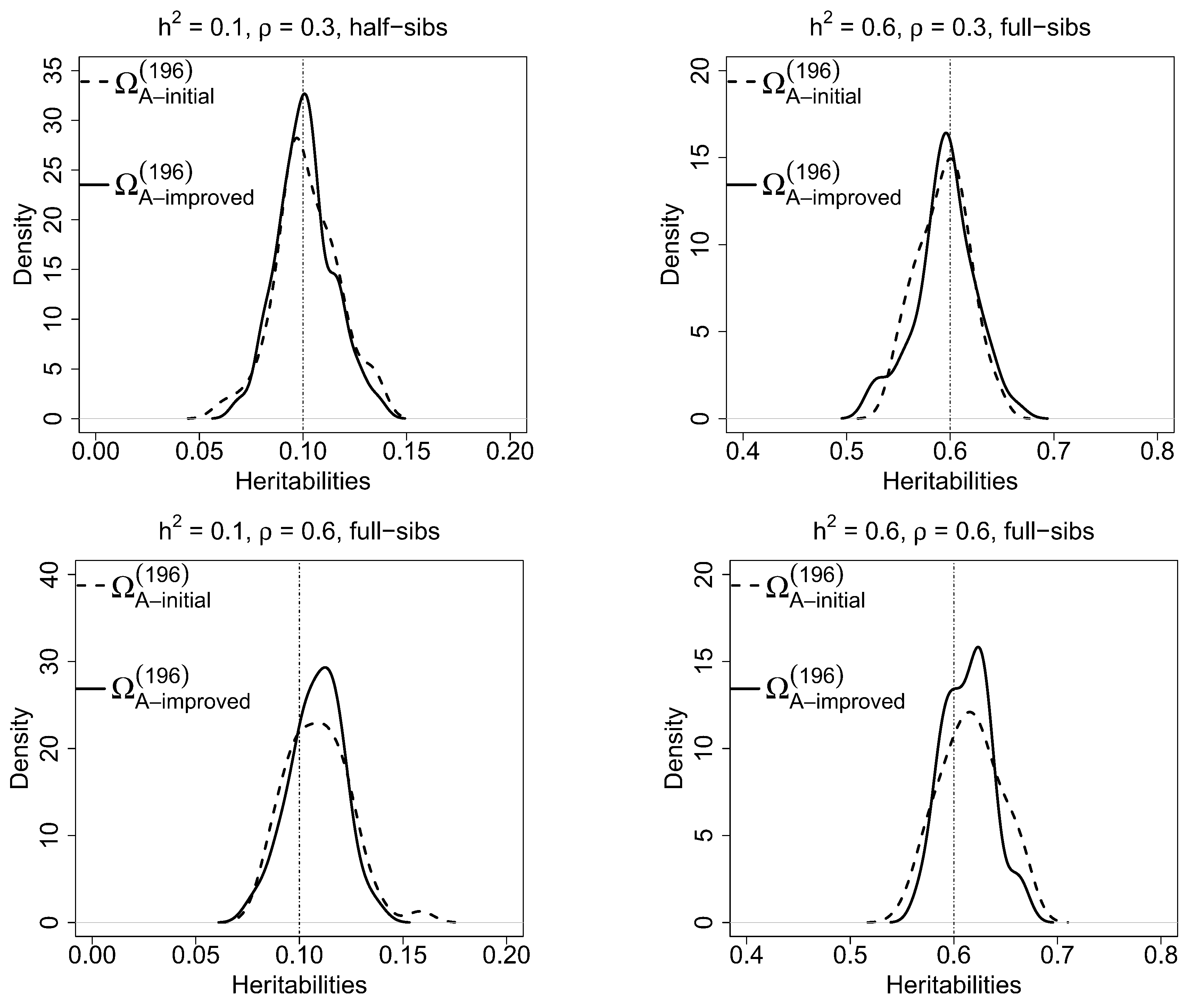
Kernel densities of estimated heritabilities for Model 2 based on ${\mathrm{\Omega }}_A^{\left(196\right)}$ scenario are shown in Figure 3 for selected conditions. Here, comparisons of estimated heritabilities between the initial and improved designs for full-sib and half-sib families are presented, which clearly indicates that final designs provide greater precisions (i.e., narrower distributions) than initial designs in estimating heritabilities.

4. Discussion

The primary aim for this study was to focus on algorithms and statistical procedures that can be useful on the generation of optimal field designs with correlated observations and to assess their efficiency considering a wide spectrum of typical field conditions. Although we demonstrate how to simulate data from a RCB design in Section 2.5, this was only secondary to the generation of optimal designs and was necessary to show how we simulated the data for analysis and evaluate the accuracy and precision of genetic effects and heritabilties that were analyzed using ASReml-R v. 3.0 [13]. Further details on simulating data for other complex designs have been discussed by other studies [5].

Different experimental designs, and varying environmental and genetic conditions have a strong influence on the efficiency of field experiments. In this study, it was shown that, by the use of a linear mixed model framework to account for genetic relatedness and spatial correlation, it is possible to achieve important efficiency gains for the generation of experimental designs. Unlike other studies that have discussed optimality procedures by fitting mainly fixed effects models (e.g., [20,23]), the implemented procedure reported here provides with results that are practical for an array of field trial scenarios commonly used in plant studies.

For RCB designs, under the absence of spatial correlations (i.e., $\rho =0.0$), regardless of the level of heritability and genetic structures, there are no gains in optimizing designs using the implemented swap algorithm. In contrast, for IB, UR and AB designs, there were some moderate gains achieved for the evaluated conditions. This is expected due to the balanced and orthogonal nature of the RCB designs, whereas for the other designs rearrangement of the experimental units (for example, between different incomplete blocks), yields to better treatment pairwise comparisons. However, zero spatial correlation might not be a reasonable assumption, as in practice for any field trial there is always some level of spatial correlations. Nevertheless, under non-zero spatial correlations, all scenarios showed considerable improvements, particularly for the independent genetic structure. However, the positive effect of strong spatial correlations tends to diminish as the level of genetic relatedness between the treatments increases.

The input required for the generation of an improved experimental design under the proposed pairwise swap algorithm, includes a choice of number of iterations and optimality criterion. Figure 4 presents an illustration for a RCB design based on $h^2=0.3$ and $\rho =0.6$ for genetically unrelated individuals, half-sib and full-sib families for ${\mathrm{\Omega }}_A^{\left(30\right)}$, ${\mathrm{\Omega }}_D^{\left(30\right)}$ and ${\mathrm{\Omega }}_A^{\left(196\right)}$ scenarios based on $p=$ 50,000 iterations. For small RCB designs (${\mathrm{\Omega }}_A^{\left(30\right)}$ and ${\mathrm{\Omega }}_D^{\left(30\right)}$), the rate of improvement was high until 5000 to 10,000 iterations and flattens out thereafter. The large RCB design (${\mathrm{\Omega }}_A^{\left(196\right)}$) showed that there was room for improvement even after 50,000 iterations, a result that is expected from experiments with large number of treatments [20]. Interestingly, there was a small number of successful swaps. For example, with ${\mathrm{\Omega }}_A^{\left(30\right)}$ scenario, for independent, half-sib and full-sib families, these reached only 178, 172 and 198 cases, with ODE% of 9.67, 7.00, and 3.52, respectively. In contrast for ${\mathrm{\Omega }}_A^{\left(196\right)}$, the successful swaps were 2589, 2685 and 2616, for the same genetic structures. Nevertheless, using 5000 iterations provides with a useful stopping criteria that limits the time required to run the optimizing procedure.

The decision between A- and D-optimality criteria depends on the aim, where the A-optimality criterion minimizes the average treatment effect variance and D-optimality criterion minimizes the generalized variance of the treatment effects, hence it considers covariances between pairs of treatment effects. Nevertheless, in this study, a strong Pearson’s product-moment correlation of $\approx 0.98$ between A- and D-optimality criteria was detected. This is not completely unexpected as both criteria are a convex function of the eigenvalues of the information matrix [22,23].

Several measures of design efficiency can be evaluated. In this study, overall design efficiency (ODE%) was used. Other measures have been proposed, such as the average efficiency factor (a.e.f.) [20] that compares the average pairwise variance of a given design layout against an RCB design with the same number of treatments and replicates. Nevertheless, a.e.f is only defined for designs where treatment is considered a fixed effect.

For all conditions evaluated the current study has shown that, for RCB designs based on A-optimality criterion, gains of up to 8.7% can be achieved. Both small and large experiments with half-sib and full-sib families can achieve greater improvements under low heritability levels and moderate spatial correlation. Filho and Gilmour [21] also reported larger improvements on those layouts with genetically unrelated individuals against those that accounted for genetic relatedness; however, their residuals were assumed independent.

For the data simulated for an RCB design, high prediction accuracies (≥0.90) of genetic additive effects were obtained from both initial and improved experimental layouts from models with and without spatial correlations. As expected, better prediction accuracies were found for the model that incorporated spatial correlations, particularly for the improved designs. This result is similar to the findings reported by [5]. The current study has found that estimation of heritabilities was more accurate under improved designs for both models. Also, as expected, genotype effects estimated under layouts with small heritability values will exhibit larger C.V. % compared to layouts with large heritability values, and when the spatial correlations are low, the C.V. % for estimated heritability is larger, and vice-versa. The prediction accuracies of genetic values from larger experiments is higher compared to that from small experiments, but similar trends are observed as the accuracy increases with increasing levels of heritabilities.

In the case of more complex designs, such as IB, AB and UR, the highest average variance reduction of treatment effects of about 8.54%, 1.03% and 9.35%, respectively, were achieved when conducted with genetically unrelated individuals with heritabilities of $0.1$ and spatial correlations of $0.6$. As indicated earlier, unlike RCB designs, it is still possible for these designs to improve their efficiencies even when spatial correlation is zero. It is expected that the improvement of the generation of these designs will require large number of iterations as a results of their unbalanced nature.

The proposed swap algorithm and procedures used here can be extended to include other experimental designs, genetic structures, and spatial variance-covariance structures (such as the ones described by [12,13,14,37,38]). In addition, instead of using pedigree information to calculate a numerator relationship matrix, molecular markers can be used to calculate a genomic relationship matrix [17]. The use of the relationship matrix within the mixed model framework is limited to only describing the additive genetic effects. However, the linear models can be extended with other matrices to consider all genetic effects, such as dominance and epistatis.

A similar algorithm to the one proposed here for the generation of experiments was developed by [4], which also deals with correlated effects and residuals using a different optimization approach. However, it is expected that these two algorithms may result in nearly identical optimal solutions, given the similarity of these methods. Nevertheless, in the present study, findings about generation of experiments under an array of varying conditions apply to any algorithm that generates an optimal design, and this should assist on the use of these tools.

In order to generate field experiments, there is a need for known values of the different variance components (e.g., spatial correlation). This could be a limitation of the proposed algorithm; however, for most mature breeding programs there is always some level of information about what to expect on a field experiments. For example, some fields are dominated by patches (i.e., high spatial correlations) others are dominated by gradient. In addition, usually the same farms are used repeatedly to establish breeding trials, and pedigree information often is available to be used to calculate relationship matrices that can be incorporated in a design to be generated. The present study has evaluated an array of varying typical field conditions that can be used; hence, it is possible to asses and select the most appropriate condition to generate a desired design. Finally, even if a generated design is not fully optimum for its field conditions, it is likely to be always better than a design that ignores any type of spatial and/or genetic correlations. More complex designs than RCB might be required when conducting experiments with large number of treatment levels as is common on breeding experiments. Thus, it is advisable in these cases to use more complex layouts such as IB designs.

This study has demonstrated how to generate experiments with random initial arrangements and optimize them considering both spatial and/or genetic relatedness. When designing complex field experiments, it is important to start with an optimal design. Generating an optimal experiment assuming all parameters are fixed with no sort of correlations has been implemented by many other studies such as CycDesigN [20]. A two step approach can be used where after the initial design is generated assuming no spatial or genetic correlations, then the second stage superimposes these realistic conditions. The strength of our method is that our algorithm can take any design and optimize it. The R-codes developed allow the user to input any initial design, or generate the design within our software. If the initial design is generated within this software, our current approach starts with a random design and models these correlations simultaneously in one step. The two-step approach was not implemented and can be viewed as a limitation of the study, but can be implemented in the future. For large experiments, long computation time were required to generate improved designs using a desktop computer. For example, the time taken for ${\mathrm{\Omega }}_A^{\left(30\right)}$ scenario for 5000 iterations, was ∼2 min and for ${\mathrm{\Omega }}_A^{\left(196\right)}$ scenario it took ∼30 min. Improved computation can be implemented with faster code and software to enable evaluation of experiments with large numbers of treatments. Additionally, other stochastic search algorithms, including simulated annealing, could yield potentially faster optimizations when compared to the pairwise swap algorithm proposed here.

5. Conclusions

This study has demonstrated that simultaneous considerations for genetic structure and spatial correlations can be incorporated to generate better experimental designs with important improvements in relative design efficiency and prediction accuracies of random treatment effects. Also, for RCB, IB, AB and UR designs higher relative design efficiencies are achievable from genetically unrelated individuals compared to experiments with half-sib and full-sib families. For RCB designs with half-sib or full-sib families, the optimization procedure may yield to important improvements under the presence of mild to strong spatial correlation levels and relatively low heritability values. As expected, accuracy of prediction of genetic values improves as levels of heritability and spatial correlations increases.

References