Article

May the Inclusion of a Legume Crop Change Weed Composition in Cereal Fields? Example of Sainfoin in Aragon (Spain)

1
Department of Plant Health, Centro de Investigación y Tecnología Agroalimentaria de Aragón, Instituto Agroalimentario de Aragón-IA2, CITA-Universidad de Zaragoza, 50059 Zaragoza, Spain
2
Departamento de Agricultura, Ganadería y Medio Ambiente, Diputación General de Aragón, 50071 Zaragoza, Spain
3
Departamento de Ciencias Agrarias y del Medio Natural, Instituto Agroalimentario de Aragón-IA2, CITA-Universidad de Zaragoza, 22027 Huesca, Spain
4
Dep. Hortofructicultura, Botànica i Jardineria, ETSEA, Agrotecnio, Universitat de Lleida, 25198 Lleida, Spain
*
Author to whom correspondence should be addressed.
Submission received: 21 January 2019 / Revised: 27 February 2019 / Accepted: 9 March 2019 / Published: 14 March 2019
(This article belongs to the Special Issue Weed Management in Annual and Perennial Cropping Systems)

Abstract

:
Onobrychis viciifolia (Scop.) (sainfoin) is promoted in the Spanish Aragón region through the Agro-Environmental Schemes (AES) since 2007 with the aim of enhancing biodiversity. Also, in other countries, the interest in this legume crop is growing due to its rusticity and beneficial effects on the soil and livestock. However, the effect of the crop on weed flora in the subsequent cereal crops has hardly been investigated yet. With this aim, weed flora has been characterised in 2011–2014 in sainfoin fields in the second and third year of establishment (S2 and S3), in cereal monocrop (CM), in cereal after sainfoin (CS) and in organic cereal fields (OC). Additionally, the soil seedbank was determined in two years in CM and S3 fields. Weed species richness of emerged flora and of the soil seedbank was highest for sainfoin and lowest for CM, being intermediate for OC and CS regardless of the sampling year. The most feared weed species in winter cereal did not increase by growing sainfoin or in CS compared to CM. Curiously, summer annuals dominated in the soil seedbank. Sainfoin fields cause thus a shift in the weed flora, which does not seem to damage subsequent cereal crops provided fields are mouldboard ploughed after sainfoin.

1. Introduction

Since the new Common Agrarian Policy enacted in 2015, so-called “greening” encourages farmers to include different crops in their rotation. In Spanish dryland areas, this measure has led to an increase in sowing legume crops in low-land areas, mainly vetch and lucerne. Between 2007 and 2014, one of the Agri-Environmental Schemes (AES) financed by the Aragón Government has been promoting sainfoin (Onobrychis viciifolia Scop.) with the objective of favouring steppe fauna, especially enhancing the nesting and reproduction of steppe birds. In the new Rural Development Plan (2015–2020) this measure has been included once more aiming to combine agriculture and environmental protection. Sainfoin is a forb belonging to the Fabaceae family and is grown as perennial forage on calcareous soils. The main climatic limitations of sainfoin are high temperatures and soil temperatures exceeding 10 °C causing a decrease in crown, taproot and fine root biomass [1]. On the contrary, sainfoin seedlings withstand temperatures below zero, demonstrating an adaptation to the last spring frosts, which occasionally occur in cold areas after sowing [2], being a well-adapted crop to the cool temperate zones of Europe [3]. This crop is also tolerant to drought and resistant to the most common pests and diseases [4,5] excepting, e.g., powdery mildew [6], winter crown rot caused by low-temperature fungi [7] or a beetle affecting sainfoin recently described in Turkey [8]. In addition, this crop does not respond well to inputs as nitrogen: applying more than 80 kg N ha−1 did not result in significant increase in the forage dry matter in none of four tested cultivars [9]. Due to all these characteristics, this species is an appropriate crop to grow on poor soils at cool temperatures and dry summers in areas with continental climate where other forage crops as lucerne fail due to lack of water or too low temperatures.
Sainfoin was first used as a crop in the sixteenth century in France and, due to the acceptable biomass productions on poor soils where other forage crops, such as lucerne, do not grow correctly, the Spanish Ministry of Agriculture promoted its use at the end of the 1960s. In 2015, this crop was grown on a total of 22,350 ha with Teruel province (in the Aragon region) producing the most (6947 ha) [10]. Traditionally, this region has produced the most sainfoin in Spain (12,392 ha), with the mean seeded surface in this province in years 1946–2000 corresponding to 31% of the total Spanish acreage devoted to this crop [11]. However, a massive reduction in the number of sheep livestock in the last decades has resulted in less sainfoin being planted.
The requirements for farmers in the Agri-Environmental Schemes (AES) financed by the Aragón Government are (a) growing sainfoin during 5 years in a surface of 2 to 50 ha, (b) removing the crop at latest 4 years after implantation and rotating at least one year with a different crop, (c) doing a single mowing between 1st of June and 30th August and (d) no grazing or mowing between 1st May and 1st of June to favour steppe bird nesting [12].
Following the results of a farmer survey conducted in 2014 in Aragon, 82% of them had grown this crop before the AES payments for more than 15 years, some even for 30 years [13]. Most of the farmers (70%) seed the crop in spring, with irregular sowing rates ranging between 50 and 150 kg ha−1, and only 23% of the farmers mow the crop during the first year provided there are specially good conditions in the first months for the crop development. The most common practice is the combination of mowing and pasturing (68% of the farmers) depending on the forage demand. Mowing is generally conducted between June and July (80% of the cases) which is compatible with the AES requirements. Sheep usually graze sainfoin in autumn–winter because the crop is green the natural pastures are generally dry. The plots are maintained for 2–5 years depending on the crop establishment and climatic conditions with 70% of the farmers growing sainfoin for 3 to 4 years. Only farmers sowing sainfoin in direct drill (14%) use herbicides in winter, the rest of the producers do not perform any weed control method other than mowing or allowing pasture. The crop is judged to be normally positive for the crop rotation (95% of the enquired producers), some farmers denoting general benefits in the following crops even two years after. Very probably, these benefits are a sum of different advantages besides the nitrogen fixation, such as favouring soil microorganism diversity and enriching soil activity, compared to fields managed in cereal monocrop.
The high content in tannins of sainfoin [14] offers multiple advantages for animals grazing the forage. For example, unlike other legumes such as alfalfa, sainfoin does not cause bloat in grazing animals [15]. In dairy cows, inclusion of sainfoin silage in fodder rations seems to reduce methane production per kilogram of dry matter intake and nutrient digestibility and moreover improves milk production [16]. Sainfoin has also anthelmintic effects in goats and sheep [17], and recent research also suggests reduction of the parasitic lamb coccidiosis [18]. All these advantages are causing an increasing interest in this crop in several countries for example in Canada [15], Austria, Switzerland [19], the UK [5] or even Russia (Siberia) [20], as well as in the areas where this crop has been traditionally grown, such as in Iran, Turkey and Spain.
Despite its rusticity, sainfoin is more difficult to maintain than other legumes [5,21] so that it is often sown in a mixture with either grasses or lucerne [8] despite in Aragón sainfoin is sown alone (or undersown in the previous winter cereal). The main advantage of the use of mixed crops is that weed infestations in mixtures are generally lower as compared to pure grown swards [22]. However, in these mixed crops sainfoin may also suffer from competition of grasses [23] so that these mixtures need to be selected carefully. Very little genetic improvement has been carried out in the last 60 years [4,5] despite the characterisation of many local accessions in different countries [24], thus there is a limited availability of well performing varieties [25]. It is generally accepted that sainfoin as well as other legumes should be more promoted in agriculture so that research generating new information around this crop is welcome.
In the study area where this crop is promoted, no technical improvements have been made in the last decades and little is known about the possible effect of including this crop in the cereal rotation from the weed infestation point of view. The effect of the different management options such as mowing, grazing and the combination of both on the weed species composition of sainfoin fields has been documented in the Eastern Pyrenees [26], but only preliminary data has been published from the Aragon region [27]. It is well-known that growing monocultures easily generates weed problems [28] but hardly any information is available on the possible influence on weed infestations by including sainfoin in the crop rotation being winter cereal the main crop. As no specific weed control is conducted in sainfoin fields it is necessary to demonstrate that this crop will not carry over weeds in the following winter cereal [13].
The objectives of this work are (1) to describe the weed flora in sainfoin fields in the second and third years (S2 and S3) in cereal monocrop fields (CM), in cereal grown after sainfoin (CS) and in organic cereal fields (OC) and (2) to evaluate the weed soil seedbank in S3 compared to CM and, thus, to find out if growing sainfoin during three years increases the abundance of weeds in following cereal crops.

2. Materials and Methods
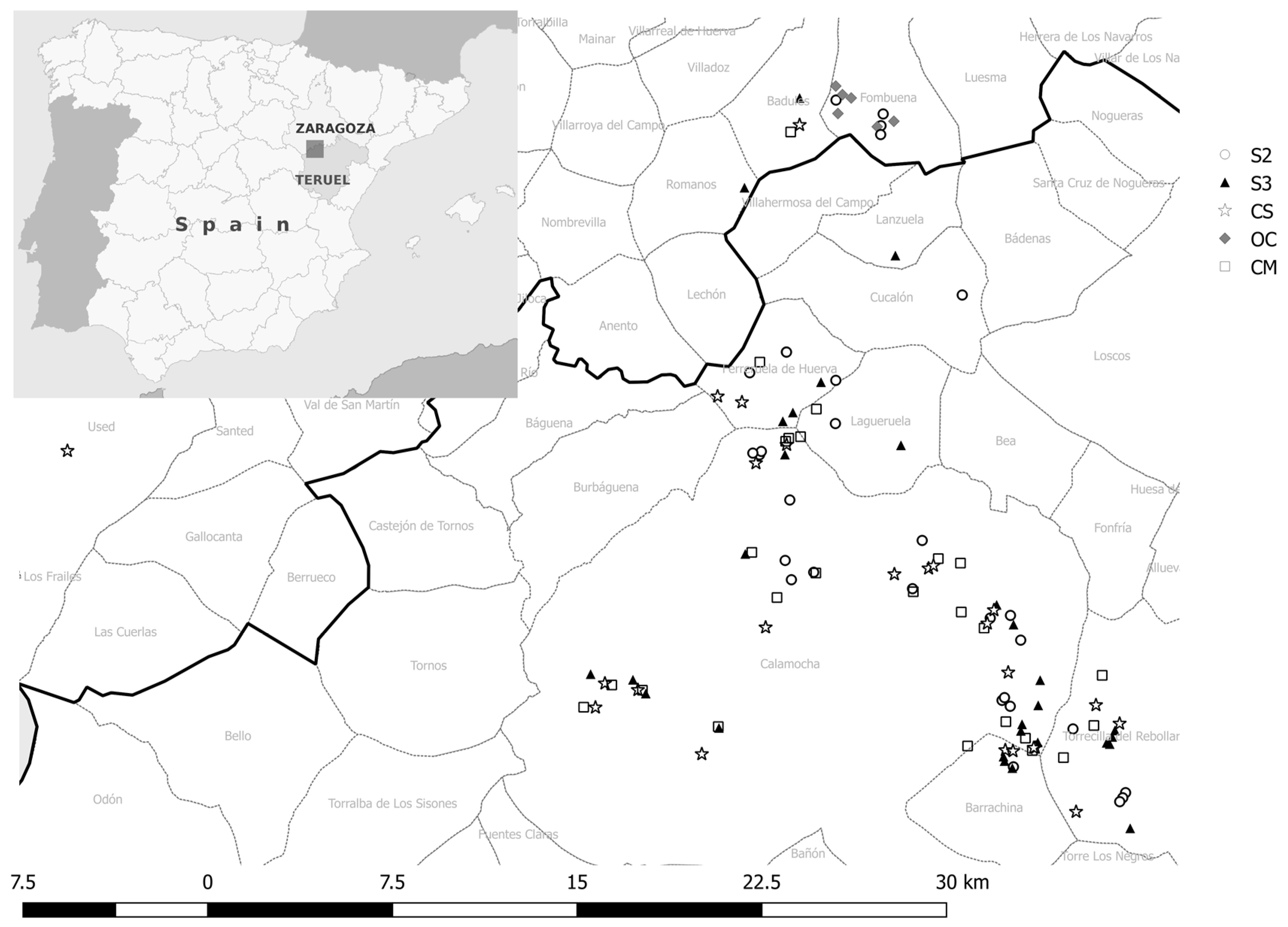
2.1. Field Surveys

Surveys were conducted during May 2011, 2012, 2013, and 2014 on cereal in the surroundings of Calamocha (Teruel, Aragon, Spain) where this crop is well-represented. Fields were chosen in several villages ranging from latitude 41°8′21.16″ N to 41°4′43.48″ N and longitude 0°52′50.71″ W and 0°43′50.90″ W. A total of 108 fields were sampled. Each year, a total of 24 fields of ~1 ha were selected (6 CM, 6 S2, 6 S3 and 6 CS fields), and selecting different plots each year to increase possible variability. Additionally, 6 OC fields were included in 2013 and other 6 plots in 2014 as near as possible to the other fields belonging to the only two organic farmers of the area, one north to Calamocha and the other 20 km south (Figure 1). Irrigated fields near the rivers were excluded to avoid introducing more factors. Due to the marginality of this crop, it was not easy to find the appropriate 24–30 fields each year of the needed surface and crop characteristics and these fields were often difficult to reach.
In the area, farmers occasionally spray postemergence herbicides in CM against broadleaved species and, in case of grass weed infestations, specific herbicides might be applied in pre-emergence or during the winter but herbicides are not used all years. Opposite, chemical fertilisers are commonly used, normally split in preplant dressing and a second top dress at tillering in spring. Contrary, OC is grown without herbicide use and fertilising only with organic materials. Mouldboard plough is generally used each year in conventional farming but not in organic farming where chisel and other noninversion tillage tools are used.
The survey was conducted in full sainfoin flowering before mowing (stages 65−71 in BBCH scale) [29] and in cereal earing (stages 59–73 in BBCH scale) to allow maximum species identification. Survey dates were 12th to 20th May in 2011, 16th to 25th May in 2012, 20th to 30th May in 2013 and 21st to 28th May in 2014. Three persons walked across the field in zigzag of the whole plot or covering approximately one hectare if the plot was bigger. Species appearing only in the field edges (first 2 m) were discarded as it is known that species richness is bigger in the boundaries [30]. While walking through the field they announced the presence of each new seen species and a fourth person noted down the name. When no new species were detected any more, an averaged abundance value, representative for the whole plot, was assigned to each identified weed species following the scale of Marnotte [16]. This method was considered the best to give a total picture of the weed infestation on the whole plot compared to counts in frames and allowed to describe the flora of many fields each year. The CEB scale (Comité d’Essais Biologiques) [31] relates plant density with weed soil cover, allowing a better estimation in the lower abundance categories and ranges from 1 to 9, which corresponds to categories of soil cover percentages of <1% (rare plants), 1–7% (<1 plant m−2), 7–15% (>1 plant m−2), 15–30%, 30–50%, 50–70%, 70–85%, 85–93% and 93–100%, and has been successfully used in other surveys [32].
Additionally, crop height and crop soil cover were evaluated in the field during the survey. In laboratory, complementary information data including the exact plot area, perimeter, plot slope and altitude of the fields were determined using the Spanish official Geographic Information System of Agricultural Plots (SigPac database, 3.2.) [33]. Fields in the area are generally quite small due to the orographic conditions and accomplished 1.5 ± 0.08 ha and only 15% of the selected fields measured less than 0.75 ha. Mean altitude of the sampled fields was 1067 ± 7.9 m within the range of 907 to 1243 m and 75% of the fields were located over 1000 m altitude.

2.2. Seed Bank Determination

In 2012 and 2013, soil samples were taken in 13 S3 and in 10 CM fields. For each field, six subsamples were extracted following a cross shape, excluding the boundaries as in the field survey. Stones and evident plant rests were eliminated and samples mixed together. Sampling depth was 7.5 cm, which meant an important sampling effort as soils were very stony, had not been ploughed in the last 3 years and, additionally, suffered compaction after sheep grazing. A total volume of approximately 1 L of soil was sampled per field. The soil in the cereal fields was obviously less compacted. Soil was kept in plastic bags at 4 °C until processing. Samples were divided in half and two 0.5 L cylinders made with a 0.6 mm mesh were filled with each sample, excessive soil was discarded. Soil was washed using an own-made elutriator by the Weed and Plant Ecology Group of the Lleida University. The extractable method was preferred to the germinable one because of the higher amount of seeds extracted with the first one [34]. After one and a half hours of washing, rests were collected and small stones were later eliminated progressively with manual sievings. Seeds with similar aspects were grouped and photographed through binoculars (Olympus SZX7, Tokio, Japan, of 0.8–5.6 magnification using the camera Optika 4083.12LT, Ponteranica, Italy), and were counted and identified using appropriate literature [35,36,37].

2.3. Weed Species Composition: Most Frequent and Most Abundant Weeds, Richness, Cover, Shannon Index and Multivariate Analysis
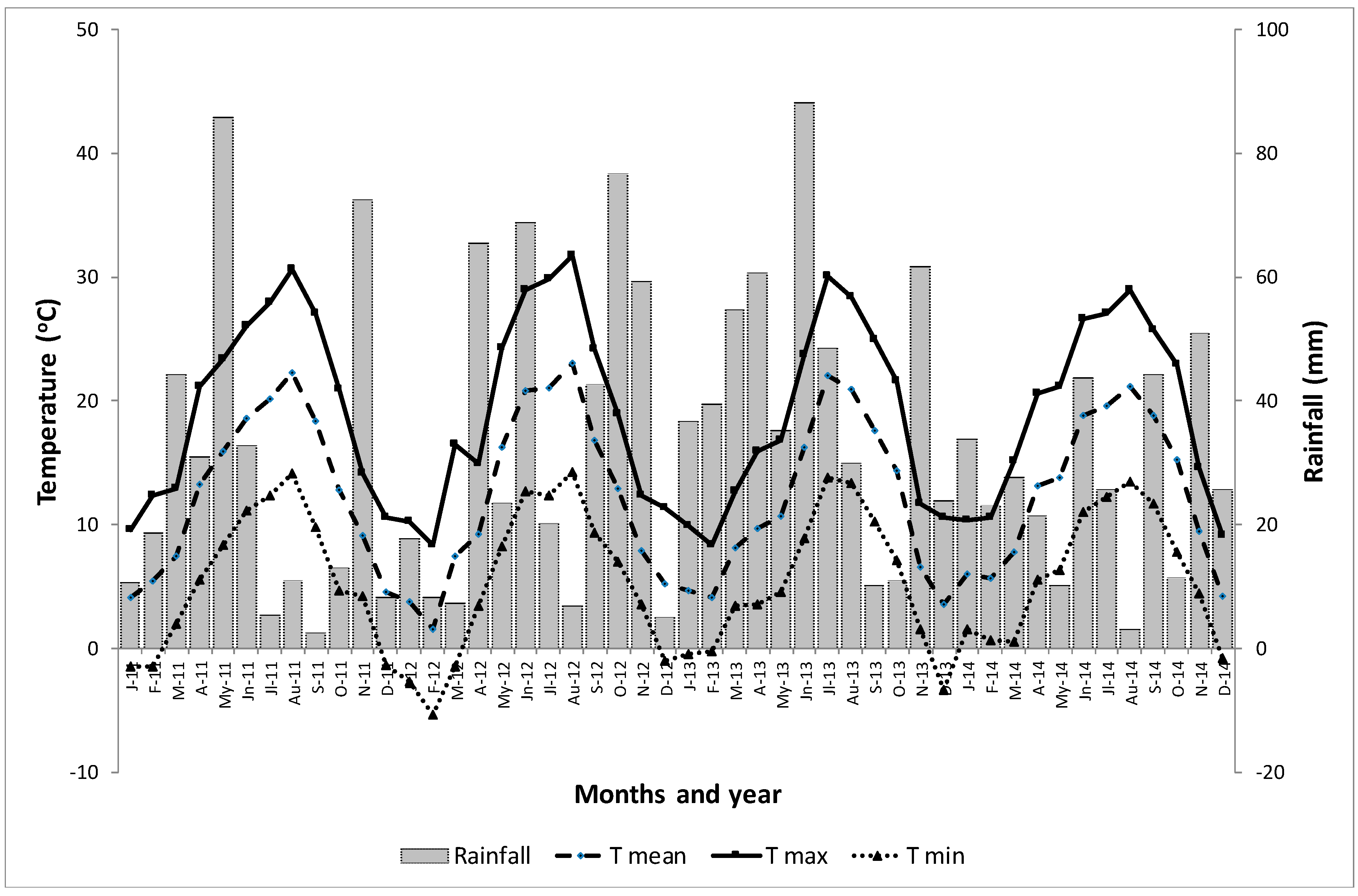
To identify the most damaging weed species in each crop, abundance weed data from the four sampling years were pooled together for each crop separately to calculate frequency and mean average when found. Those species with soil cover ≥3%, when present, and those with frequency ≥30%, were selected. Weed frequency was calculated as a percentage of fields where each species was present for each crop separately but for all years together. These limits were chosen taking into account the threshold recommended by the Spanish Ministry of Agriculture in the Integrated Pest Management guide for cereals [38]. No official guidelines are published for forage crops yet, but following [39] private companies classify lucerne into the following quality classes depending on the visual weed content of the forage: supreme quality: 0% weeds; premium quality: up to 3% weeds; first class quality: 3–8% weeds; second quality: 8–25% weeds; and ordinary or third quality: more than 25% weeds. Thus, the 3% limit was considered also an appropriate limit for sainfoin. Thus, weed species exceeding both parameters of frequency and abundance are considered to be the most threatening for farmers.
Shannon diversity indexes applied to weed abundance were calculated for the weeds found at each field and for the seeds found in the soil following [40].
H = i = 1 s p i   ln   p i   where   p i = n i N
where S is species richness in each sample, pi = Ni/N, Ni is abundance or the number of seeds of species i and N is the total abundance or seed number of each sample. Species and seed richness data was tested for normality and homoscedasticity, seed richness needed   x transformation and standard ANOVA and Student–Newman–Keuls mean separation tests were performed on these data using SAS 9.4. (Cary, NC, USA) [41]. Weed cover, crop cover and crop height data could not be normalised and data was analysed using the nonparametric one-way ANOVA test of Kruskal–Wallis using the R Project for Statistical Computing [42]. Additionally, the nonparametric two-sample Wilcoxon rank-sum test was used to contrast paired samples on two different crops.
Due to the nonsignificant interaction of “year x crop”, frequency and abundance data of all four years was pooled together for each crop to detect the most frequent and most abundant species.
Data was checked for normality and homoscedasticity and submitted to ANOVA. As the factor “year” was not significant, data was pooled together and analysed with a Student–Newman–Keuls separation test using SAS v. 9.4. [41].
A Canonical Correspondence Analysis (CCA) was performed using Canoco 5 (Ceske Budejovice, Czech Republic) [43]. Tested variables were crop, year, plot slope, altitude, crop height, crop soil cover, field perimeter/area and weed soil cover. Variables were selected stepwise using the Monte Carlo permutation test with 999 permutations.
Species assemblages were analysed using the mean abundances of plant species per field. A matrix of similarities was obtained with Bray–Curtis coefficient using species abundances at each field per crop. This matrix was used to conduct a nonmetric multidimensional scaling (NMDS) analysis, which is the most robust unconstrained ordination method in community ecology [43].

2.4. Climatic Data

Rainfall recorded in spring varied substantially within years, which is typical for the semi-arid climate of the area (Figure 2). Taking into account that the last sainfoin mowing or grazing is usually conducted in September, the rainfall recorded between October and May (timing of the survey) accounted for 279, 216, 368 and 213 mm for years 2010–2011, 2011–2012, 2012–2013 and 2013–2014, respectively. Precipitation recorded only in the spring months reached 161, 96, 150 and 59 mm for years 2011–2014, respectively. On the contrary, mean temperatures were quite constant within years. Mean spring temperatures of 12.2, 11.0, 9.5 and 11.6 °C for years 2011–2014, respectively. Winter 2012 was colder than the rest but no crop damages were observed derived from those temperatures.

3. Results

3.1. Species Richness, Diversity and Weed Cover

Species richness and Shannon index were affected significantly by factor “crop” (Table 1). The nonsignificant interaction “year × crop” allowed us to conduct the ANOVA on the pooled data of all four years for both parameters.
The effect of crop was significant for the Shannon Diversity Index and species richness, whereas the effect of year was significant for species richness only (Table 1). The crop × year interaction was not significant for either variable. A higher diversity index and richness were recorded in sainfoin fields and tended to be higher for S3 compared to S2 regardless of the survey year. Despite the fact that OC accounted for a higher species number than CM and CS, its weed diversity was similar to these two crops. Concerning the sampling year, generally more species were detected in 2013 followed by 2011 probably due to the higher recorded rainfall in spring 2013 (Figure 2). Species richness was highest in sainfoin fields and tended to be higher for S3 compared to S2 regardless of the survey year. Richness in OC fields was lower than in sainfoin but higher than in CS or CM where species richness was the lowest (Table 1 and Table 2).
Mean weed cover was significantly affected by the crop x year interaction; moreover, weed cover tended to be highest in general for all crops in 2012 and 2013 and lowest in 2014 (Table 3). In all years, S2 and S3 tended to show the highest weed cover and CM the lowest, but differences were significant in year 2012 only (Table 3).

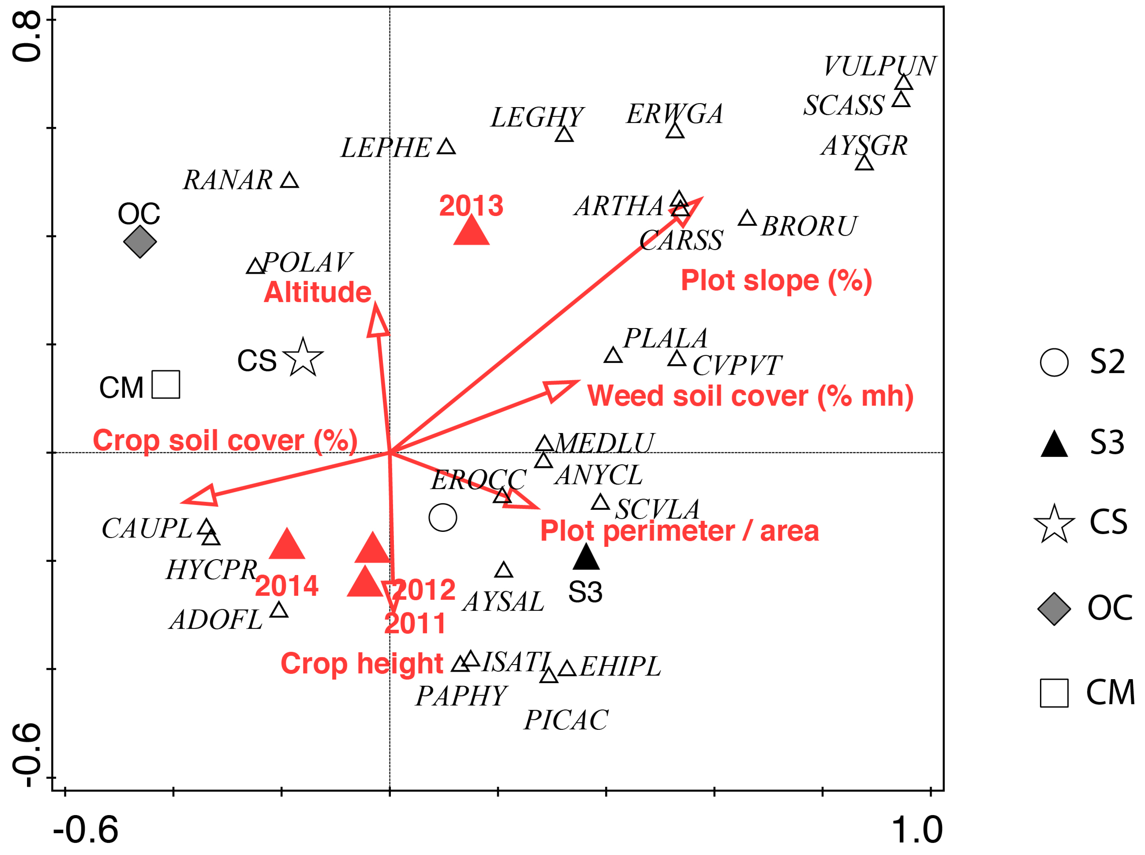
3.2. Weed Community Composition

The amount of species with a frequency exceeding 30% was highest for OC, followed by S2 and S3, and lowest for CM and CS, while the amount of species exceeding 3% of soil cover was quite similar for most of the different crops tending to be slightly higher for S3 (Table 4). It is important to highlight that few species fulfilled both conditions exceeding 30% frequency and 3% soil cover, i.e., few species and should be considered potentially dangerous weed species in the respective crops (Table 5). Including sainfoin in the rotation seems to reduce the number of most dangerous weeds, being lowest in CS and CM and S2 and S3, while OC hosted the most. Interestingly L. rigidum was within the most frequent ones in all crops excluding OC.
Species that were both within the most frequent and most abundant ones that could thus cause most trouble to farmers were P. aviculare and C. arvense in OC, L. rigidum in CM, L. rigidum and P. convolvulus in CS, A. clavatus in S2 and L. rigidum and A. clavatus in S3 (Figure 3, Figure 4, Figure 5, Figure 6 and Figure 7). Also, the group of several Bromus species showed notable abundance values under S2 and S3 but seemed to be nonproblematic in cereal fields, which are generally mouldboard-ploughed in the area. It is also striking that P. rhoeas was within the most frequent species in all crops (a bit less in CS) but showed low abundance rates less than 5% in all cases.
All 10 tested environmental variables had a significant effect on weed species distribution (Table 6). Crop type had the highest influence, with S3 being the crop with the most different weed flora, followed by survey year, slope, altitude, crop height, crop cover, field perimeter/area and weed soil cover (Table 5).
The CCA demonstrates that 2013 is associated to a different weed flora overall than the rest of years (Figure 8) what could be consequence of the high rainfall recorded between October 2012 and May 2013, which was almost double as high than in the other three seasons (Figure 1). Also, flora in S2 and S3 were different to the rest of crops, confirming the hypothesis that weed communities found in sainfoin should not be the same than in cereal.
Altitude and crop height had the opposite influence on weed flora. Soils at higher altitude generally have higher stoniness, which is probably related to lower soil fertility and, concurrently, lower crop height. A certain delay in crop development also occurs at higher altitude due to cooler temperatures but this factor should not be affecting cereal and sainfoin in May, when sampling was conducted. Also crop cover and slope have an opposite influence on weed flora.
Our results (Figure 8) indicate that substantial differences in the presence and abundance of plants species in the weed community composition occurred in the different crops. Therefore, species assemblages in the weed community were significantly influenced not only by local and environmental factors but also by crop type (Table 5). The NMDS analysis (k = 2, nonmetric fit: r2 = 0.95) showed a clear distribution of the sites based on the floristic similarities of the surveyed fields (Figure 9).

3.3. Crop Soil Cover and Height

As these two factors were significantly related to species composition, data was additionally analysed. S3 tended to have least cover than S2 all four years, being statistically lower in 2012 (Table 7). CM and CS tended to have bigger soil cover than S2 and S3 in 2011 and 2012 but not in 2013 and 2014, and OC tended to have lower crop cover than CM. Concerning plant height, similar values were obtained for CM, CS, S2 and S3, but OC had statistically lower plant height than the other sampling years.

3.4. Soil Seedbank

A surprisingly high total seed number was found of seeds belonging to 41 different species in CM and to 57 different species in S3. The total seed number as well as the specific richness tended to be higher for S3 fields than for CM fields (Table 8). Despite differences were not significant, total weed seed richness was 1.3-fold higher for S3 compared to CM, which is lower than in the emerged flora accounting for 1.8-, 2.8-, 2.3- and 2.5-fold increases in years 2011, 2012, 2013 and 2014, respectively (calculated from data partially shown in Table 2). A total of 29 species present in S3 were not found in CM. The most frequent species in S3 fields were Anthemis sp. and Alyssum sp. (31% of the samples) and Medicago sp. (20%). Conversely, 13 species were exclusive for CM fields, with Setaria spp. and Cardaria draba (L.) Desv. being present in 20% of the samples fields, but the rest of species exclusive to CM were found in 10% of the samples, only.
Surprisingly, the most frequent and also the most abundant species were the summer species Polygonum spp. and Amaranthus spp. in both crops (Table 9 and Table 10), and quite scarce seeds of the expected typical winter flora were found.
Species with abundance in the third or fourth position had an irregular distribution with a high standard error (Table 9 and Table 10), but were very common species in the area and in the crops excepting Heliotropium europaeum (L.), which is less frequent. In both crops the values were generally low compared to the dominating seeds of Polygonum and Amaranthus spp.
In some plots, a coincident dominance of Polygonum aviculare L. and of Polygonum convolvulus L. in the emerged flora in May and in the seed bank were found, as well as for Alyssum spp. and Veronica spp. in other fields but, generally, few coincidences existed between the emerged flora in May and the species found in the seedbank (Table 2, Table 3, Table 9 and Table 10).

4. Discussion

4.1. Species Richness and Weed Cover

Following [45], fields with higher species richness will probably be less competitive and less prone to dominance by highly adapted species. Thus, in this study, S2, S3 and OC fields are very probably indicative of hosting a weed flora that is easier to control compared to CM and CS. Curiously, species richness in CS was statistically compared to CM, despite growing sainfoin during three years. In other situations, very rapid changes in weed flora have been found in cereal fields e.g., due to specific herbicide management, after only four years [46]. Thus, in the present study, the higher biodiversity recorded in sainfoin diminishes rapidly after sowing again winter cereal.
The rainfall in the whole cropping season, i.e., between October and May seasons 2012–2013 and 2010–2011, should have been the most favourable from a rainfall point of view. Considering only spring rainfall, again more crop growth should have been expected for springs 2013 and 2011. In fact, the highest species richness was found in 2013, followed by 2011, which could be caused by a higher crop competition and to higher species diversity due to increased rainfall those years.
Concerning weed cover, low and high rainfall, recorded in spring 2014 and 2013, respectively, could also explain the lower and higher weed cover found those years (Table 3). Occasional herbicide use in CM and CS in the area is probably the main cause for high weed cover in the cereal crops, which only tended to be lower than in the S2 and S3 fields. Moreover, taking into account the found weed cover values, most sainfoin fields would have been considered as ordinary or third quality [36], despite that weeds in sainfoin do not substantially harm, as far as they add biomass to the pasture and are generally used for on-farm use and are often not commercialised [13].
The results of lower crop cover in S3 compared to S2 suggest a decay of the crop as shown by other authors [4,46,47] (Table 6). The lack of significant differences in crop cover between cereals and sainfoin at flowering/earing shows that both types of crops probably compete similarly with weeds at this stage. Concerning crop height, the only significant differences concerned OC, which was smaller than the rest of sampled crops, very probably due to organic fertilisation instead of chemical dressing. Thus, differences in weed cover in the different crops could not be clearly explained with these two parameters determined at flowering/tillering. However, very probably, cereal covers the soil faster than sainfoin, thus competing better against weeds despite high-density sown sainfoin that may also be able to reduce weeds. Therefore, a more detailed crop cover and height description during the whole cropping cycle would be interesting to shed more light upon this topic included as a sainfoin breeding objective.

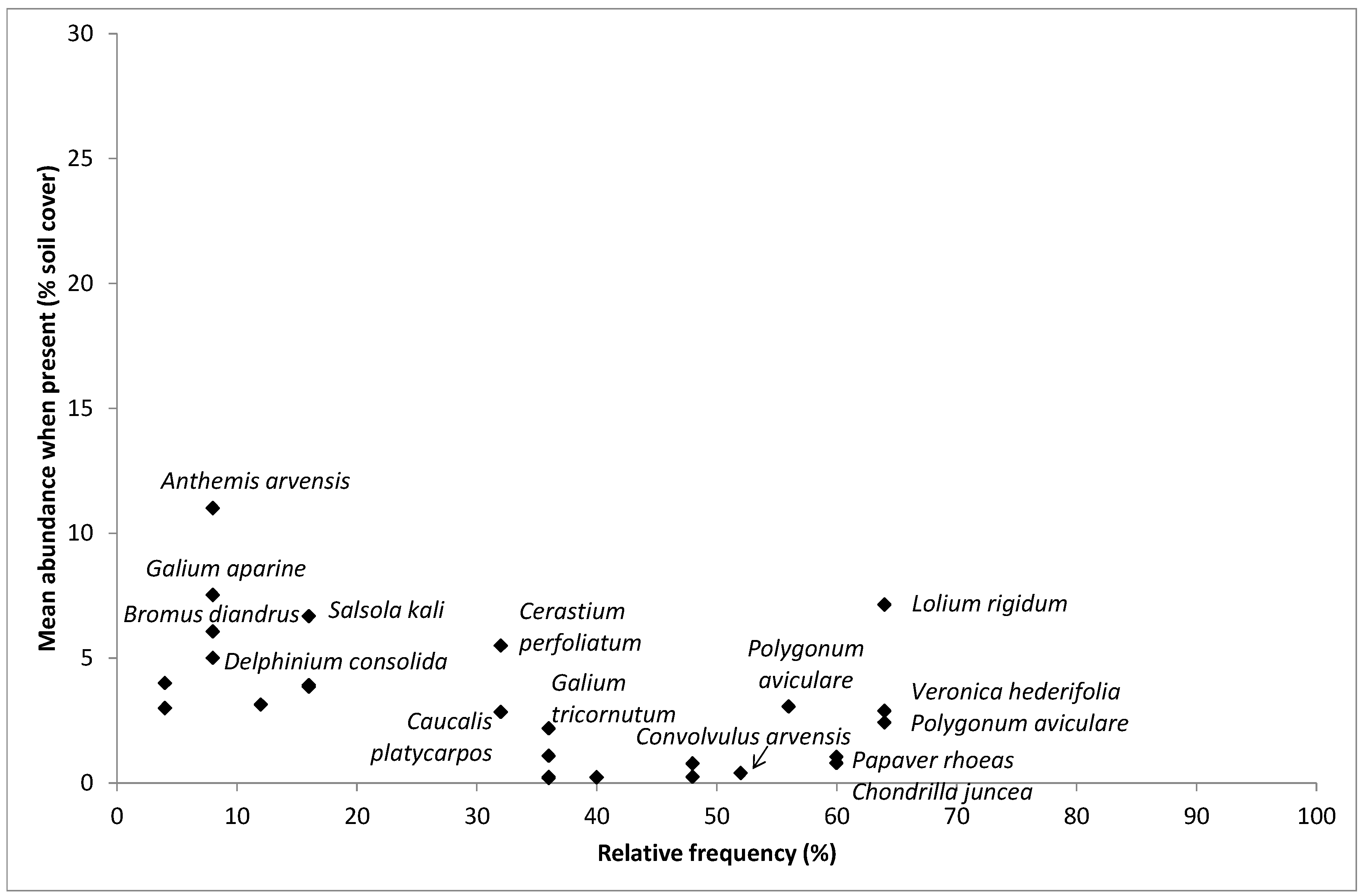
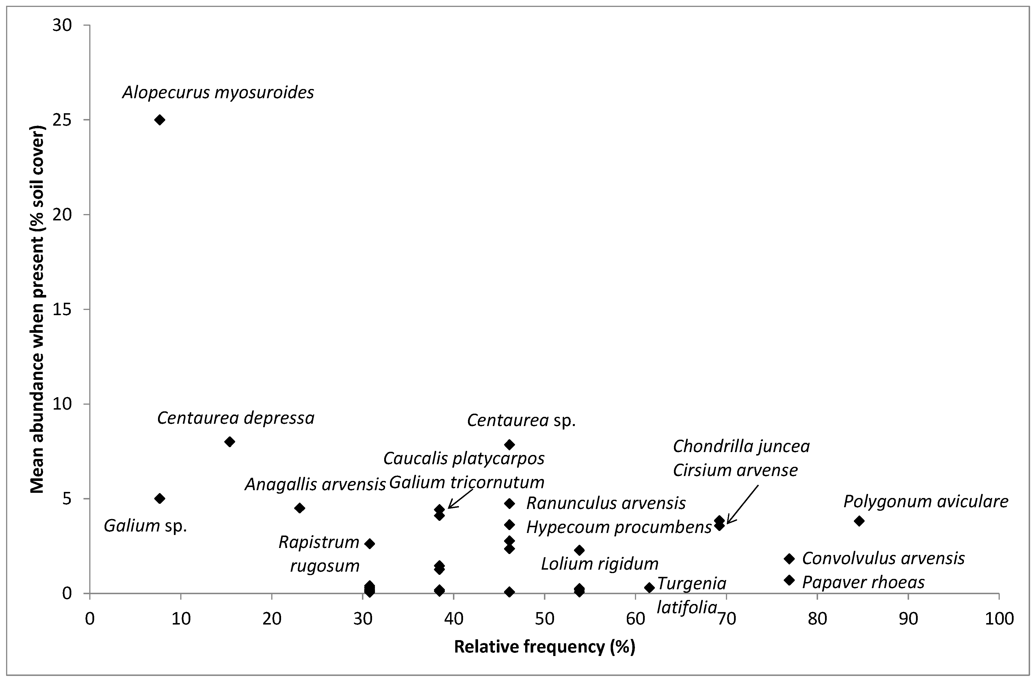
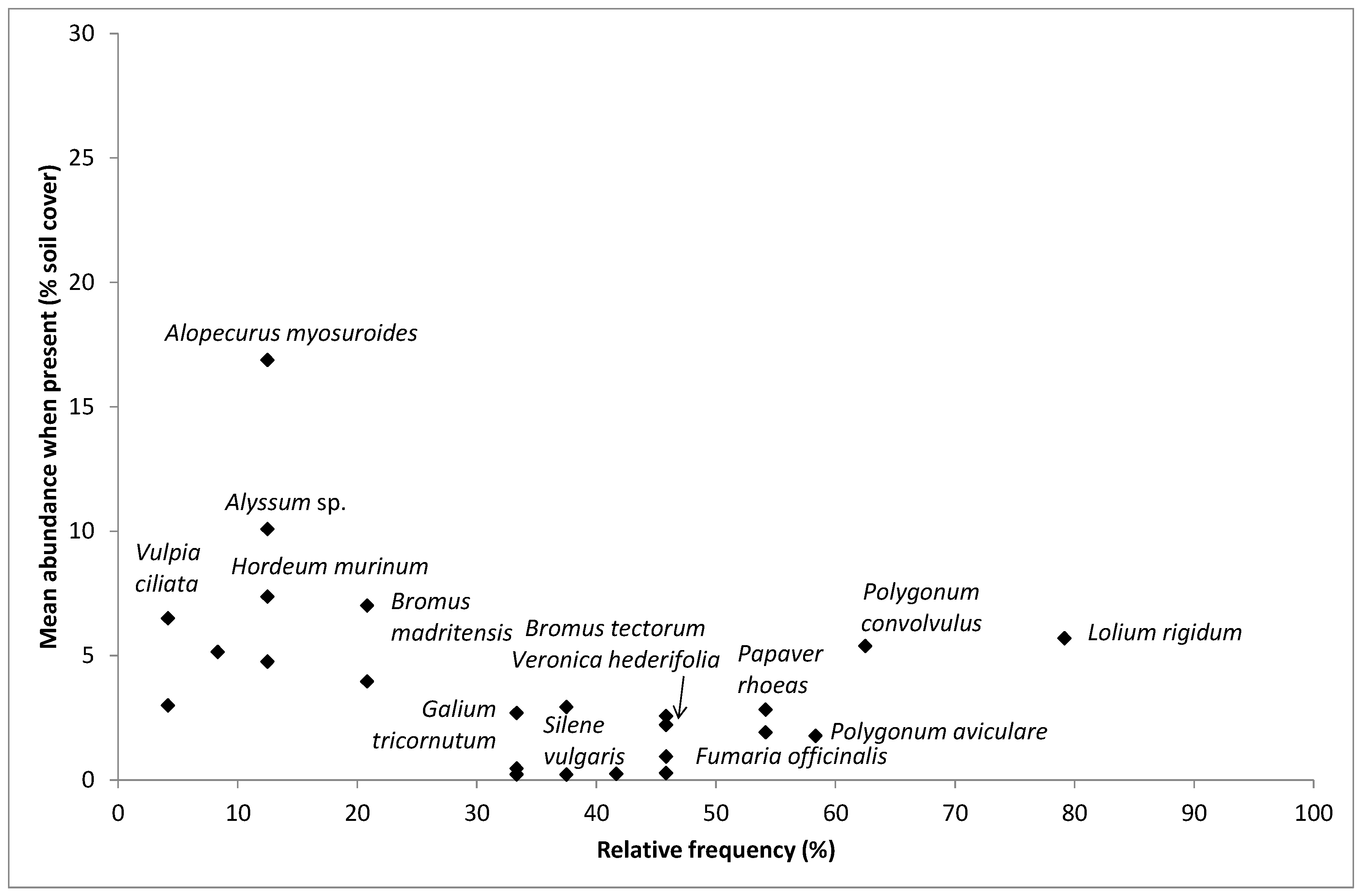
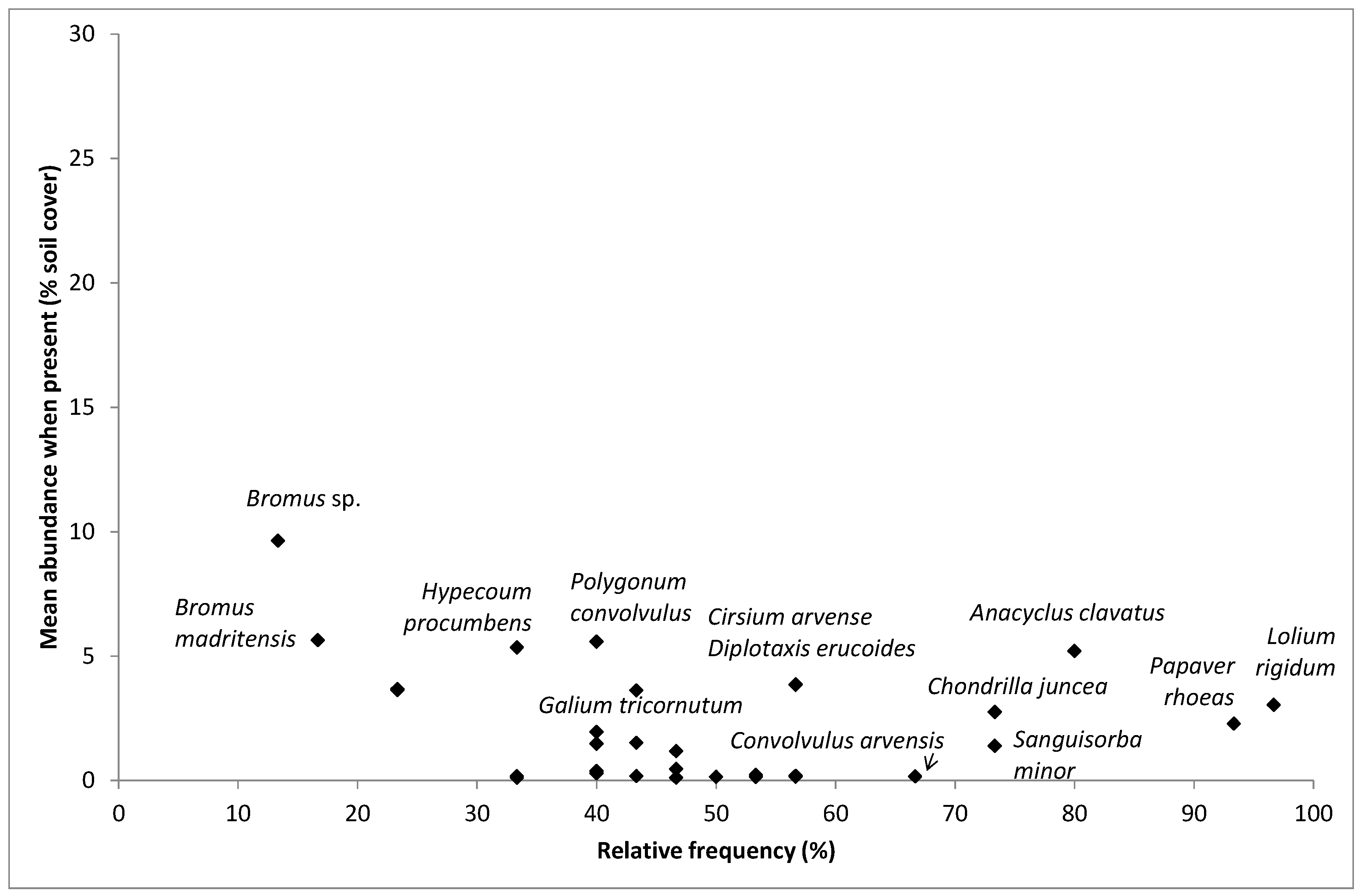
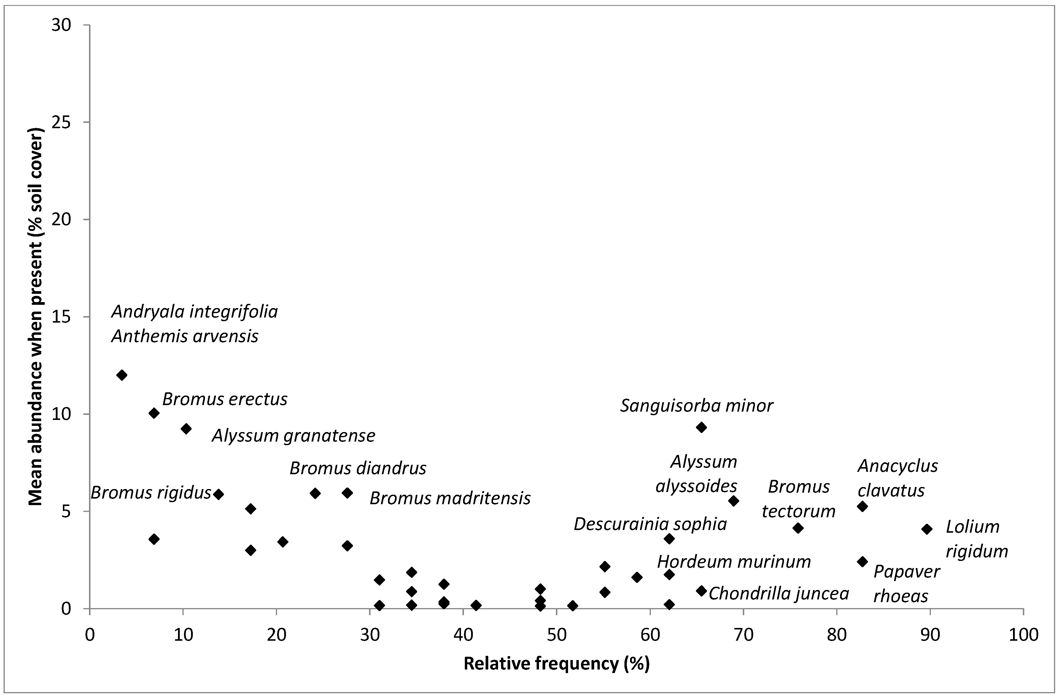
4.2. Most Frequent and Most Abundant Species

It is not surprising that more weed species were very abundant in S3 compared to the other crops where no weed control methods have been adopted except for mowing or grazing for three years. However, this fact cannot be considered dramatic as no toxic plants were identified and weeds are edible for sheep too. The control methods used in OC seemed to be effective enough to reduce the number of potentially troublesome weed species down to a similar value than in the other cereal fields handled conventionally. The higher amount of species being frequent in OC and S2 and S3 fields is probably related to the more extensive management of these fields as also found by [48,49] in organically managed cereal fields compared to conventional ones.
Lower L. rigidum abundance in S2 and S3 may be because this grass also finds good conditions for germinating in sainfoin, howeverthe seed bank may gradually decrease because mowing in May makes resowing of this species possible only for early-ripening individuals. Highest abundance of L. rigidum in CM may be due to the good response of this species to fertilisation and semi-intensive conditions as well as its ability of developing herbicide resistance documented in other areas of Aragon since 1997 [50]. Moreover, this species is known to be one of the main weeds in cereal fields all over the Aragon region [32] and is probably well-adapted to any winter-growing crop excepting the low-intensity OC systems. In fact, other studies have shown the difficulty in controlling this species by mechanical and cultural ways, which are the main control tools in organic management [51].
The fact that P. rhoeas was within the most frequent species in all crops is consistent with other work demonstrating its good adaptation to periodic mouldboard ploughing corresponding to the situations in CM, OC and CS [52] and its ability to prosper at the same time under no-tillage [53], which corresponds to the situations in S2 and S3. P. rhoeas can also find good conditions for germinating in clear stands what may occur in dry years in any of the crops. The present results confirm the ability of this species to be dominant in several situations.
Unexpectedly several of the most troublesome weeds with high abundance and frequency were coincident in OC and S2, i.e., C. arvense, H. procumbens and G. tricornutum being not found in those high proportions in the other crops (Table 3). Lack of herbicide use for broadleaved weed species control and lack of mineral fertilisation in OC and S2 might be the responsible of the increase of these species. Furthermore, auxin-like herbicides used in CM usually control the first two species efficiently while specific herbicides might be used in severe G. tricornutum infestations.
The Integrated Pest Management guide published by the Spanish Ministry of Agriculture considers 2% as the threshold inside a cereal field to decide whether or not to conduct a treatment for the sum of the found weeds or for some of them individually [21]; Avena sterilis L., Bromus diandrus Roth, L. rigidum and Papaver rhoeas L. being the most troublesome weeds in cereal [32]. Similarly, in Germany the general economic threshold inside a cereal field has been established in 5–10% for broad-leaved species [54]. In the present data, abundance exceeding 10% was found in a few cases only, i.e., Alopecurus myosuroides Huds. in OC, CS and S2; Anthemis arvensis L. in CM and S3; Andryala integrifolia L. and B. erectus Huds. in S3; and Xanthium spinosum L. in S2. The only cases exceeding 10% in both parameters were Alyssum spp. and A. myosuroides under CS (Figure 3, Figure 4, Figure 5, Figure 6 and Figure 7). Alyssum species were abundant and frequent in S2 and S3 and could infest the subsequent cereal, despite the values were much smaller in CS after ploughing. However, its small size and short cycle may cause very little competition. Opposite, A. myosuroides did not seem to increase due to growing sainfoin; as this species reached higher values in CS than in S2 or S3 (7% frequency and soil cover of 10% and 0.3% in S2 and S3, respectively).

4.3. Species Composition

In terms of local landscape structure, the landscape metrics related with the shape of the fields affected species composition. In other studies, irregular shaped fields with higher perimeter-area ratio than regular shaped ones provide a higher amount of potential source habitat for arable weeds that can spread and colonise in the inner field positions [55,56].
Concurrently, some of these species have been classified as rare arable species, which refuge in fields characterised by low inputs and low productivity [55]. On the other hand, the absence of soil disturbance in sainfoin fields implies that species such as Ranunculus arvensis L., Caucalis platycarpos L. and Adonis flammea Schleich. ex Steud. (Table 3, Figure 8) become less common or absent. It is known that the absence of regular soil disturbance in crop fields could have increased the establishment of certain weeds, such as perennials or winter annuals, at the expense of the highly specialised rare arable plants. Therefore, regular soil disturbance is crucial to promote emergence and build-up of rare arable plants.
Furthermore, from a functional point of view, rare arable plants share a ‘rare weed trait syndrome’ that helps to explain their decline in different parts of Europe based on their similar response to management factors [57]. However, some studies highlight that the rarity of these species can be the result of specific interactions between seed traits and soil disturbance, particularly in semi-arid cereal fields in Mediterranean Europe [56].
The NMDS revealed that plant assemblages respond to the difference intensification of the crop types, leading to a biotic homogenisation within fields subjected to the same management [55,58]. Stability in sainfoin field seems to favour a set of species which become dominant in absence of soil disturbance, which can undergo changes in species richness and diversity (Table 1 and Table 2).

4.4. Soil Seedbank

In the soil seedbank at time of sampling (May) many species were at flowering stage previous to new seed shed so that the expected seeds in the seedbank should mainly belong to short-cycle species such as Veronica spp., Stellaria media (L.) Vill., etc., or from those species able to shed seeds in previous summers or autumns.
A possible explanation for lack of winter flora seeds in the sainfoin fields is that mowing and pasturing of the crop causes that seed bank depletion by impeding the plants flowering in May to finish their cycle. This would support the farmers’ perception that sainfoin cleans the field from weeds harmful in cereal despite hosting many weeds [28]. This way, seeds of species germinating in spring-summer and finishing the live cycle after mowing or pasturing as Amaranthus spp. would be favoured. Due to their prostrated growth habit possibly most of the Polygonum plants survive the moving and regrow afterwards while most of the Amaranthus plants probably germinated after mowing. Also those species producing new shoots after the crop exploitation, e.g., species of the Poaceae family, could benefit from this crop provided that they are capable to shed seeds after mowing or grazing. Moreover, seeds from Amaranthus spp. are long-lived seeds able to germinate 7% 12 years after burial at 20 cm depth [59], Polygonum aviculare and P. convolvulus showed a seed viability decline pattern of a rapid loss of viability in the first 9.7 years after burial, but with a slower rate of decline afterwards with a slow proportion of seeds still remaining viable 19.7 years after burial [58]. These seeds are possibly not especially attractive for the local seed predators who had probably gathered many Poaceae seeds in the sampling moment [60].
On the other hand, it is known that ant populations increase seed predation activity with decreasing soil tillage [61], which was confirmed in the present data set by the abundance of ant rests found in the elutriator samples. Once the colonies are established they gather the seeds very rapidly burying them in the soil. These animals efficiently remove weed seeds being those of Poaceae, such as L. rigidum and Bromus spp. [62], which are abundant in many sainfoin fields but scarce in the seed bank of the same fields. It is thus hypothesised that in May most of those seeds produced in the previous summer attractive for ants had already been removed and the new seed rain has not yet occurred.
The abundance of seeds of the summer annuals in the CM fields could be explained by the fact that after mowing in July no other crop is grown until the next cereal is sown in October-November and that these species are able to use moisture from summer storms to complete their cycle.
Curiously few coincidences between emerged flora and seed bank were found. A possible explanation for this is that species like Bromus spp., which dominated in the aboveground vegetation, generate seeds that do not survive long time in the soil [63]. Thus as seed rain of the year had not yet occurred, it would be difficult to find seeds from the previous year. Also wind dispersion, for example of the Compositae species Chondrilla juncea and Lactuca serriola and seed predation by birds can have contributed in the little coincidence between the emerged flora and the seed bank. In other cases the reason might be have been that the species was yet not present in May because the emergence period is subsequent to the May sampling (e.g., Amaranthus spp.).
Additionally, a known drawback of the soil seedbank technique is the difficulty of sampling a representative amount of soil, among others [64]. Thus, it is possible that some species were not detected with this seed bank sampling technique due to collecting a too small soil size. Opposite, the description of the emerged flora in May focuses on species that could be dangerous for winter cereal, the detection of small-sized species, of those finishing the cycle early in spring and of species with summer cycle developing after the mowing or after pasturing the sainfoin as Amaranthus spp. are underestimated in these visual assessments in spring. Both sampling methods are thus incomplete but complementary and, in both cases, it has been found that there is a tendency of higher diversity in S3 plots compared to CM as well as a reduction of the most harmful species in cereal such as L. rigidum and P. rhoeas, which were only found at insignificant amount in the sainfoin fields seed bank.

Author Contributions

A.C. and S.M. conceived and designed the surveys; A.C., A.I.M., S.M., J.A. and G.P. performed the surveys; A.C., S.M. and X.-O.S.-S. analysed the data; A.C. wrote the paper with assistance of X.-O.S.-S. and J.A.

Funding

This work was financed by the Spanish Ministry of Science and Innovation, project AGL2010-22084-C02-02.

Acknowledgments

Thanks to R. Gurucharri and to the car drivers of the Aragon Government for their collaboration. We acknowledge the Weed Science and Plant Ecology Group of the University of Lleida for allowing us to use the seed elutriator and A. Clavería for her help in the surveys. Thanks to M. Mas and A.M.C. Verdú for their help in identifying seeds.

Conflicts of Interest

The authors declare no conflict of interest and the founding sponsors had no role in the design of the study; in the collection, analyses, or interpretation of data; in the writing of the manuscript, and in the decision to publish the results.

References

  1. Kallenbach, R.L.; Matches, A.G.; Mahan, J.R. Sainfoin regrowth declines as metabolic rate increases with temperature. Crop Sci. 1996, 36, 91–97. [Google Scholar] [CrossRef]
  2. Meyer, D.W.; Badaruddin, M. Frost tolerance of ten seedling legume species at four growth stages. Crop Sci. 2001, 41, 1838–1842. [Google Scholar] [CrossRef]
  3. Molle, G.; Decandia, M.; Solter, U.; Greef, J.M.; Rochon, J.J.; Sitzia, M.; Hopkins, A.; Rook, A.J. The effect of different legume-based swards on intake and performance of grazing ruminants under Mediterranean and cool temperate conditions. Grass Forage Sci. 2008, 63, 513–530. [Google Scholar] [CrossRef]
  4. Mora-Ortiz, M.; Smith, L.M.J. Onobrychis viciifolia: A comprehensive literatura review of its histroy, etymology, taxonomy, genetics, agronomy and botany. Plant Genet. Resour.-C 2018, 16, 403–418. [Google Scholar] [CrossRef]
  5. Carbonero, C.H.; Mueller-Harvey, I.; Brown, T.A.; Smith, L. Sainfoin (Onobrychis viciifolia): A beneficial forage legume. Plant Genet. Resour.-C 2011, 9, 70–85. [Google Scholar] [CrossRef]
  6. Naseri, B.; Alizadeh, M.A. Climate, powdery mildew, sainfoin resistance and yield. J. Plant. Pathol. 2017, 99, 619–625. [Google Scholar]
  7. Hwang, D.F.; Gaudet, D.A. Effects of plant age and late-season hardening on development of resistance to winter crown rot in first-year sainfoin (Onobrychis viciifolia). J. Plant. Dis. Protect. 1999, 106, 188–197. [Google Scholar]
  8. Tozlu, G.; Hayat, R. Biology of Cholorophorus robustior Pic, 1900 (Coleoptera: Cerambycidae), a new record and a new sainfoin (Onobrychis sativa Lam.) pest for Turkey. Isr. J. Zool. 2000, 46, 201–206. [Google Scholar] [CrossRef]
  9. Sintim, H.Y.; Adjesiwor, A.T.; Zheljazkov, V.D.; Islam, M.A.; Obour, A.K. Nitrogen application in sainfoin under rain-fed conditions in Wyoming: Productivity and cost implications. Agron. J. 2016, 108, 294–300. [Google Scholar] [CrossRef]
  10. MAPAMA. Anuario de Estadísticas. Avance 2016. Ministerio de Agricultura y Pesca, Alimentación y Medio Ambiente. 2017. Available online: http://www.mapama.gob.es/estadistica/pags/anuario/2016-Avance/avance/AvAE16.pdf. (accessed on 26 June 2017).
  11. Delgado, I.; Andrés, C.; Sin, E.; Ochoa, M.J. Estado actual del cultivo de la esparceta (Onobrychis viciifolia Scop.). Encuesta realizada a agricultores productores de semilla. Pastos 2002, 32, 235–247. [Google Scholar]
  12. BOA. Boletín Oficial de Aragon. 2015. Available online: http://www.boa.aragon.es/cgi-bin/EBOA/BRSCGI?CMD=VEROBJ&MLKOB=840111824848 (accessed on 12 September 2016).
  13. Marí, A.I.; Cirujeda, A.; Murillo, S.; Pardo, G.; Aibar, J. Resultado de las encuestas realizadas sobre el cultivo de esparceta (Onobrychis viciifolia Scop.) y su efecto sobre las malas hierbas en la zona de Teruel. In Proceedings of the XV Congress of the Spanish Weed Science Society (SEMh), Sevilla, Spain, 19–22 October 2015. [Google Scholar]
  14. Legendre, H.; Hoste, H.; Gidenne, T. Nutritive value and anthelmintic effect of sainfoin pellets fed to experimentally infected growing rabbits. Animal 2017, 11, 1464–1471. [Google Scholar] [CrossRef]
  15. Bhattarai, S.; Coulman, B.; Biligetu, B. Sainfoin (Onobrychis viciifolia Scop.): Renewed interest as a forage legume for western Canada. Can. J. Plant Sci. 2016, 96, 748–756. [Google Scholar] [CrossRef]
  16. Huyen, N.T.; Desrues, O.; Alferink, S.J.J.; Zandstra, T.; Verstegen, M.W.A.; Hendriks, W.H.; Pellikaan, W.F. Inclusion of sainfoin (Onobrychis viciifolia) silage in dairy cow rations affects nutrient digestibility, nitrogen utilization, energy balance, and methane emissions. J. Dairy Sci. 2016, 99, 3566–3577. [Google Scholar] [CrossRef]
  17. Heckendorn, F.; Werne, S.; Maurer, V.; Perler, E.; Amsler, Z.; Probst, J.; Zaugg, C.; Krenmeyr, I. Sainfoin—New data on anthelmintic effects and production in sheep and goats. Planta Med. 2013, 79, 1125. [Google Scholar] [CrossRef]
  18. Saratsis, A.; Voutzourakis, N.; Theodosiou, T.; Stefanakis, A.; Sotiraki, S. The effect of sainfoin (Onobrychis viciifolia) and carob pods (Ceratonia siliqua) feeding regimes on the control of lamb coccidiosis. Parasitol. Res. 2016, 115, 2233–2242. [Google Scholar] [CrossRef]
  19. Baldinger, L.; Hagmuller, W.; Minihuber, U.; Matzner, M.; Zollitsch, W. Sainfoin seeds in organic diets for weaned piglets utilizing the protein-rich grains of a long-known forage legume. Ren. Agric. Food Syst. 2016, 31, 12–21. [Google Scholar] [CrossRef]
  20. Kashevarov, N.I.; Polyudina, R.I.; Rozhanskaya, O.A.; Jeleznov, A.V. Sainfoin (Onobrychis Mill.) breeding for forage production in Siberia. Kormoproizvodstvo 2013, 9, 22–24. [Google Scholar]
  21. Aufrere, J.; Theodoridou, K.; Baumont, R.; Baumont, R. Agronomic and nutritional value of sainfoin. Fourrages 2013, 213, 63–75. [Google Scholar]
  22. Marinov-Serafimov, P.; Golubinova, I.; Vasileva, V. Dynamics and distribution of weed species in weed associations. Indian J. Agric. Sci. 2019, 89, 105–110. [Google Scholar]
  23. Liu, Z.; Baines, R.N.; Lane, G.P.F.; Davies, W.P. Survival of plants of common sainfoin (Onobrychis viciifolia Scop.) in competition with two companion grass species. Grass Forage Sci. 2010, 65, 11–14. [Google Scholar] [CrossRef]
  24. Kempf, K.; Grieder, C.; Walter, A.; Widmer, F.; Reinhard, S.; Kolliker, R. Evidence and consequences of self-fertilisation in the predominantly outbreeding forage legume Onobrychis viciifolia. BCM Genet. 2015, 16. [Google Scholar] [CrossRef]
  25. Delgado, I.; Salvia, J.; Buil, I.; Andrés, C. The agronomic varibaility of a collection of sainfoin accessions. Span. J. Agric. Res. 2008, 63, 401–407. [Google Scholar] [CrossRef]
  26. Sebastià, M.; Palero, N.; De Bello, F. Changes in Management modify agro-diversity in sainfoin swards in the Eastern Pyrenees. Agron. Sustain. Dev. 2011, 341, 533–540. [Google Scholar]
  27. Cirujeda, A.; Marí, A.; Murillo, S.; Aibar, J. La flora arvense en el cultivo de la esparceta (Onobrychis viciifolia L.) aumenta la biodiversidad vegetal. In Proceedings of the XIV Congress of the Spanish Weed Science Society (SEMh), Valencia, Spain, 5–7 November 2013; Osca, J.M., Gómez de Barreda, D., Castell, V., Pascual, N., Eds.; Universitat Politécnica de València: Valencia, Spain, 2013; pp. 31–35. [Google Scholar]
  28. Anderson, R.L. Managing weeds with a dualistic approach of prevention and control. A review. Agron Sustain. Dev. 2007, 27, 13–18. [Google Scholar] [CrossRef]
  29. BBCH Working Group. Compendium of Growth Stage Identification Keys for Mono- and Dicotyledonous Plants. Extended BBCH Scale; BBA, BSA, IGZ, IVA, AGREVO, BASF, Bayer, Novartis, Eds.; Allcomm Business Communication: Bezug, Germany, 1997. [Google Scholar]
  30. Walker, K.J.; Critchley, C.N.R.; Sherwood, A.J.; Large, R.; Nuttall, P.; Hulmes, S.; Rose, R.; Mountford, J.O. The conservation on arable plants on cereal field margins: An assessment of new agri-environment scheme options in England, UK. Biol. Conserv. 2007, 136, 260–270. [Google Scholar] [CrossRef]
  31. Marnotte, P. Influence des facteurs agroécologiques sur le developpement des mauvaises herbes en climat tropical humide. In Proceedings of the 1984 7ème Colloque International Ecologie, Biologie et Systematique des Mauvaises Herbes, Paris, France, 9–11 October 1984; pp. 183–188. [Google Scholar]
  32. Cirujeda, A.; Aibar, J.; Zaragoza, C. Remarkable changes of weed species in Spanish cereal fields from 1976 to 2007. Agron. Sustain. Dev. 2011, 31, 675–688. [Google Scholar] [CrossRef]
  33. SigPac database, 3.2. Available online: http://sigpac.mapama.gob.es/fega/visor/ (accessed on 28 August 2014).
  34. Reinhardt, T.; Leon, R.G. Extractable and germinable seedbank methods provide different quantifications of weed communities. Weed Sci. 2018, 66, 715–720. [Google Scholar] [CrossRef]
  35. Hanf, M. The Arable Weeds of Europe with Their Seedlings and Seeds; BASF: Ludwigshafen, Germany, 1983; pp. 1–494. [Google Scholar]
  36. Holm-Nielsen, C. Frø fra det Dyrkede Land. 258 Plantearter; Forskningscenter Flakkebjerg: Slagelse, Denmark, 1998; pp. 1–178. ISBN 87-984996-0-2. [Google Scholar]
  37. Viaggiani, P. Erbe Spontanee e Infestanti: Technique di Risonoscimento: Dicotiledoni; Bayer: Milano, Italy, 1990; pp. 1–271. [Google Scholar]
  38. MAPAMA (Ministerio de Agricultura y Pesca, Alimentación y Medio Ambiente). Guía de Gestión Integrada de Plagas. Cereales de Invierno. 2015. Available online: http://www.magrama.gob.es/es/agricultura/temas/sanidad-vegetal/productos-fitosanitarios/guias-gestion-plagas/ (accessed on 12 September 2016).
  39. Lloveras, J.; Melines, M.A. La calidad en la alfalfa. Posibles clasificaciones. Vida Rural 2015, 212, 36–40. [Google Scholar]
  40. Magurran, A.E. Ecological Diversity and Its Measurement; Princeton University Press: Princeton, NJ, USA, 1988; pp. 145–149. ISBN 978-0691084916. [Google Scholar]
  41. SAS Institute. SAS Systems for Linear Models; SAS Series in Statistical Applications; SAS Institute: Cary, NC, USA, 1991. [Google Scholar]
  42. R Core Team. R: A Language and Environment for Statistical Computing; R Foundation for Statistical Computing: Vienna, Austria, 2014; Available online: http://www.R-project.org/ (accessed on 20 February 2019).
  43. Smilauer, P.; Leps, J. Multivariate Analysis of Ecological Data using Canoco 5, 2nd ed.; Cambridge University Press: Cambridge, UK, 2014; pp. 1–362. ISBN 978-0-521-89108-0. [Google Scholar]
  44. La garita del Jiloca. Available online: http://tiempocalamocha.blogspot.com.es (accessed on 5 June 2017).
  45. Storkey, J.; Neve, P. What good is weed diversity? Weed Res. 2018, 58, 239–243. [Google Scholar] [CrossRef]
  46. Mayerová, M.; Mikulka, J.; Soukup, J. Effects of selective herbicide treatment on weed community in cereal crop rotation. Plant Soil Environ. 2018, 64, 413–420. [Google Scholar] [CrossRef]
  47. Stevovic, V.; Stanisavljevic, R.; Djukic, D.; Djurovic, D. Effect of row spacing on seed and forage yield in sainfoin (Onobrychis viciifolia Scop.) cultivars. Turk. J. Agric. For. 2012, 36, 35–44. [Google Scholar]
  48. Chamorro, L.; Masalles, R.M.; Sans, F.X. Arable weed decline in Northeast Spain: Does organic farming recover functional biodiversity. Agric. Ecosyst. Environ. 2016, 223, 1–9. [Google Scholar] [CrossRef]
  49. Romero, A.; Chamorro, L.; Sans, F.X. Weed diversity in crop edges and inner fields of organic and conventional dryland Winter cereal crops in NE Spain. Agric. Ecosyst. Environ. 2008, 124, 97–104. [Google Scholar] [CrossRef]
  50. Sopeña, J.M.; Zaragoza, C. Principales problemas de malas hierbas y herbicidas plantados durante 1997 en Aragon. In Proceedings of the XVII Meeting of the Spanish Weed Working Group, Santa Cruz de Tenerife, Spain, 3–6 March 1998; p. 118. [Google Scholar]
  51. Cirujeda, A.; Taberner, A. Cultural control of herbicide-resistant Lolium rigidum Gaud. populations in winter cereal in Northeastern Spain. Span. J. Agric. Res. 2009, 7, 146–154. [Google Scholar] [CrossRef]
  52. Cirujeda, A.; Recasens, J.; Taberner, A. Effect of ploughing and harrowing on a herbicide resistant corn poppy (Papaver rhoeas) population. Biol. Agric. Hortic. 2003, 21, 231–246. [Google Scholar] [CrossRef]
  53. Navarrete, L.; Sánchez, M.J.; Alarcón, R.; Hernanz, J.L.; Sánchez-Girón, V. Respuesta de los cultivos y la vegetación arvense a la reducción de la fertilización y al tipo de laboreo en sistemas cerealistas de secano. In Proceedings of the XV Congress of the Spanish Weed Science Society (SEMh), Sevilla, Spain, 19–22 October 2015. [Google Scholar]
  54. Gerowitt, B.; Heitefuss, R. Weed economic thresholds in cereals in the Federal Republic of Germany. Crop Prot. 1990, 9, 323–331. [Google Scholar] [CrossRef]
  55. Solé-Senan, X.O.; Juárez-Escario, A.; Conesa, J.A.; Torra, J.; Royo-Esnal, A.; Recasens, J. Plant diversity in mediterranean cereal fields: Unraveling the effect of landscape complexity on rare arable plants. Agric. Ecosyst. Environ. 2014, 185, 221–230. [Google Scholar] [CrossRef]
  56. Solé-Senan, X.O.; Juárez-Escario, A.; Robleño, I.; Conesa, J.A.; Recasens, J. Using the response-effect trait framework to disentangle the effects of agricultural intensification on the provision of ecosystem services by mediterranean arable plants. Agric. Ecosyst. Environ. 2017, 247, 255–264. [Google Scholar] [CrossRef]
  57. Pinke, G.; Gunton, R. Refining rare weed trait syndromes along arable intensification gradients. J. Veg. Sci. 2014, 25, 978–989. [Google Scholar] [CrossRef]
  58. Solé-Senan, X.O.; Juárez-Escario, A.; Conesa, J.A.; Recasens, J. Plant species, functional assemblages and partitioning of diversity in a mediterranean agricultural mosaic landscape. Agric. Ecosyst. Environ. 2018, 256, 163–172. [Google Scholar] [CrossRef]
  59. Burnside, O.C.; Wilson, R.G.; Weisberg, S.; Hubbard, K.G. Seed longevity of 41 weed species buried 17 years in Eastern and Western Nebraska. Weed Sci. 1996, 44, 74–86. [Google Scholar]
  60. Conn, J.S.; Beattle, K.L.; Blanchard, A. Seed viability and dormancy of 17 weed species after 19.7 years of burial in Alaska. Weed Sci. 2006, 54, 464–470. [Google Scholar] [CrossRef]
  61. Baraibar, B.; Torra, J.; Westermann, P. Harvester ant (Messor barbarus (L.)) density as related to soil properties, topography and management in semi-arid cereals. Appl. Soil Ecol. 2011, 51, 60–65. [Google Scholar] [CrossRef]
  62. Baraibar, B.; Carrión, E.; Recasens, J.; Westermann, P.R. Unravelling the process of weed seed predation: Developing options for better weed control. Biol. Control 2011, 56, 85–90. [Google Scholar] [CrossRef]
  63. Harradine, A.R. Seed longevity and seedling establishment of Bromus diandrus Roth. Weed Res. 1986, 26, 173–180. [Google Scholar] [CrossRef]
  64. Haring, S.C.; Flessner, M.L. Improving soil seed bank management. Pest Manag. Sci. 2018, 74, 2412–2418. [Google Scholar] [CrossRef] [PubMed]
Figure 1. Map showing the surveyed fields. S2: sainfoin in the second year, S3: sainfoin in the third year, CS: sainfoin after cereal, OC: organic cereal, CM: cereal monocrop. The rest of OC fields were located in Fuentes Calientes, approximately 20 km south and are not included in the Figure to facilitate visualisation.
Agronomy 09 00134 g001
Figure 2. Mean, maximum and minimum monthly temperatures (°C) and monthly rainfall (mm) of the data collected in the four survey years in Calamocha (Spain) [44].
Agronomy 09 00134 g002
Figure 3. Species relative frequency and mean abundance when present in cereal monocrop fields (CM). Data of years 2011–2014 pooled together. Named species are the most abundant and most frequent ones.
Agronomy 09 00134 g003
Figure 4. Species relative frequency and mean abundance when present in organic cereal fields (OC). Data of years 2013–2014 pooled together. Named species are the most abundant and most frequent ones.
Agronomy 09 00134 g004
Figure 5. Species relative frequency and mean abundance when present in cereal fields after cropping sainfoin (CS). Data of years 2011–2014 pooled together. Named species are the most abundant and most frequent ones.
Agronomy 09 00134 g005
Figure 6. Species relative frequency and mean abundance when present in sainfoin fields in their second year of establishment (S2). Data of years 2011–2014 pooled together. Named species are the most abundant and most frequent ones.
Agronomy 09 00134 g006
Figure 7. Species relative frequency and mean abundance when present in sainfoin fields in their third year of establishment (S3). Data of years 2011–2014 pooled together.
Agronomy 09 00134 g007
Figure 8. CCA analysis graph. CM: cereal monocrop, CS: cereal after sainfoin, OC: organic cereal, S2: sainfoin second year, S3: sainfoin third year.
Agronomy 09 00134 g008
Figure 9. Nonmetric multidimensional scaling ordination based on the floristic similarities depending on the crop type of 108 fields.
Agronomy 09 00134 g009
Table 1. Results of the Analysis of Variance (ANOVA) analysis of species richness and Shannon index.
Factorsp-Value (Species Richness)p-Value (Shannon)
Year0.02270.3997
Crop<0.0001<0.0001
Year*Crop0.45820.203
Table 2. Mean weed species richness and Shannon diversity index in the different crops. CM: cereal monocrop, CS: cereal after sainfoin, OC: organic cereal, S2: sainfoin second year, S3: sainfoin third year.
CropCMCSOCS2S3
Shannon Index1.26 bc1.19 c1.23 c1.38 a1.35 ab
Species richness13.9 c17.7 c24.0 b31.6 a33.1 a
Year2011201220132014
Species richness25.1 xy21.4 y26.9 x21.8 y
Different letters refer to significant differences in each column following Student–Newman–Keuls (p < 0.05).
Table 3. Mean weed cover (%) in the different crops. CM: cereal monocrop, CS: cereal after sainfoin, OC: organic cereal, S2: sainfoin second year, S3: sainfoin third year.
Crop2011201220132014
CM20.7 a24.3 c33.3 a14.5 a
CS16.8 a41.7 bc41.7 a20.4 a
OC--46.7 a23.6 a
S242.5 a59.2 ab41.7 a11.4 a
S344.4 a71.7 a55.7 a27.5 a
Different letters within each year refer to significant differences following the nonparametric Kruskal–Wallis test and Wilcoxon test (p < 0.05).
Table 4. Number of species with highest frequency and soil cover in the different crops in all four sampling years. CM: cereal monocrop, CS: cereal after sainfoin, OC: organic cereal, S2: sainfoin second year, S3: sainfoin third year.
CropNumber of Species with Frequency >30%Number of Species with Soil Cover >3%Number of Species Fulfilling Both Conditions
CM17133
CS17132
OC35128
S230116
S326196
Table 5. Species with highest frequency and soil cover (%) in the different crops in all four sampling years. CM: cereal monocrop, CS: cereal after sainfoin, OC: organic cereal, S2: sainfoin second year, S3: sainfoin third year.
SpeciesCrops Where the Species is Within the Most Abundant or Most Frequent Ones
Lolium rigidum Gaud.CM, CS, S2, S3
Polygonum aviculare L.CM, OC
Cerastium perfoliatum L.CM
Polygonum convolvulus L.CS, S2
Chondrilla juncea L.OC
Cirsium arvense L.OC, S2
Centaurea sp.OC
Ranunculus arvensis L.OC
Hypecoum procumbens L.OC, S2
Caucalis platycarpos L.OC
Galium tricornutum DandyOC, S2
Diplotaxis erucoides (L.) DCS2
Anacyclus clavatus (Desf.) Pers.S3
Bromus tectorum L.S3
Alyssum alyssoides (L.) L.S3
Sanguisorba minor Scop.S3
Descurainia sophia (L.) Webb ex PrantlS3
Table 6. Results of the Canonical Correspondence Analysis (CCA). CM: cereal monocrop, CS: cereal after sainfoin, OC: organic cereal, S2: sainfoin second year, S3: sainfoin third year.
NameContribution %p
S310.5<0.001
OC9.3<0.001
S29.2<0.001
CM5.20.226
CS5.20.226
201310.4<0.001
20128.6<0.001
20116.8<0.001
20146.8<0.001
Slope7.7<0.001
Altitude7.4<0.001
Crop height6.80.007
Crop soil cover (%)6.40.007
Field perimeter/area6.10.027
Weed soil cover (%)5.80.028
Table 7. Mean crop cover (%) and crop height (cm) in the different crops. CM: cereal monocrop, CS: cereal after sainfoin, OC: organic cereal, S2: sainfoin second year, S3: sainfoin third year.
Year/Crop2011201220132014
Crop Cover (%)Crop Height (cm)Crop Cover (%)Crop Height (cm)Crop Cover (%)Crop Height (cm)Crop Cover (%)Crop Height (cm)
CM81.4 a53.6 a77.9 a41.4 a78.3 a50.8 a72.0 a56.0 a
CS80.8 a48.3 a76.7 a46.7 a78.0 a41.7 ab62.5 a58.3 a
OC----51.7 a26.7 b66.4 a35.0 b
S274.4 a53.1 a73.3 a53.3 a81.7 a53.3 a80.7 a57.9 a
S368.3 a50.6 a46.7 b43.3 a58.7 a42.9 a69.2 a50.8 a
Different letters within each year refer to significant differences following the nonparametric Kruskal–Wallis test and Wilcoxon test (p < 0.05).
Table 8. Species richness identified in the seed bank analysis and total seed number (seeds × litre soil−1). CM: cereal monocrop, S3: sainfoin in the third year.
Species RichnessTotal Seed Number (Mean) *Total Seed Number (Mean)Shannon Index *Shannon Index
CM8 a201 a202 a1.11 a1.11 a
S310 a226 a239 a1.18 a1.34 a
* Excluding O. viciifolia seeds. Different letters correspond to significant differences following the Student–Newman–Keuls mean separation test with p < 0.05.
Table 9. Seed density (seeds × litre soil−1) from the most abundant species found in the different crops (mean ± standard error). CM: cereal monocrop, S3: sainfoin in the third year.
Rank of the SpeciesCMS3
Most abundant speciesPolygonum spp.: 85 ± 26.5Polygonum spp.: 99 ± 16.0
2nd most abundant speciesAmaranthus spp.: 62 ± 18.6Amaranthus spp.: 55 ± 25.0
3rd most abundant speciesHeliotropium europaeum Pall: 11 ± 10.9Anthemis sp.: 18 ± 15.9
4th most abundant speciesNonidentified forb: 8 ± 5.3O. viciifolia: 13 ± 3.0
Table 10. Percentage frequency of the most frequent species found in the different crops. CM: cereal monocrop, S3: sainfoin in the third year.
Rank of the SpeciesCMS3
Most frequent speciesPolygonum spp.: 100Polygonum spp.: 100
2nd most frequent speciesAmaranthus spp.: 90Amaranthus spp., O. viciifolia, Veronica spp.: 100
3rd most frequent speciesVeronica spp: 70Portulaca oleracea
Lolium rigidum: 46
4th most frequent speciesLolium rigidum, Heliotropium europaeum, Fumaria spp.: 40Lamium amplexicaule: 39

