Assimilation of Sentinel-2 Leaf Area Index Data into a Physically-Based Crop Growth Model for Yield Estimation

Abstract
:1. Introduction
2. Materials and Methods
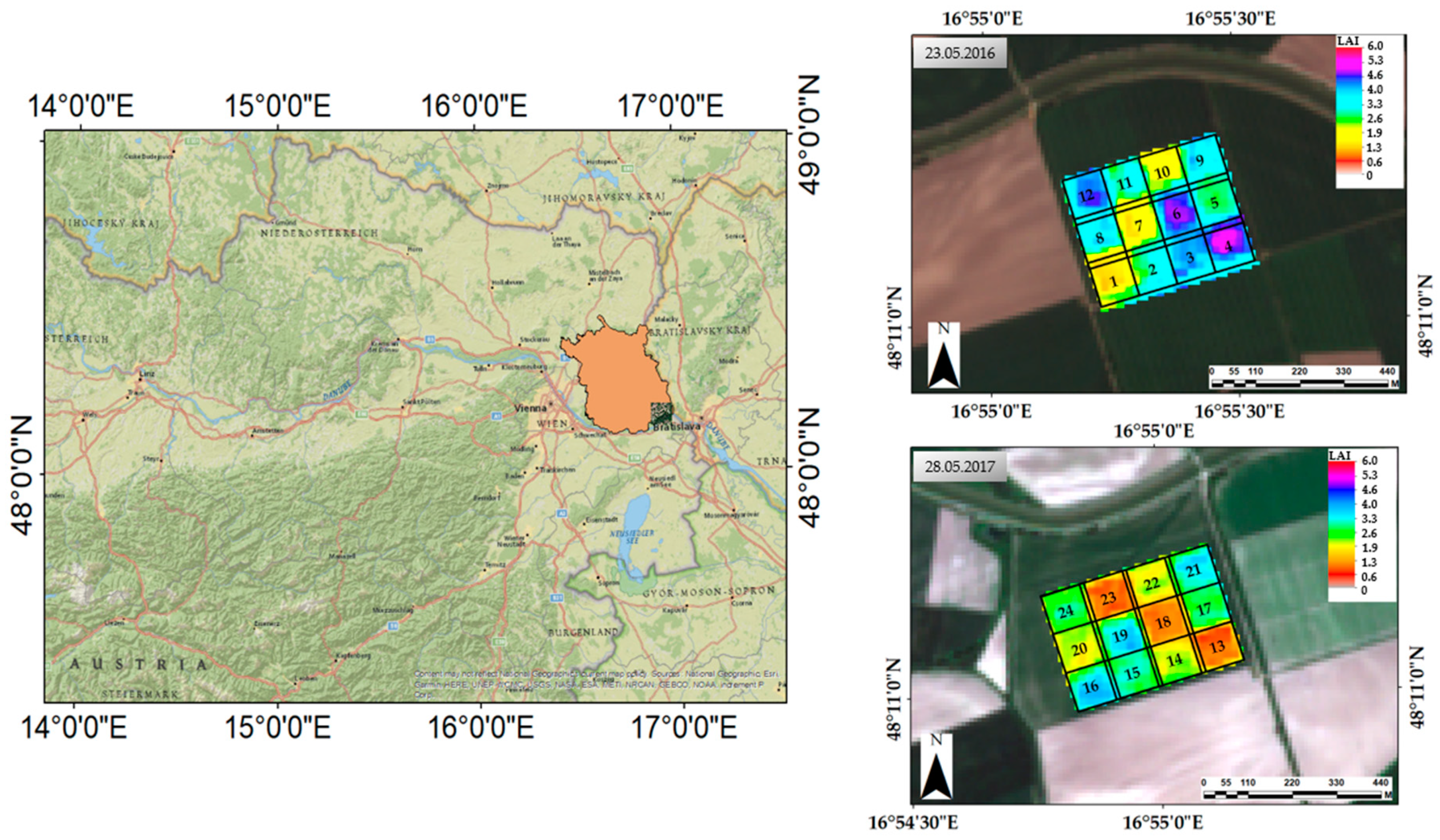
2.1. Study Area
2.2. Experimental Plots
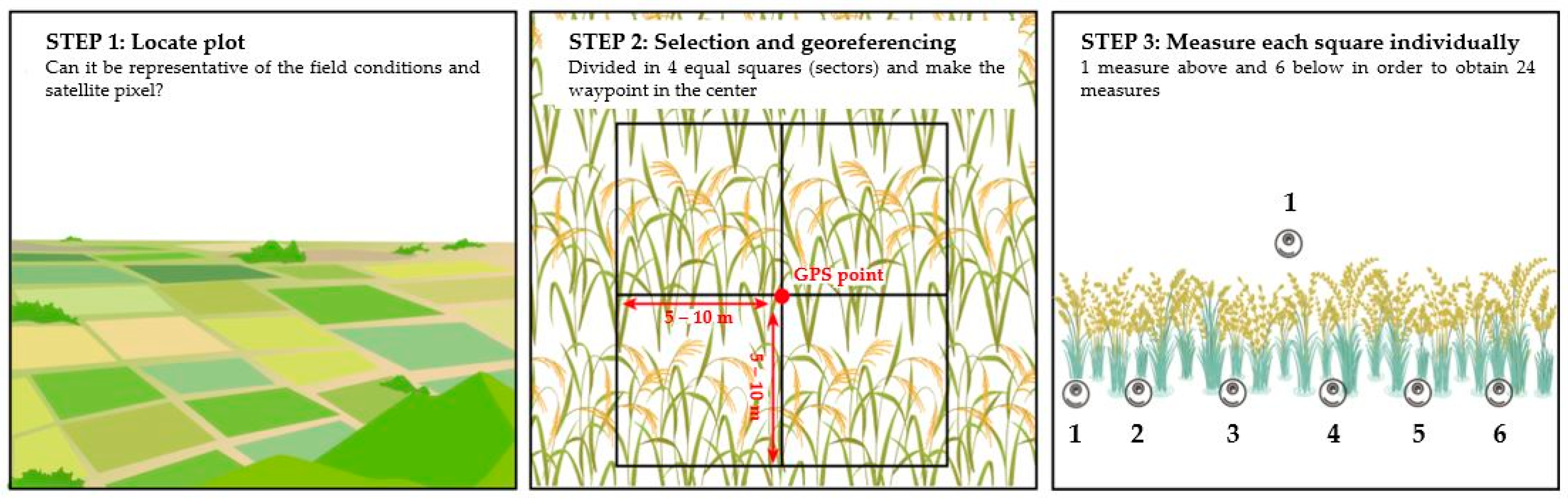
2.3. Leaf Area Index Measurements
2.4. Satellite Data
Leaf Area Index
2.5. EPIC Input and Forcing
2.5.1. EPIC Model
2.5.2. EPIC Input Data
2.5.3. Model Calibration
2.5.4. Data Assimilation
2.6. Accuracy Assessment
3. Results
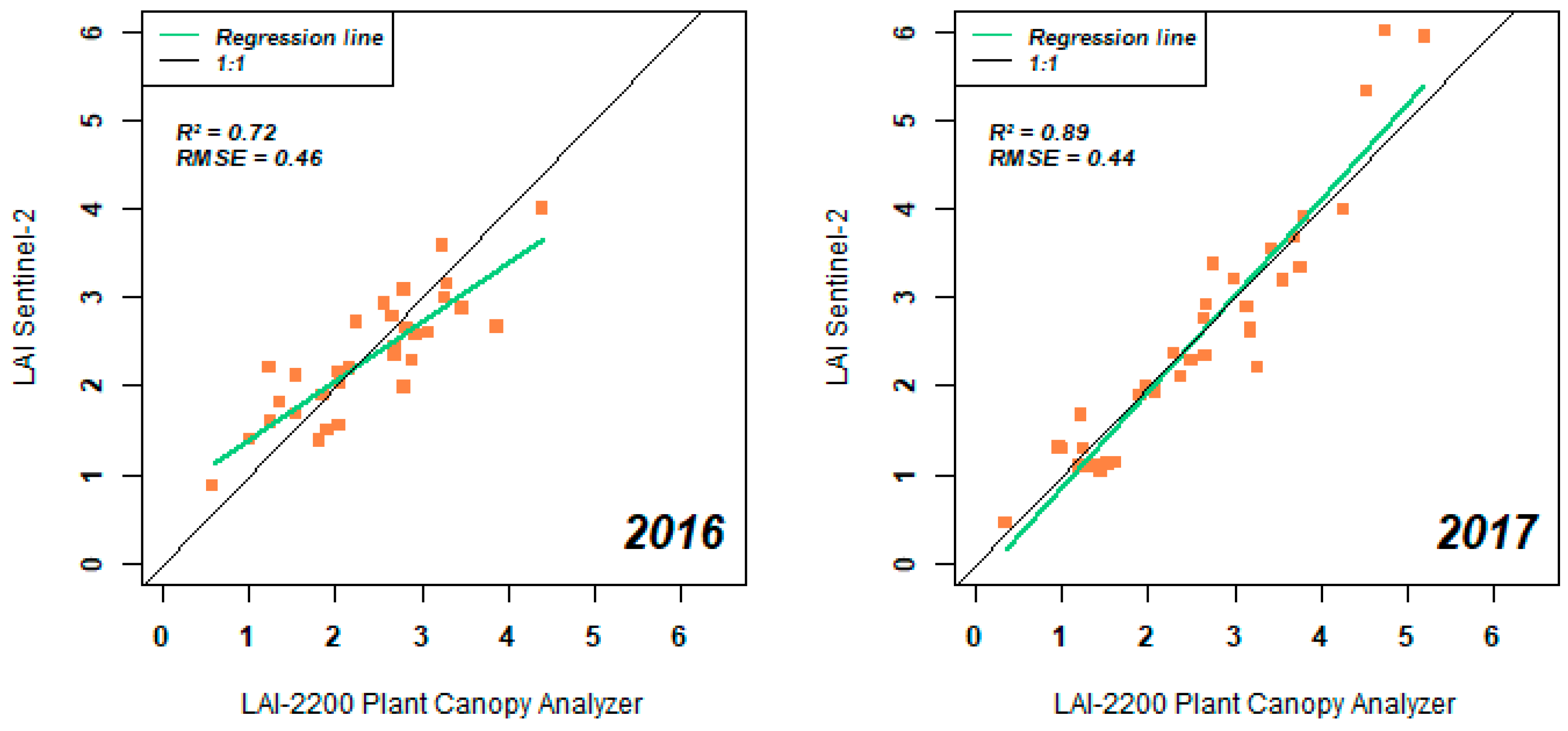
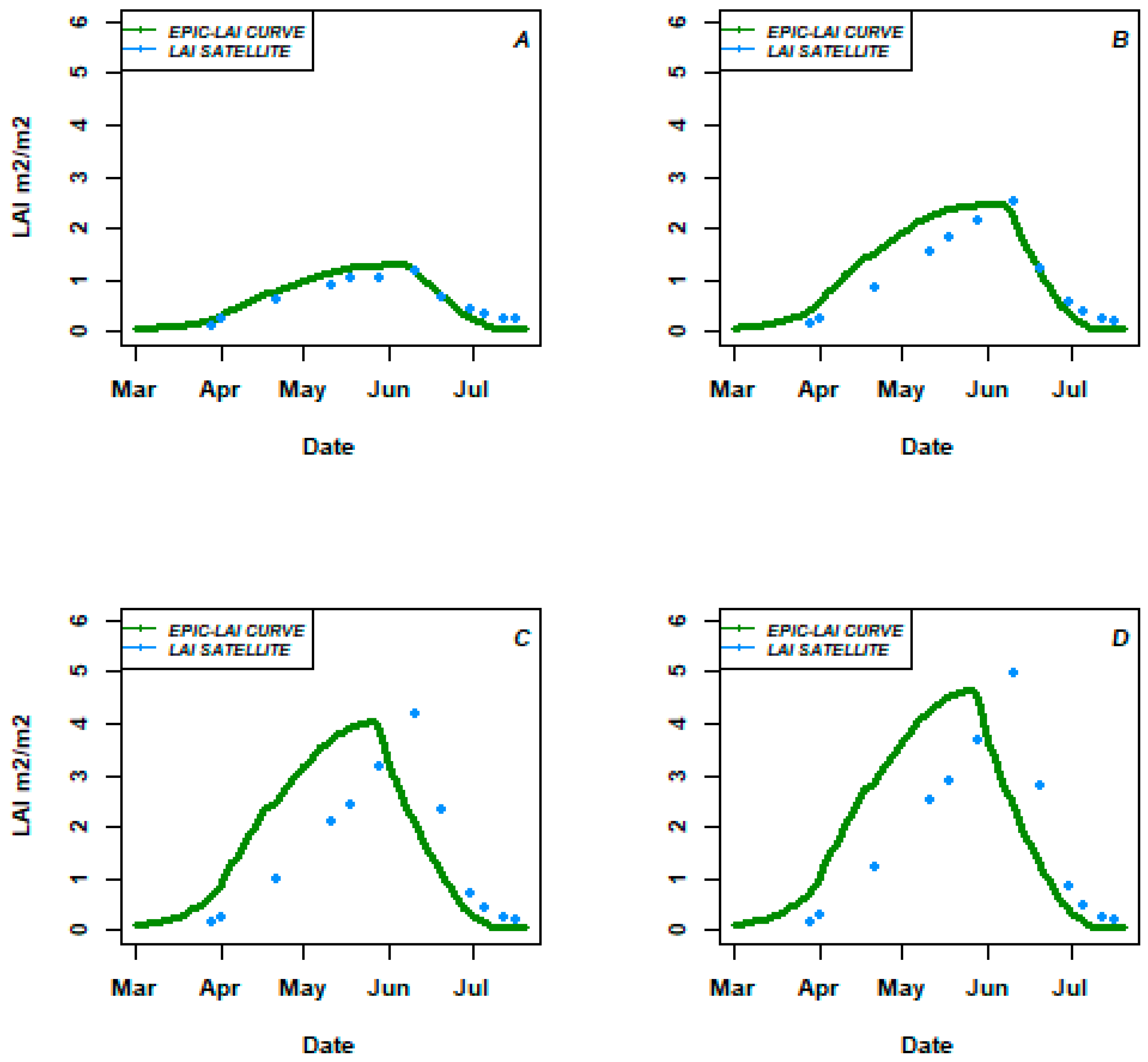
3.1. LAI Validation
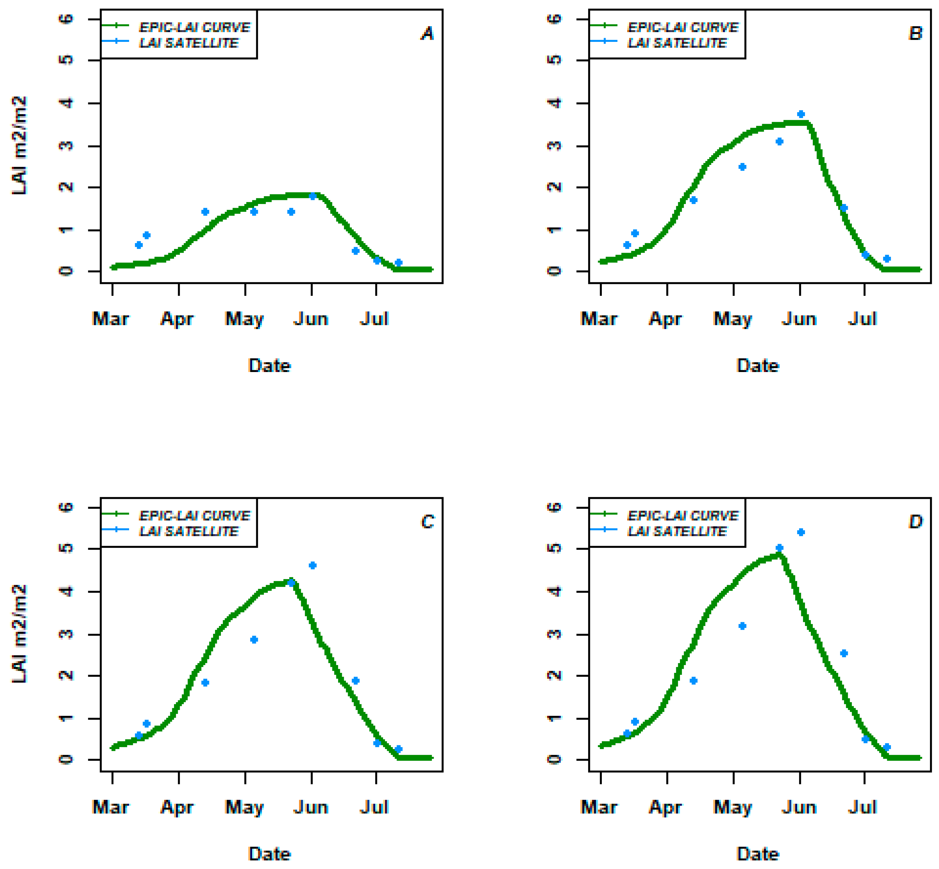
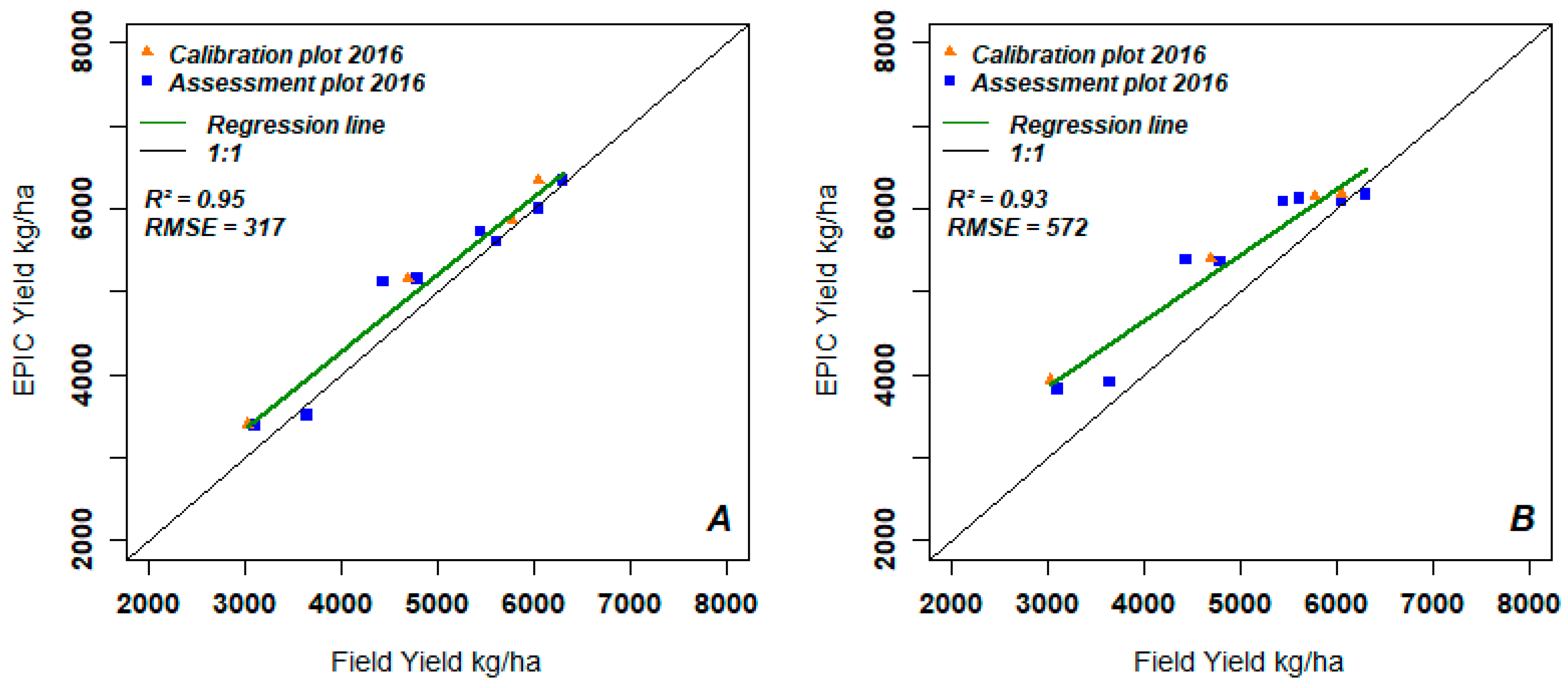
3.2. EPIC Calibration and Assessment
3.3. Yield Estimation in 2016
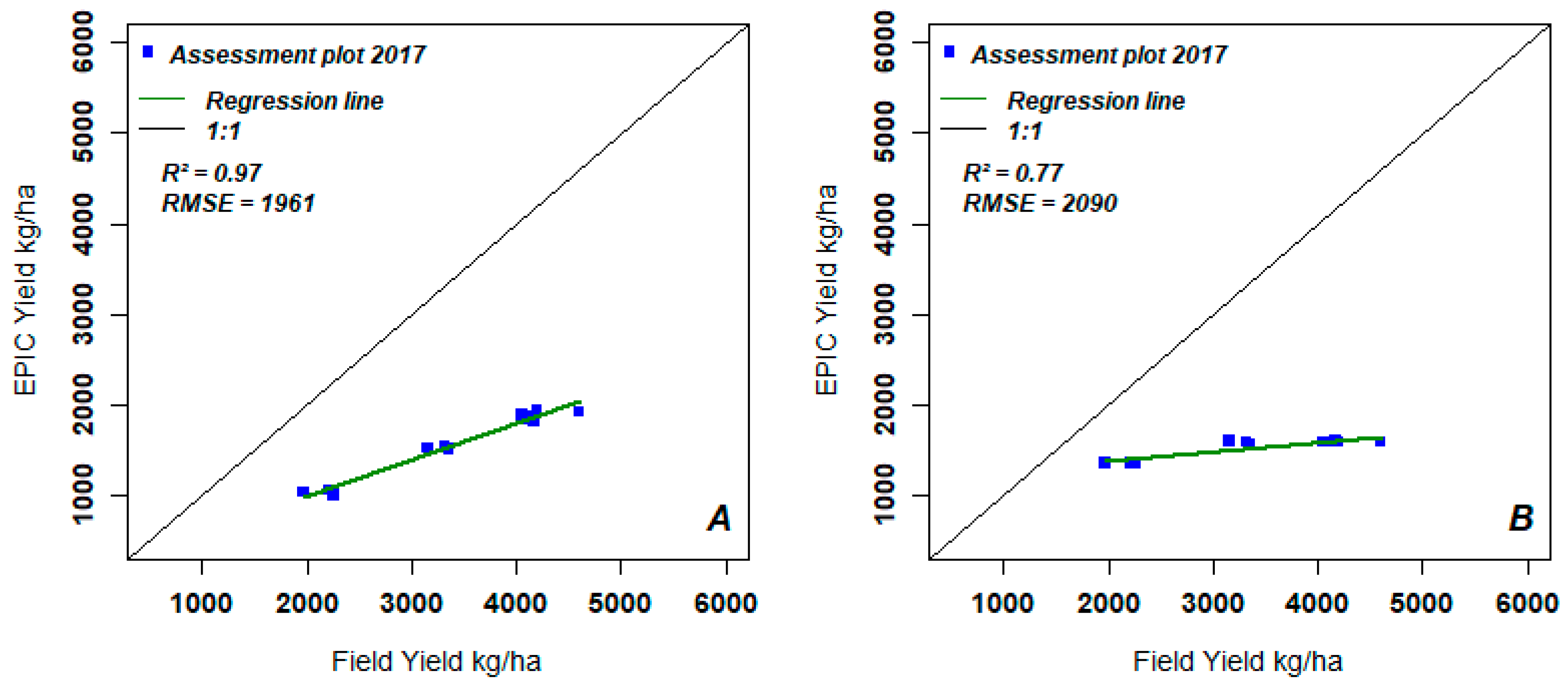
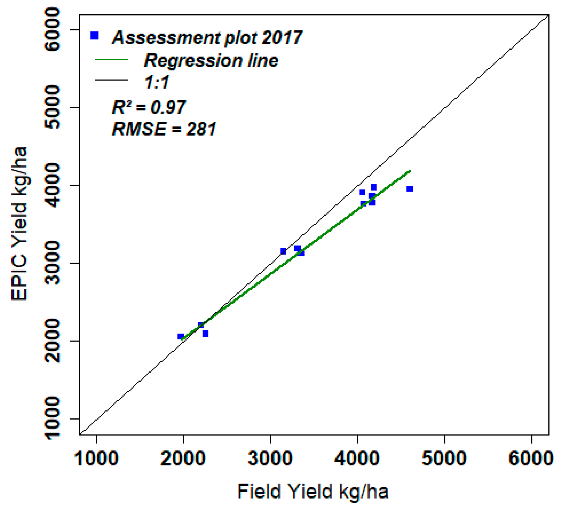
3.4. Yield Estimation for 2017
4. Discussion
5. Conclusions
Author Contributions
Funding
Acknowledgments
Conflicts of Interest
References
- Mueller, N.D.; Gerber, J.S.; Johnston, M.; Ray, D.K.; Ramankutty, N.; Foley, J.A. Closing yield gaps through nutrient and water management. Nature 2012, 490, 254–257. [Google Scholar] [CrossRef]
- Battude, M.; Al Bitar, A.; Morin, D.; Cros, J.; Huc, M.; Marais Sicre, C.; Le Dantec, V.; Demarez, V. Estimating maize biomass and yield over large areas using high spatial and temporal resolution Sentinel-2 like remote sensing data. Remote Sens. Environ. 2016, 184, 668–681. [Google Scholar] [CrossRef]
- Yuan, W.; Chen, Y.; Xia, J.; Dong, W.; Magliulo, V.; Moors, E.; Olesen, J.E.; Zhang, H. Estimating crop yield using a satellite-based light use efficiency model. Ecol. Indic. 2015, 60, 702–709. [Google Scholar] [CrossRef]
- Atzberger, C. Advances in remote sensing of agriculture: Context description, existing operational monitoring systems and major information needs. Remote Sens. 2013, 5, 949–981. [Google Scholar] [CrossRef]
- Wall, L.; Larocque, D.; Léger, P.M. The early explanatory power of NDVI in crop yield modelling. Int. J. Remote Sens. 2008, 29, 2211–2225. [Google Scholar] [CrossRef]
- Rembold, F.; Atzberger, C.; Savin, I.; Rojas, O. Using low resolution satellite imagery for yield prediction and yield anomaly detection. Remote Sens. 2013, 5, 1704–1733. [Google Scholar] [CrossRef]
- Manjunath, K.R.; Potdar, M.B.; Purohit, N.L. Large area operational wheat yield model development and validation based on spectral and meteorological data. Int. J. Remote Sens. 2002, 23, 3023–3038. [Google Scholar] [CrossRef]
- Balaghi, R.; Tychon, B.; Eerens, H.; Jlibene, M. Empirical regression models using NDVI, rainfall and temperature data for the early prediction of wheat grain yields in Morocco. Int. J. Appl. Earth Obs. Geoinf. 2008, 10, 438–452. [Google Scholar] [CrossRef] [Green Version]
- Monteith, J.L.; Moss, C.J. Climate and the Efficiency of Crop Production in Britain [and Discussion]. Philos. Trans. R. Soc. B Biol. Sci. 2006, 281, 277–294. [Google Scholar] [CrossRef]
- Moulin, S.; Bondeau, A.; Delecolle, R. Combining agricultural crop models and satellite observations: From field to regional scales. Int. J. Remote Sens. 1998, 19, 1021–1036. [Google Scholar] [CrossRef]
- Huang, Y.; Zhu, Y.; Li, W.; Cao, W.; Tian, Y. Assimilating Remotely Sensed Information with the WheatGrow Model Based on the Ensemble Square Root Filter For improving Regional Wheat Yield Forecasts. Plant Prod. Sci. 2013, 16, 352–364. [Google Scholar] [CrossRef]
- Launay, M.; Guerif, M. Assimilating remote sensing data into a crop model to improve predictive performance for spatial applications. Agric. Ecosyst. Environ. 2005, 111, 321–339. [Google Scholar] [CrossRef]
- Gowda, P.T.; Satyareddi, S.A.; Manjunath, S. Crop Growth Modeling: A Review. Res. Rev. J. Agric. Allied Sci. Crop. 2013, 2, 1–11. [Google Scholar]
- Kasampalis, D.; Alexandridis, T.; Deva, C.; Challinor, A.; Moshou, D.; Zalidis, G. Contribution of Remote Sensing on Crop Models: A Review. J. Imaging 2018, 4, 52. [Google Scholar] [CrossRef]
- Prevot, L.; Chauki, H.; Troufleau, D.; Weiss, M.; Baret, F.; Brisson, N. Assimilating optical and radar data into the STICS crop model for wheat. Agronomie 2003, 23, 297–303. [Google Scholar] [CrossRef] [Green Version]
- de Wit, A.J.W.; van Diepen, C.A. Crop model data assimilation with the Ensemble Kalman filter for improving regional crop yield forecasts. Agric. For. Meteorol. 2007, 146, 38–56. [Google Scholar] [CrossRef]
- Jin, X.; Kumar, L.; Li, Z.; Yang, G.; Wang, J. Review article A review of data assimilation of remote sensing and crop models. Eur. J. Agron. 2018, 92, 141–152. [Google Scholar] [CrossRef]
- Dorigo, W.A.; Zurita-milla, R.; De Wit, A.J.W.; Brazile, J. A review on reflective remote sensing and data assimilation techniques for enhanced agroecosystem modeling. Int. J. Appl. Earth Obs. Geoinf. 2007, 9, 165–193. [Google Scholar] [CrossRef]
- Machwitz, M.; Giustarini, L.; Bossung, C.; Frantz, D.; Schlerf, M.; Lilienthal, H.; Wandera, L.; Matgen, P.; Hoffmann, L.; Udelhoven, T. Enhanced biomass prediction by assimilating satellite data into a crop growth model. Environ. Model. Softw. 2014, 62, 437–453. [Google Scholar] [CrossRef]
- Fang, H.; Liang, S.; Hoogenboom, G.; Teasdale, J.; Cavigelli, M. Corn-yield estimation through assimilation of remotely sensed data into the CSM-CERES-Maize model. Int. J. Remote Sens. 2008, 29, 3011–3032. [Google Scholar] [CrossRef]
- Ma, G.; Huang, J.; Wu, W.; Fan, J.; Zou, J.; Wu, S. Assimilation of MODIS-LAI into the WOFOST model for forecasting regional winter wheat yield. Math. Comput. Model. 2013, 58, 634–643. [Google Scholar] [CrossRef]
- Ren, J.; Yu, F.; Qin, J.; Chen, Z.; Tang, H. Integrating remotely sensed LAI with EPIC model based on global optimization algorithm for regional crop yield assessment. In Proceedings of the IEEE International Geoscience and Remote Sensing Symposium, Honolulu, HI, USA, 25–30 July 2010. [Google Scholar]
- Tan, G.; Shibasaki, R. Global estimation of crop productivity and the impacts of global warming by GIS and EPIC integration. Ecol. Model. 2003, 168, 357–370. [Google Scholar] [CrossRef]
- Liu, J.; Chen, Z.; Sun, L.; Ren, J.; Jiang, Z.; Chen, J.; Li, H.; Li, Z. Application of Crop Model Data Assimilation with a Particle Filter for Estimating Regional Winter Wheat Yields. IEEE J. Sel. Top. Appl. Earth Obs. Remote Sens. 2014, 7, 4422–4431. [Google Scholar]
- Dente, L.; Satalino, G.; Mattia, F.; Rinaldi, M. Assimilation of leaf area index derived from ASAR and MERIS data into CERES-Wheat model to map wheat yield. Remote Sens. Environ. 2008, 112, 1395–1407. [Google Scholar] [CrossRef]
- Baret, F.; Buis, S. Estimating Canopy Characteristics from Remote Sensing Observations: Review of Methods and Associated Problems. In Advances in Land Remote Sensing; Springer: Dordrecht, The Netherlands, 2008; pp. 173–201. [Google Scholar]
- European Space Agency (ESA). SENTINEL-2 User Handbook; ESA: Paris, France, 2015; pp. 1–64.
- Richter, K.; Atzberger, C.; Vuolo, F.; Weihs, P.; Urso, G.D. Experimental assessment of the Sentinel-2 band setting for RTM-based LAI retrieval of sugar beet and maize. Can. J. Remote Sens. 2009, 35, 230–247. [Google Scholar] [CrossRef]
- Vuolo, F.; Zóltak, M.; Pipitone, C.; Zappa, L.; Wenng, H.; Immitzer, M.; Weiss, M.; Baret, F.; Atzberger, C. Data service platform for Sentinel-2 surface reflectance and value-added products: System use and examples. Remote Sens. 2016, 8, 938. [Google Scholar] [CrossRef]
- Upreti, D.; Huang, W.; Kong, W.; Pascucci, S.; Pignatti, S.; Zhou, X.; Ye, H.; Casa, R. A Comparison of Hybrid Machine Learning Algorithms for the Retrieval of Wheat Biophysical Variables from Sentinel-2. Remote Sens. 2019, 11, 481. [Google Scholar] [CrossRef]
- Vuolo, F.; Essl, L.; Zappa, L.; Sandén, T.; Spiegel, H. Water and nutrient management: The Austria case study of the FATIMA H2020 project. Adv. Anim. Biosci. 2017, 8, 400–405. [Google Scholar] [CrossRef]
- Fatima-H2020. Marchfeld Pilot Area in Austria. Available online: http://fatima-h2020.eu/pilots/austria-marchfeld/ (accessed on 14 January 2019).
- Thaler, S.; Eitzinger, J.; Trnka, M.; Dubrovsky, M. Impacts of climate change and alternative adaptation options on winter wheat yield and water productivity in a dry climate in Central Europe. J. Agric. Sci. 2012, 150, 537–555. [Google Scholar] [CrossRef]
- Vuolo, F.; Neugebauer, N.; Bolognesi, S.F.; Atzberger, C.; D’Urso, G. Estimation of leaf area index using DEIMOS-1 data: Application and transferability of a semi-empirical relationship between two agricultural areas. Remote Sens. 2013, 5, 1274–1291. [Google Scholar] [CrossRef]
- USDA. Natural Resources Conservation Service Soil. Available online: https://www.nrcs.usda.gov/wps/portal/nrcs/detail/soils/ref/?cid=nrcs142p2_054253 (accessed on 7 May 2019).
- LI_COR. LAI-2200 Plant Canopy Analyzer Instruction Manual; LI-COR: Lincoln, Nebraska, 2017; p. 262. [Google Scholar]
- LI-COR Biosciences—Impacting Lives Through Science. Available online: https://www.licor.com/ (accessed on 7 May 2019).
- Vuolo, F.; Dash, J.; Curran, P.J.; Lajas, D.; Kwiatkowska, E. Methodologies and uncertainties in the use of the terrestrial chlorophyll index for the sentinel-3 mission. Remote Sens. 2012, 4, 1112–1133. [Google Scholar] [CrossRef]
- González-Sanpedro, M.C.; Le Toan, T.; Moreno, J.; Kergoat, L.; Rubio, E. Seasonal variations of leaf area index of agricultural fields retrieved from Landsat data. Remote Sens. Environ. 2008, 112, 810–824. [Google Scholar] [CrossRef] [Green Version]
- Nelson, D.; Wang, J. Introduction to artificial neural systems. Neurocomputing 2003, 4, 328–330. [Google Scholar] [CrossRef]
- Lek, S.; Guégan, J.F. Artificial neural networks as a tool in ecological modelling, an introduction. Ecol. Model. 1999, 120, 1–9. [Google Scholar] [CrossRef]
- Weiss, M.; Baret, F. Sentinel2 ToolBox Level2 Products S2ToolBox Level 2 Products: LAI, FAPAR, FCOVER Version 1.1; INRA-CSE: Avignon, France, 2016; p. 53. [Google Scholar]
- Müller-Wilm, U. Sen2Cor Configuration and User Manual—Ref. S2-PDGS-MPC-L2A-SUM-V2.5.5; Telespazio VEGA: Luton, Bedfordshire, UK, 2018; p. 54. [Google Scholar]
- Williams, J.R.; Jones, C.A.; Kiniry, J.R.; Spanel, D.A. The EPIC Crop Growth Model. Trans. ASAE 1989, 32, 0497–0511. [Google Scholar] [CrossRef]
- Williams, J.R.; Dagitz, S.; Magre, M.; Meinardus, A.; Staglich, E.; Taylor, R. Environmental Policy Integrated Climate Model; Model User Manual Version 0810; Blackland Research and Extension Center A&M AgriLife: College Station, TX, USA, 2015. [Google Scholar]
- Kiniry, J.R.; Williams, J.R.; Major, D.J.; Izaurralde, R.C.; Gassman, P.W.; Morrison, M.; Bergentine, R.; Zentner, R.P. EPIC model parameters for cereal, oilseed, and forage crops in the northern Great Plains region. Can. J. Plant Sci. 2011, 75, 679–688. [Google Scholar] [CrossRef]
- Huang, M.; Gallichand, J.; Dang, T.; Shao, M. An evaluation of EPIC soil water and yield components in the gully region of Loess Plateau, China. J. Agric. Sci. 2006, 144, 339–348. [Google Scholar] [CrossRef]
- EPIC & APEX Model. Model Executables. Available online: https://epicapex.tamu.edu/model-executables/ (accessed on 9 October 2018).
- Constrained Nonlinear Optimization Algorithms. MATLAB & Simulink. Available online: https://ch.mathworks.com/help/optim/ug/constrained-nonlinear-optimization-algorithms.html#brnpd5f (accessed on 9 November 2018).
- Byrd, R.H.; Hribar, M.E.; Nocedal, J. An interior point method for large scale nonlinear programming. SIAM J. Optim. 1999, 9, 877–900. [Google Scholar] [CrossRef]
- Backhaus, K.; Erichson, B.; Weiber, R. Fortgeschrittene Multivariate Analysemethoden eine Anwendungsorientierte Einführung; Springer-Lehrbuch: Basel, Switzerland, 2013. [Google Scholar]
- Soliani, L. Fondamenti di Statistica Applicata All’analisi e Alla Gestione Dell’ambiente. 2001. Available online: https://dokumen.tips/documents/fondamenti-di-statistica-applicata-allanalisi-ambientalepdf25-distribuzioni.html (accessed on 7 May 2019).
- Richter, K.; Atzberger, C.; Hank, T.B.; Mauser, W. Derivation of biophysical variables from Earth observation data: Validation and statistical measures. J. Appl. Remote Sens. 2012, 6, 063557. [Google Scholar] [CrossRef]
- Bellocchi, G.; Rivington, M.; Donatelli, M.; Matthews, K. Validation of biophysical models: Issues and methodologies. Agron. Sustain. Dev. 2010, 30, 109–130. [Google Scholar] [CrossRef]
- Vanino, S.; Nino, P.; De Michele, C.; Falanga Bolognesi, S.; D’Urso, G.; Di Bene, C.; Pennelli, B.; Vuolo, F.; Farina, R.; Pulighe, G. Capability of Sentinel-2 data for estimating maximum evapotranspiration and irrigation requirements for tomato crop in Central Italy. Remote Sens. Environ. 2018, 215, 452–470. [Google Scholar] [CrossRef]
- Wang, H.; Zhu, Y.; Li, W.; Cao, W.; Tian, Y. Integrating remotely sensed leaf area index and leaf nitrogen accumulation with RiceGrow model based on particle swarm optimization algorithm for rice grain yield assessment. J. Appl. Remote Sens. 2014, 8, 083674. [Google Scholar] [CrossRef] [Green Version]
- Lazauskas, S.; Povilaitis, V.; Antanaitis, Š.; Sakalauskaite, J.; Sakalauskiene, S.; Pšibišauskiene, G.; Auškalniene, O.; Raudonius, S.; Duchovskis, P. Winter wheat leaf area index under low and moderate input management and climate change. J. Food Agric. Environ. 2012, 10, 588–593. [Google Scholar]
- Balkovič, J.; van der Velde, M.; Schmid, E.; Skalský, R.; Khabarov, N.; Obersteiner, M.; Stürmer, B.; Xiong, W. Pan-European crop modelling with EPIC: Implementation, up-scaling and regional crop yield validation. Agric. Syst. 2013, 120, 61–75. [Google Scholar] [CrossRef]


| S2 Acquisition Date | Cloud Cover | LAI Ground Measurements Date | |
|---|---|---|---|
| 2016 | April 13 | 0.0% | April 13–18 1 |
| April 26 | 18.4% | April 25 | |
| May 06 | 3.8% | May 02–09 | |
| 2017 | April 21 | 10.3% | April 25 |
| May 18 | 51.9% | May 18 | |
| May 28 | 0.0% | May 23–29 | |
| June 20 | 0.0% | June 19 |
| S2 Acquisition Date | Cloud Cover | S2 Acquisition Date | Cloud Cover | ||
|---|---|---|---|---|---|
| 2016 | March 14 | 1.3% | 2017 | March 29 | 11.7% |
| March 17 | 3.7% | April 1 | 0.0% | ||
| April 13 | 0.0% | April 21 | 10.3% | ||
| May 6 | 3.8% | May 11 | 79.3% | ||
| May 23 | 35.6% | May 18 | 52% | ||
| June 2 | 31.8% | May 28 | 0.0% | ||
| June 22 | 4.9% | June 10 | 43% | ||
| July 2 | 0.0% | June 20 | 0.0% | ||
| July 12 | 4.0% | June 30 | 29.6% | ||
| July 5 | 7.7% | ||||
| July 12 | 14.8% | ||||
| July 17 | 12% |
© 2019 by the authors. Licensee MDPI, Basel, Switzerland. This article is an open access article distributed under the terms and conditions of the Creative Commons Attribution (CC BY) license (http://creativecommons.org/licenses/by/4.0/).
Share and Cite
Novelli, F.; Spiegel, H.; Sandén, T.; Vuolo, F. Assimilation of Sentinel-2 Leaf Area Index Data into a Physically-Based Crop Growth Model for Yield Estimation. Agronomy 2019, 9, 255. https://0-doi-org.brum.beds.ac.uk/10.3390/agronomy9050255
Novelli F, Spiegel H, Sandén T, Vuolo F. Assimilation of Sentinel-2 Leaf Area Index Data into a Physically-Based Crop Growth Model for Yield Estimation. Agronomy. 2019; 9(5):255. https://0-doi-org.brum.beds.ac.uk/10.3390/agronomy9050255
Chicago/Turabian StyleNovelli, Francesco, Heide Spiegel, Taru Sandén, and Francesco Vuolo. 2019. "Assimilation of Sentinel-2 Leaf Area Index Data into a Physically-Based Crop Growth Model for Yield Estimation" Agronomy 9, no. 5: 255. https://0-doi-org.brum.beds.ac.uk/10.3390/agronomy9050255