Modelling Crop Transpiration in Greenhouses: Different Models for Different Applications


1
Department of Agriculture Crop Production and Rural Environment, University of Thessaly, 38446 Volos, Greece
2
Greenhouse Horticulture, Wageningen University & Research, 6708 PB Wageningen, The Netherlands
*
Author to whom correspondence should be addressed.
Agronomy 2019, 9(7), 392; https://0-doi-org.brum.beds.ac.uk/10.3390/agronomy9070392
Submission received: 9 June 2019
/
Revised: 12 July 2019
/
Accepted: 13 July 2019
/
Published: 17 July 2019
(This article belongs to the Special Issue Crop Evapotranspiration)
Abstract
:Models for the evapotranspiration of greenhouse crops are needed both for accurate irrigation and for the simulation or management of the greenhouse climate. For this purpose, several evapotranspiration models have been developed and presented, all based on the Penman–Monteith approach, the “big-leaf” model. So, on the one hand, relatively simple models have been developed for irrigation scheduling purposes, and on the other, “knowledge–mechanistic” models have been developed for climate control purposes. These models differ in the amount of detail about variables, such as stomatal and aerodynamic conductance. The aim of this review paper is to present the variables and parameters affecting greenhouse crop transpiration, and to analyze and discuss the existing models for its simulation. The common sub-models used for the simulation of crop transpiration in greenhouses (aerodynamic and stomatal conductances, and intercepted radiation) are evaluated. The worth of the multilayer models for the simulation of the mass and energy exchanges between crops and air are also analyzed and discussed. Following the presentation of the different models and approaches, it is obvious that the different applications for which these models have been developed entail varying requirements to the models, so that they cannot always be compared. Models developed in different locations (high–low latitudes or for closed or highly ventilated greenhouses) are discussed, and their sensitivity to different parameters is presented.
1. Introduction
Greenhouse cultivation is widely applied around the world, and today, it is estimated that about 405,000 ha [1] are cultivated under different types of permanent structures, in addition to about one million ha “solar greenhouses” in China, on which not many statistics are available. Cultivation under cover has several advantages, among which the possibility to control the climate conditions and increase the water use efficiency (WUE) are included. WUE under cover is reported to be from 3 to 10 times higher than under open field conditions [2,3]. Studying evapotranspiration may help to understand and improve the environment of plants, not only under greenhouse cultivation conditions, but also in open fields. The climate under cover and the water use efficiency are highly affected by the evapotranspiration (ET) under cover.
As referred in the literature [4], the modelling of transpiration is an aid to climate management, something that explains why several ET models have been developed and presented for the accurate irrigation of greenhouse crops and the simulation or management of the greenhouse climate under different greenhouse types and climate conditions. Each type of greenhouse provides a different microclimate, which in turn affects the physical process, including the transpiration of a greenhouse canopy. Estimations on how much energy is absorbed by the plant depends a lot on the greenhouse characteristics (cladding material), and on the ability of the climate control equipment (if present) to automatically modify/control the relevant climate factors. With the expansion of greenhouse culture all over the world, this has led to various models for ET estimation [4,5,6,7,8]. Thus, this work aims to review and discuss the available literature on the available ET models, their basic differences, and their use under different greenhouse climate conditions.
2. The Most Common Approaches
2.1. The Penman–Monteith Model
Evaporation (from soil) and transpiration (from the crop stomata) occur simultaneously, and there is no easy way of distinguishing between the two processes [5]. However, in many cases under greenhouse conditions, the soil is covered by a mulch that may considerably reduce the evaporation [9]. In the case of a non-mulched cropped soil, the evaporation is mainly determined by the water availability at the soil surface and the part of solar radiation reaching the soil surface. The solar irradiance reaching the soil is reduced during the growing period, as the plants develop and their canopy shades an increasing fraction of the ground area. When the crop is small, water is mainly lost by soil evaporation, but once plants are well developed and completely cover the soil, transpiration becomes the main process.
Crop transpiration in greenhouses could be estimated based on the crop energy balance [10] or on the mass transfer theory (also called as direct method), which links transpiration to leaf-to-air vapor pressure difference (e.g., [6,11,12,13], as shown below:
where λ (J kg−1) is the latent heat of vaporization, ET (kg m−2 s−1) is the evapotranspiration rate, γ (kPa K−1) is the psychrometric constant, ρ (kg m−3) and Cp (J kg−1 K−1) are the density and specific heat of air, respectively, Rn (W m−2) is the net radiation intercepted by the crop, gt (m s−1) is the total canopy conductance to water vapor transfer, Dc (kPa) is the canopy-to-air vapor pressure difference, and Hc (W m−2) is the sensible heat exchanged between the canopy and the air.
Energy balance: λET = Rn − Hc
The methods presented above may seem simple to use, but both require knowing the crop temperature (in order to calculate Hc or Dc), a measure that, although increasingly cheap and reliable, is not always available. It was in 1948, when Penman [14] combined the energy balance with the mass transfer theory and presented an equation to estimate the evaporation from an open water surface from standard climatological data of temperature, humidity, wind speed, and sunshine. This so-called combination method was further developed by many researchers and extended to cropped surfaces by introducing resistance factors, and the hypothesis that transpiration happens from a surface that is saturated at its temperature was formed. The Penman–Monteith (P–M) formula of the combination equation is as follows [15]:
where Di (kPa) denotes the vapor pressure deficit of the air, Δ denotes the slope of the saturation vapor pressure temperature relationship (kPa K−1), and rs and ra are the (bulk) crop stomatal and aerodynamic resistances, respectively (s m−1, and gc and ga are the crop stomatal and aerodynamic conductances, m s−1, respectively).
The application of the P–M formula requires knowledge of the variables that are not easily available. In principle, the aerodynamic and stomatal bulk conductances have to be known for each crop species and, possibly, for each cultivar. The aerodynamic conductance depends on the air velocity around and within the crop canopy, while the crop stomatal conductance is influenced by the climate and the water availability. Here, it is important to distinguish the following: when water supply is non-limiting, we speak about potential evapotranspiration. Therefore, for a model of potential evaporation, knowledge about water availability is not needed. Nevertheless, aerodynamic and stomatal conductances (even with non-limiting water supply) differ from one crop to another, and diverse varieties can be affected in a different way.
The limit for λET as ga → 0, known as the equilibrium evaporation (λETeq), is given by Equation (3a), and depends only on the available radiative energy, as follows:
The limit for λET as ga → ∞, known as imposed evaporation (λETimp), is given by Equation (3b), as follows:
The aerodynamic term λETimp is predominant when the crop surface is “coupled” to the ambient weather conditions, as the crop is exposed to strong wind and low radiation, while decoupling prevails when a well-watered canopy is exposed to bright sunshine, humid air, and a light wind, something that is usually the case for most greenhouse crops.
As the crop aerodynamic conductance in greenhouses may be much lower than that of an open field crop, greenhouse crops are usually strongly decoupled from the greenhouse atmosphere. Furthermore, greenhouse crops are also decoupled from the outside atmosphere because of the presence of the cover, and the heat and water released at the crop surface accumulate inside the greenhouse. Consequently, the transpiration rate adjusts until it reaches a stable equilibrium transpiration rate, dictated by the net radiation received, and the “permeability” of the cover for water vapor. However, this is not always the case for Mediterranean or similar warm conditions, where the transpiration rate is much more dependent on convection. In such conditions with higher ventilation rates than those observed for higher latitudes, the ventilation and the turbulent mixing are vigorous, the saturation deficit at the leaf surface is closely coupled to the deficit of ambient air, and the latter is directly influenced by the outdoor saturation deficit.
2.2. Simplified Models
As noted above, the use of the complete P–M formula requires knowledge of several variables that are not easily available. That is why researchers have tried to overcome the estimation of them by using a simplified λET formulae.
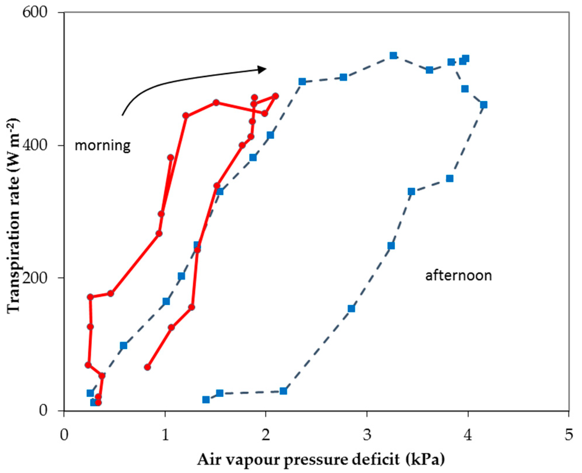
However, the models that do not consider all of the variables of the complete P–M formula implicitly assume a correlation between any two/three of them. For instance, the authors of [16,17,18] proposed a linear relationship with sun radiation alone, whereas the authors of [19,20] also included the energy input by the heating system of Dutch greenhouses. This approach may be simpler, but then the models include constants, which make the model empirical rather than mechanistic. In fact, for greenhouse conditions (usually supplied with plenty of water), many authors (e.g., [16,17,19] for tomato crop, [7] for cucumber crop, and [8] for rose crop), have reported a strong correlation between crop transpiration and solar radiation exists. Apparently, based on similar results, the author of [4] stated the following: “... it is an acknowledged fact that for most climates, transpiration can be better estimated as a function of measured radiation fluxes than of saturation deficit...”. The authors of [21] suggested that “the aerodynamic term could be eliminated from evapotranspiration prediction formulae for greenhouse conditions”, and argued that the two P–M terms are well correlated, because greenhouses, unlike the open field, are poorly ventilated, and, therefore, greenhouse crops are effectively “decoupled” from greenhouse air. However, the inter-correlation of greenhouse microclimate variables may be the case for rudimentary equipped greenhouses, where there are no means of greenhouse climate control other than natural ventilation, but it may not stand for greenhouses where control actions like heating, forced ventilation, cooling, or dehumidification are taken [22,23]. Figure 1 shows the correlation between the transpiration rate of a soilless rose crop and the air vapor pressure deficit (VPD) in a glasshouse cooled by natural ventilation or by a fog system, as presented by the authors of [24].
The authors of [24] showed that misting significantly changed the relation between λET and air VPD. It was shown that, as misting does not affect the solar radiation entering the greenhouse, the correlation between solar radiation and VPD is strongly affected by the system. Thus, it could be concluded that the presence of a climate control system that modifies the greenhouse microclimate parameters may change the degree of their correlation to crop transpiration.
For well-watered greenhouse crops, the simplest empirical formula used for λE prediction is based on a linear correlation between λET and solar radiation (Rs in W m−2) [16,18], of the following form:
where Kc is the crop coefficient depending on the crop development stage, and Aο and Bo are the coefficients determined by statistical adjustment. This relation, which is mainly valid at daily or weekly time scales, presents several drawbacks, as follows [23]:
λET = Ao Kc Rs + Bo
(i) A large amount of empiricism and inaccuracy in the determination of the crop coefficient Kc.
(ii) The vapor pressure deficit is not explicitly taken into account. Only in the case of a significant correlation between Rs and VPD, can Equation (4) give a satisfactory estimation of λET.
(iii) Equation (4) assigns a constant value (Bo) to nocturnal evapotranspiration, which can rise to a significant level in the case of heated greenhouses during cold periods [20]. In fact, the coefficient Bo averages in some way the influence of nocturnal heating, but cannot predict the effect of single climate variables on nocturnal values of λET.
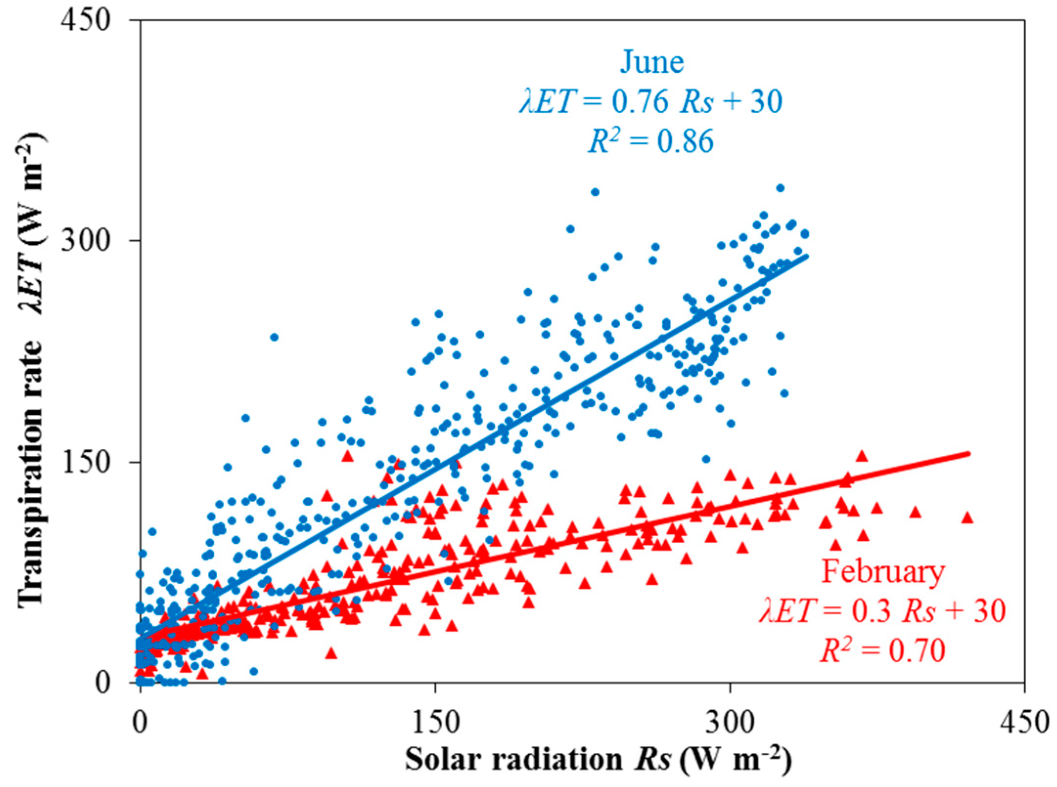
Furthermore, in addition to (ii), Equation (4) assumes a constant correlation between stomatal and aerodynamic conductance, something that is not always true, especially when different greenhouse climate control systems are used. For example, the relationship between the solar radiation and crop transpiration rate of a rose crop with the same leaf area index during two different seasons, winter and summer, is presented in Figure 2 [25]. In both cases, a linear relationship of λET = a Rs + b was obtained, with different values for the slope between the two cases. This effect may be partially explained by the differences in vapor pressure deficit, and in the stomatal and aerodynamic conductances observed during the two periods, as compared to the summer period, during winter, the greenhouse ventilation needs are very low. It has to be noted that the summer period measurements presented in Figure 2 were observed under shading, and that for the same value of incoming solar radiation during the two periods, a much higher value (two or three times higher) of air vapor pressure deficit was observed during summer than during winter. However, as solar radiation and vapor pressure deficit are correlated in rudimentarily equipped greenhouses, the effect of vapor pressure deficit on the crop transpiration rate was taken into account through the (radiation-related) slope of the above equation. The offset (b) is significant in both cases, and reflects the contribution of nocturnal evapotranspiration.
Nevertheless, Equation (4) is successfully applied in most irrigation controllers in high-tech greenhouses, which give a pre-set amount of water anytime a pre-set radiation is cumulated. Whenever cultivation is on substrate drain water, it is collected daily and its amount is used to calibrate the relationship.
Several improvements of this simple formula have been proposed. For instance, the authors of [23] suggested explicitly taking into account the influence of the VPD and leaf area index, and derived the following relationship from the formalism of Equation (2):
where, A (dimensionless) and B (W m−2 kPa−1) implicitly account for the following:
λET = A Rs + B Di
The first term of Equation (5) is known as the “radiation term”, and the second one as the “aerodynamic term” (sometimes called the “advection term”). Hence, A and B may be referred to as the “radiation coefficient” and the “aerodynamic coefficient”, respectively. The influence of radiation on A and B (via gc) may be disregarded for high-radiation levels, and the expected increase with the ventilation rate, through its effect on ga, is also ignored, based on previous studies [23,26], analysis [27], and experience [28]. Usually, coefficients A and B are estimated by the multilinear regression of the measured evapotranspiration against measured solar radiation and VPD. A and B are usually treated as constants for a given crop, or as simple functions of readily measurable quantities, such as the leaf area index (LAI). Thus, the authors of [23] suggested the following formulas for A and B as a functions of LAI:
where k is the extinction coefficient (see Section 2.4.3), and
A = a f1(LAI) = a [1-exp(-k LAI)]
B = b f2(LAI) = b LAI
In Equation (7b), LAI is considered as a multiplicative factor in the “advective” term of the Penman–Monteith equation. However, the authors of [29] noted that this may result in an overestimation for mature crops, where, in general, a large proportion of the leaves are shaded, less ventilated, and less active, and suggested modelling B in analogy with the modelling of A as follows:
where low LAI values (or low k) produce the same results as Equation (7b), as suggested by the authors of [23].
B = b f2(LAI) = (b/k) [1-exp(-k LAI)]
A and B have been identified for several greenhouse species, and have been presented by the authors of [29,30] (Table 2 of [29] and Table 6 of [30]). The divergence among and within the crops could be ascribed to differences in plant habit, stomatal resistance, and growing conditions. As noted by the authors of [30], in spite of scatter, there is an apparent negative correlation between A and B, with a significant R2. According to the authors of [31], two reasons may account for negative correlation between A and B, namely:
(i) a difference in greenhouse temperature. As Δ increases with temperature, the first and the second term of Equation (2) (A and B, respectively, as shown in Equation (6)) are functions of the temperature, if gc and ga do not change; however, A increases with temperature, while B decreases when the temperature increases.
(ii) The decoupling of the greenhouse from the atmospheric air is a result of poor ventilation, as previously discussed.
Most of the literature where the advective term is not used for the estimation of λET originates from Central and North Europe, where the greenhouse ventilation needs are low, and thus greenhouse crops are decoupled from the internal and external atmosphere. In this case, changes in the radiation load may significantly affect crop transpiration, as the radiative part constitutes the major part of crop transpiration. This is not the case in coupled greenhouse crops (mainly the Mediterranean [32]), where changes of air VPD and air velocity (e.g., by means of cooling systems) may be as important as changes in radiation loads in order to affect crop transpiration, and in this case, the advective part of crop transpiration is also important. The advective contribution represents 43% of the total transpiration for a May–June greenhouse tomato crop in the South of France [33], and both radiative and advective components of transpiration must be considered in the models [34,35].
2.3. Single and Multilayer Models
It is a fact that the combination equation and all of its simplified versions represent the crop as a single layer, with one temperature and one transpiration rate. One may wonder whether scaling up from leaf to canopy would make it necessary to take into account the structure and distribution of the crop leaves and their parameters and the distribution of the microclimate parameters at each “group of leaves”. However, this is not an easy task, as a canopy is an irregular bunch of leaves at different layers, with different properties, and exposed to different conditions, something that is very complicate to describe by simple-realistic models. That is why the calculation and simulation of mass and energy exchanges between crop and air are dominated by two main trends [36].
The first assumes that the crop is divided into discrete layers, and the exchange calculations require knowledge and a description of the conditions in each crop layer [11]. Simple sub-models are used for calculating the exchange at each layer, but sophisticated models or measurements are required for calculating the required unknown variables for each layer (temperature, humidity, radiation, and air velocity), and incorporate the individual layers into a comprehensive model (crop level).
The second trend to calculate the mass and energy exchanges between crop and air assumes that the crop is a large leaf, and that all internal layers are located in the same climatic conditions [37]. The approach is the so-called “big-leaf model”, because it specifies the stand-atmosphere exchange in terms of a crop aerodynamic resistance (ga) analogous to the boundary layer resistance around a single leaf (gl,a), and canopy resistance (gc), which corresponds to the stomatal conductance (gl,s) of a leaf. The methods for estimating ga and gc are described in Section 2.4.
According to the above definitions, the P–M equation can be applied to both approaches, but, while in the multilayer approach the model integrates the fluxes from each layer to give the total flux; in the big-leaf approach, the properties of the whole canopy are integrated (not necessarily averaged) onto a single leaf/layer, and then the model is used to calculate the flux. As is noted by the authors of [38], the determination of the boundary and stomatal resistances is the most important barrier for the accuracy and usefulness of multilayer models, which is analogous to that for single-layer models.
The net radiation, and the bulk stomatal and aerodynamic resistances must be specified a priori in a single-layer model, while layer-by-layer values of the radiation and the individual-leaf resistances are needed in a multilayer model [38]. The authors of [7] note that for microclimate control purposes at the canopy level, it may be necessary to consider the different layers of the crop, as there might be high temperature, stomatal conductance, and transpiration rate differences between the different crop layers. Furthermore, the author of [11] noted that under the big leaf assumption, the averaging processes of the climate parameters in the greenhouse canopies may produce a mean air temperature or velocity within the canopy, which may be significantly different from that above the canopy [39,40,41]. In the case that large temperature differences do exist between the microclimate at the level of the crop and above the crop, the big leaf approach may introduce some errors into the estimation of the stomatal and aerodynamic conductances. That is why the author of [8] mentioned that under greenhouse conditions, the microclimate variables experience large spatial variations [42] that make the big leaf approach scaling-up from leaf to canopy difficult to justify.
Indeed, as the authors of [38] noted, “single-layer models are appropriate when the scale of study is much larger than that of the vegetation itself while multilayer models are appropriate when it is necessary to resolve detail within the canopy, either because the detail is important in its own right or because the height scale of the vegetation is comparable to that of the system under study”. The latter would be the case of a greenhouse. However, the authors of [33] compared a single-layer model and a multi-layer model, and showed that the two models gave similar values of crop transpiration rates. Similar results were also presented by the authors of [43], who compared the results obtained by single- and two-layer approach models for crop transpiration estimations. They noted that the two-layer method was more accurate in terms of the latent heat flux estimation than the one-layer approach. However, they did not find statistically significant differences between the one- and two-layer approaches, and concluded that it probably would not be relevant to multiply sensors inside the greenhouse in order to obtain only a small improvement in the transpiration estimate. Indeed, the authors of [44] showed that crop transpiration in two greenhouse compartments, where opposite gradients of air properties were artificially created, was within 95% of each other. Their explanation was that the contribution of the available energy (sun radiation) was overwhelming the relatively small effect of air properties.
As the authors of [38] write, “A correct model is one which not only gives acceptably precise predictions but does so for sound physical reasons, while a useful model is one which is modest enough in its data and computational requirements to be worth the trouble of using”. So, the authors of [38] mention that “since both the single-layer and multilayer models are based on the physical principles of combined energy and diffusion control of evaporation, both models are correct”. However, both are based on the values of aerodynamic and stomatal conductance, which are not always easy to find.
2.4. The Sub-Models
Concerning λET modelling in greenhouses, as observed by the authors of [29], most of the models proposed are of the type of Equation (5), λET = A Rs + B Di, which is derived from the Penman–Monteith equation, and employs the big leaf approach. However, there are differences in the type of the sub-models used to estimate the stomatal and aerodynamic conductances, and in how the radiation part (solar or net) is modelled. In the following part of this section, an attempt is made to present, compare, and discuss the different sub-models used and the assumptions considered.
2.4.1. Aerodynamic Conductance
The aerodynamic conductance, which regulates the transfer of heat and water from the surface of the leaf to the ambient air, can be calculated by the classical theory of heat transfer using dimensionless numbers [4]. Following the non-dimensional heat transfer theory [45,46,47], the boundary layer conductance to the heat transfer (gb, m s-1) from bodies of different shapes can be expressed as a function of the dimensionless Nusselt number (Nu), as follows:
where κ (m2 s−1) is the thermal diffusivity of air, and d (m) is the characteristic dimension of the body. The characteristic dimension of a leaf can be calculated as a function of its length and width dimensions [48]. Depending on the prevailing heat transfer mechanism (forced or free convection, that is, wind speed or temperature difference), Nu is expressed as a function either of the Reynolds number (Re), as follows:
where u is air velocity (m s−1), and ν is the kinematic viscosity of the air (m2 s−1),
or the Grashoff number (Gr) [46], as follows:
where g is the gravitational acceleration (m s−2), β is the coefficient of the volumetric expansion of air (K−1), and ΔT (K) is the temperature difference between the leaf and its environment. The parameters n and m depend, in both cases, on the type of air flow (laminar or turbulent) and other characteristics of the system. They are tabulated in Table A5 of the literature [46].
Re = u d/ν → Nu = n Rem
The heat transfer mode in terms of free, mixed, or forced convention in calculating the boundary layer conductance depends on the relative magnitude of the Gr and Re numbers. It is indicated [4] that for Gr/Re2 >15, the convention mode could be considered free, while for Gr/Re2 <0.1, the convection could be considered forced. Unfortunately, for most greenhouse conditions, the convection is in between these two limits, and then is considered as mixed [4,11,35,49,50,51,52].
Many semi-empirical models have been proposed, mirroring the variety of systems we have in greenhouses. The author of [53], for instance, proposed the following correlation for the boundary layer conductance of a rose crop in a non-ventilated greenhouse:
which proves the prevalence of free convection in the absence of ventilation, where Ti and Tc (in °C) indicate the air and crop temperature, respectively, and d is the “typical dimension” of the leaves/leaflets. The author of [4] proposed a general formula with the vectoral sum of free (vertical) and forced (horizontal) convection.
gb = 1.9 [(Ti − Tc)/d]0.25
Its units (m or cm) should be the same as that used for the wind speed, u (m/s or cm/s). For tomato, it was determined that d ≈ 0.05 m. The authors of [54] observed that, given that turbulence within the greenhouse canopies seldom is the product of canopy-to-air temperature difference alone, the sign of this difference is unlikely to play a big role in determining the efficiency of the heat exchange.
The problem that usually arises from the use of the above equations is associated with the choice of the points at which the temperature difference and the air velocity are considered. There are many disagreements in the literature as to what temperature difference should be taken. The author of [11] mentions that if the aerodynamic conductance is calculated from measurements of air temperature from above and not within the crop, the result is more of an indicative value. Nevertheless, as the authors of [55] showed, besides the well-known thermal feed-back (which ensures that crop transpiration is not very sensitive to the aerodynamic resistance), the hydraulic feed-back in greenhouses further depresses the sensitivity of the transpiration of greenhouse crops to variations (or inaccurate estimates) of the aerodynamic resistance.
Using the big leaf approach, the canopy aerodynamic conductance (ga) can be considered, in a first approximation, as the product of the leaf boundary layer conductance and crop leaf area index (LAI), multiplied by a factor of two, accounting for the fact that there are two surfaces of each leaf exchanging heat with the air, as follows:
ga = 2 LAI gb,l
2.4.2. Stomatal Conductance
The author of [56] advanced the hypothesis that that the complex stomatal behavior we know has been shaped by selection towards maximal transpiration efficiency (that is, maximal carbon intake per unit of water lost). Although this does explain the known trend of stomatal behavior with respect to climate variables, such as radiation, vapor pressure deficit, or carbon dioxide concentration, we still do not have an explanatory model of stomatal behavior.
The most complete relationship, which reflects the influence of environmental factors on the behavior of stomata, is that of the authors of [57], as follows:
where CO2 indicates the CO2 concentration in the air. In this relationship, stomatal conductance is expressed as a function of maximum conductance (gM), multiplied by a number of reducing factors. These factors are independent of each other, impose crop water stress, and their result is multiplied and not added to calculate the final result. Several forms and parameters of the functions f1, f2, f3, and f4 have been proposed for greenhouse crops (e.g., [4,22,23,34,35]), while the value of maximum conductance (gM), which varies from species to species, can be measured or found in the literature. In any case, from the above factors affecting stomatal conductance, there is little doubt that the most important role is played by radiation, and thus the other factors are often ignored or indirectly taken into account through their correlation with solar radiation. The authors of [58] concluded that the air temperature and CO2 influences on stomatal conductance are not significant, and do not need to be included in a tomato transpiration model. Anyhow, given the high correlation between air temperature and vapor deficit in natural conditions, usually, accounting for one of the two would suffice. Even worse, accounting for both may result in large overestimates of the resistance (and underestimates of transpiration) under a high VPD (f.i., [48]). In addition, the authors of [59] have advanced doubts about the functional dependence of the stomatal resistance and vapor deficit. The mathematical functions f1, f2, f3, and f4, and their constant coefficients for different crops found in the literature, are given in Table 1.
gc = gM f1(Rn) f2(Di) f3(Ti) f4(CO2)
Following Equation (18) and using the big leaf approach, the canopy stomatal conductance (ga) can be considered as a function of the leaf stomatal layer conductance and the crop leaf area index (LAI), as follows:
gc = 2 LAI gs,l
Vapor loss from the two surfaces of a leaf is not the same, as the stomata density is usually much higher on the lower surface of the leaves. However, Equation (15) defines stomatal conductance in a way that allows for its experimental determination, whereas accounting for dis-uniformity between the two surfaces would unnecessarily complicate things. Therefore, this representation is the one that is preferred in the literature.
2.4.3. Net Radiation of a Greenhouse Crop
The standard method for determining the net radiation of field crops is by placing a net radiometer (measures the difference between the downward and upward radiation of all wavelengths) far above the crop, and one (or more) meter(s) for the heat flux into the soil. Then, one can state that the amount of radiation absorbed by the crop is the difference between what is measured by the net radiometer and the soil flux meter. This would not work in a greenhouse—there may be an energy source (the heating system) between the two meters, besides the obvious limitation to having a net radiometer “far enough” from the crop. So, the approach required for greenhouse crops is to determine the net amount of radiation (both short- and long-wave) that is really absorbed by the crop.
Usually, the analogy first introduced by the authors of [60] is applied, which simulates the canopy as a “turbid medium”, the LAI having the function of the thickness (d) of the medium. Then, a fraction, 1-e-ksLAI, of the incident shortwave radiation is absorbed, and the longwave (thermal) radiation is exchanged by a “big leaf” with the shape of the horizontal projection of all of the leaves, which is called the “soil cover”, 1-e-klLAI, with ks and kl being the extinction coefficients for short- and long-wave radiation, respectively.
Indeed, this radiation transfer model is also implicitly applied in most versions of simplified models (see Equation (7a)). The authors of [61] demonstrated that k depends on the distribution of the inclination angles of the leaves, and on their optical properties (reflection, absorption). As these are not the same for short- and longwave radiation, the extinction coefficient (which is, in fact defined by this model) will vary among crops (various leaf angles distribution), and depends on the waveband used to determine it.
As the range of temperatures in a greenhouse is rather limited, during the daytime, the net exchange of the thermal radiation is often neglected, and the net radiation of the crop is written as follows:
Rn = a(1-e-ksLAI) Rs
The coefficient (a) accounts for the fact that not all of the incoming radiation will be absorbed, even by a crop with a (very) large LAI—all leaves are reflecting some (green) light, and row crops will never reach full soil cover. The authors of [62] determined the coefficient (a) from the geometry of the rows, a representation adopted by the authors of [4]. For the typical geometry of a tall greenhouse crop, the authors of [63] proposed that a = 0.86 and ks = 0.7.
3. Transpiration from External Climate
It is a fact that humidity within a greenhouse is not a truly independent climate variable—it does depend on the transpiration of the crop within. That is, transpiration pushes vapor into the air, which, in turn, reduces transpiration. The strength of this “hydraulic feed-back” [64] is determined by the processes removing vapor from the air—ventilation and condensation. Therefore, in principle, greenhouse crop transpiration should be related to the conditions outside, through the processes coupling in- and out-side climate (ventilation and condensation on the greenhouse cover).
The authors of [55] have shown that the greenhouse vapor balance can be solved for the vapor concentration of the air, and that the equilibrium (steady conditions) vapor concentration of the air is as follows:
where the superscript * indicates “at saturation”, and the following is true: χeff (g m−3) is an “effective” vapor concentration of the leaves, which accounts for the effect of net radiation on leaf temperature; χr* (g m−3), the “effective” vapor concentration at the cover (the saturated vapor concentration at a cover temperature); χo (g m−3) vapor concentration of the air outside; gt (m s−1) canopy conductance on the transpiration flow; gcd (m s−1) the conductance for condensation; when the conditions do not lead to condensation, it is equal to 0; gv (m s−1) the conductance for ventilation (see Table 2 below for typical values).
The effective vapor concentration of the leaves (χeff) is defined by the following:
with χa* being the saturated vapor concentration at air temperature (which is a function exclusively of air temperature), and ε being the dimensionless ratio of the latent to sensible heat content of saturated air for a change of 1 °C in temperature.
The canopy conductance is defined as follows:
Substitution of Equations (17)–(19) in (1b) gives the crop transpiration in a greenhouse as function of outside conditions and the “coupling” between in- and out (ventilation, condensation):
However, this is of little practical use, as seldom are the condensation and ventilation rate known. Indeed, a transpiration model for greenhouse crops growing in a Mediterranean environment was proposed by the authors of [65], based on outdoor conditions. They compared their results with those obtained by the P–M model, and noted that it is clear that considering the outside climate instead of the inside climate as a boundary condition implies a deterioration of the transpiration model performances. However, they observed only a slight underestimation and loss of prediction of the model in May, while in March, the underestimation of the transpiration fluxes reached almost 20%. The model performed better during the day than during the night, and from March to May. The weakening of the model performances noticed in winter and night-time, that is, when a greenhouse is hardly ventilated, conforms to the observation [64] that the (negative) gain of the hydraulic feed-back loop is more important when the ventilation rate is small, and that it will tend to disappear if the greenhouse is well ventilated. That is, a greenhouse crop transpiration model is more likely to be accurate in a well-controlled and not much ventilated Dutch greenhouse, than in a low-tech, highly ventilated Mediterranean greenhouse.
An interesting consequence is that, as the feed-back dampens the effect of the stomatal regulation and of the boundary layer conductance on the transpiration of greenhouse crops, any inaccuracy in the estimate of both conductances will result in a relatively smaller inaccuracy of the estimate of transpiration.
4. Different Models for Different Applications
A general review of the models developed for the simulation of greenhouse crop transpiration was presented in the previous sections. It was shown that the (P–M) mechanistic approach explains the processes, and is at the basis of all of the models. When the purpose is determining water loss (thus irrigation water requirement), simplified models such as in [23,66], are perfectly suitable, whereas the P–M basis is explicit in “knowledge–mechanistic” models, such as in [4,34,65] models, which propose a sub-model for the stomatal and boundary layer resistances/conductances, and the net radiation of greenhouse crops.
The irrigation models are classes of models designed for action, and are based on a two-step approach, consisting of (i) a phase of identification of their parameters, and (ii) a phase of prediction. Note that these two phases may not use the same set of data, and that in order to predict the transpiration rate of a crop, you need first to measure it in order to calibrate the model. This class of models is also similar to the purely command models derived from the theory of control command, with closed-loop transfer functions based on linear or even nonlinear systems. In that case, one has only to determine the main driving forces behind transpiration, for example, saturation deficit and global solar or net radiation, and by measuring the input and output, one can identify the parameters.
On the other hand, the second class of models concerns “knowledge” models, where parameter identification is not necessary, because all of the knowledge that is needed for the computation of the output is concentrated into the formula and its attached parameters. Thus, in that case, only the phase of prediction exists, because the model’s parameters are supposed to be universal, and, combined with the formula, they are sufficient to capture the essential of the reality that one wants to describe. If one refers, for example, to the model by authors of [65], or to the original Stanghellini model [4], no identification phase is needed for these models, even for tuning the parameters for stomatal and aerodynamic conductances. That is why most of the parameters of the mechanistic models may have a better estimation accuracy.
Some studies compared the performance of the transpiration models under greenhouse conditions. The authors of [43] presented a comparison of the performance of the different models found in the literature [67,68,69,70], as shown in Table 3.
Without making a comparison among the models, recently, the authors of [71] showed that a “Stanghellini model”, whereby the stomatal resistance was solely a function of sun radiation, could very well predict the transpiration of a tomato crop in a naturally ventilated greenhouse in China.
Are All Sub-Models Equally Necessary?
So, it seems that P–M-based models are the most suited to estimating greenhouse crop transpiration rates on a time basis short enough for climate- rather than irrigation- management. However, the amount of (empirical) parameters needed for the required sub-models of aerodynamic and canopy resistance, as well as the net radiation of the crop, may be daunting. Therefore, one may wonder how accurate each sub-model needs to be.
As reported above, the authors of [64] already observed that in the case that the gain of the hydraulic feed-back loop increases (poorly ventilated, well insulated, that is, “decoupled” greenhouses), the “control” of both resistances on the transpiration process is lost. As far as the boundary layer resistance is concerned, this applies to nearly all conditions. Indeed, the sensitivity analysis of the authors of [71] confirmed that there is hardly any loss of accuracy when using a constant value (rather than a sub-model) for the boundary layer resistance, as done, for instance, by the authors of [26,44], provided a good average is correctly identified [64,70]. With respect to the stomatal resistance, this review leads us to agree with the conclusion by the authors of [64], that “the development of an accurate model… of the stomatal conductance…has turned out to be a superfluous sophistication”, provided that (a) the order of magnitude of the conductance with the stomata fully open, and (b) the behavior with respect to light, are correctly identified.
On the other hand, the “decoupled” conditions mentioned above, make it mandatory to make a correct estimate of the energy available for transpiration, which is the net radiation of the crop. This is true, whatever the purpose of the model; also, for simplified models dealing with rather long-term transpiration, the A coefficient of Equation (5) needs to be calibrated. Indeed, as we have seen, the coefficient is often modelled according to the “turbid medium” representation. At first sight, this bartering of one empirical coefficient with two does not make sense, were it not for the fact that we know more about the new two than the previous one, as they are linked to physical properties of the canopy that we are (more) able to identify. Nevertheless, as these properties change among crops (think of leaf inclination, row/no rows, etc.), whenever using published values, one should be aware of the conditions and the crops for which they were calibrated. As what is usually (if at all) measured is sun radiation outside the greenhouse, the transmissivity of the greenhouse is first and foremost.
5. Conclusions
Being at the forefront of “precision agriculture”, greenhouses increasingly need precision management of (fert)irrigation and climate. Knowledge of crop transpiration at relatively short time intervals (hours/minutes) is necessary in both cases. As the measurement of transpiration on that time scale (be it by weighing lysimeters or sap-flow measurement) is both cumbersome and expensive, it is common to rely on estimates/models of crop transpiration. We have shown that the Penman–Monteith approach, combining the physical processes of energy balance and mass and heat transfer, is at the basis of all models and estimates. What changes among them is the degree of “aggregation” of variables and the (empirical) parameters, which matches the accuracy required by the application. We have discussed the example of irrigation scheduling when drain measurement allows for the daily calibration of the ratio of water-use to radiation cumulated.
Whenever a high degree of accuracy (on a relatively short term) is required, the P–M method, including the most complete sub-models for crop net radiation, stomatal, and aerodynamic resistance [4] is found to perform best, although the difference with less complete models may be small/not significant. When looking for simplifications, a constant (but accurate) value for the aerodynamic resistance should be the first, and a simple (empirical) model relating stomatal resistance only to light would be the second. On the other hand, an accurate determination of the net radiation available to the crop is mandatory. This means that the sun radiation should be measured, and the parameters shaping its absorption by the crop should be accurately defined.
Author Contributions
N.K. and C.S. conceived and designed the contents of the manuscript; analyzed the available literature; and wrote the paper.
Funding
This research received no external funding.
Conflicts of Interest
The authors declare no conflict of interest.
References
- Abdessalam, O.A. Preface. In Good Agricultural Practices for Greenhouse Vegetable Crops: Principles for Mediterranean Climate Areas; FAO Plant Production and Protection Paper 217; Baudoin, W., Nono-Womdim, R., Lutaladio, N., Hodder, A., Castilla, N., Leonardi, C., De Pascale, S., Quaryouti, M., Eds.; FAO: Rome, Italy, 2013. [Google Scholar]
- Fernández, M.D.; Gallardo, M.; Bonachela, S.; Orgaz, F.; Thompson, R.B.; Fereres, E. Water use and production of a greenhouse pepper crop under optimum and limited water supply. J. Hortic. Sci. Biotechnol. 2005, 80, 87–96. [Google Scholar] [CrossRef]
- Stanghellini, C. Horticultural production in greenhouses: Efficient use of water. Acta Hortic. 2014, 1034, 25–32. [Google Scholar] [CrossRef]
- Stanghellini, C. Transpiration of Greenhouse Crops an Aid to Climate Management. Ph.D. Thesis, Wageningen University, Wageningen, The Netherlands, 1987. [Google Scholar]
- Allen, R.G.; Pereira, L.S.; Raes, D.; Smith, M. Crop evapotranspiration. In Guidelines for Computing Crop Water Requirements; FAO Irrigation and Drainage Paper 56; FAO: Rome, Italy, 1998. [Google Scholar]
- Kittas, C.; Katsoulas, N.; Baille, A. Transpiration and canopy resistance of greenhouse soilless roses in Greece. Measurements and modeling. Acta Hortic. 1999, 507, 61–68. [Google Scholar] [CrossRef]
- Yang, X.; Short, T.H.; Robert, D.F.; Bauerle, W.L. Transpiration, leaf temperature and stomatal resistance of a cucumber crop. Agric. For. Meteorol. 1990, 51, 197–209. [Google Scholar] [CrossRef]
- Katsoulas, N.; Kittas, C.; Baille, A. Estimating transpiration rate and canopy resistance of a rose crop in a fan-ventilated greenhouse. Acta Hortic. 1999, 548, 303–309. [Google Scholar] [CrossRef]
- Tarara, J.M. Microclimate modification with plastic mulch. HortScience 2000, 35, 169–180. [Google Scholar] [CrossRef]
- Seginer, I.; Kantz, D. In-situ determination of transfer coefficients for heat and water vapour in a small greenhouse. J. Agric. Eng. Res. 1986, 35, 39–54. [Google Scholar] [CrossRef]
- Yang, X. Comments on ‘Thermal and aerodynamic conditions in greenhouses in relation to estimation of heat flux and evapotranspiration’. Agric. For. Meteorol. 1995, 77, 131–136. [Google Scholar] [CrossRef]
- Leonardi, C.; Baille, A.; Guichard, S. Predicting transpiration of shaded and non-shaded tomato fruits under greenhouse environments. Sci. Hortic. 2000, 84, 297–307. [Google Scholar] [CrossRef]
- Boulard, T.; Fatnassi, H.; Roy, J.C.; Lagier, J.; Fargues, J.; Smits, N.; Rougier, M.; Jeannequin, B. Effect of greenhouse ventilation on humidity of inside air and in leaf boundary-layer. Agric. For. Meteorol. 2004, 125, 225–239. [Google Scholar] [CrossRef]
- Penman, H.L. Natural evaporation from open water, bare soil and grass. Proc. R. Soc. Lond. A 1948, 193, 120–145. [Google Scholar] [CrossRef] [Green Version]
- Monteith, J.L. Evaporation and environment. In Symposia of the Society for Experimental Biology; Cambridge University Press (CUP): Cambridge, UK, 1965; Volume 19, pp. 205–234. [Google Scholar]
- Morris, L.G.; Neale, F.E.; Postlethwaite, J.D. The transpiration of glasshouse crops and its relationship to the incoming solar radiation. J. Agric. Eng. Res. 1957, 2, 111–122. [Google Scholar]
- De Villèle, O. Besoins en eau des cultures sous serres—Essai de conduite des arrosages en fonction de l’ensoleillement. Acta Hortic. 1972, 35, 123–135. [Google Scholar]
- Stanhill, G.; Scholte Albers, J. Solar radiation and water loss from glasshouse roses. J. Amer. Soc. Hortic. Sci. 1974, 99, 107–110. [Google Scholar]
- Van der Post, C.J.; van Schie, J.J.; de Graaf, R. Energy balance and water supply in glasshouses in the West-Netherlands. Acta Hortic. 1974, 35, 13–22. [Google Scholar] [CrossRef]
- De Graaf, R. Influence of moisture deficit leaf-air and cultural practices on transpiration of glasshouse roses. Acta Hortic. 1995, 401, 545–552. [Google Scholar] [CrossRef]
- Jones, H.G.; Tardieu, F. Modelling water relations of horticultural crops: A review. Sci. Hortic. 1998, 74, 21–46. [Google Scholar] [CrossRef]
- Bakker, J.C. Leaf conductance of four glasshouse vegetable crops as affected by air humidity. Agric. For. Meteorol. 1991, 55, 23–36. [Google Scholar] [CrossRef]
- Baille, M.; Baille, A.; Delmon, D. Microclimate and transpiration of greenhouse rose crops. Agric. For. Meteorol. 1994, 71, 83–97. [Google Scholar] [CrossRef]
- Katsoulas, N.; Baille, A.; Kittas, C. Effect of air misting on transpiration and bulk conductances of a greenhouse rose canopy. Agric. For. Meteorol. 2001, 106, 233–247. [Google Scholar] [CrossRef]
- Kittas, C.; Katsoulas, N.; Tchamitchian, M. Greenhouse Soilless Rose Crop Transpiration. Application for Accurate Irrigation Control. In Proceedings of the VII Conference on Protection and Restoration of the Environment, Mykonos, Greece, 28 June–1 July 2004; pp. 998–1005. Available online: http://pre14.civil.auth.gr/index.php/previous-conferences/previous-conferences (accessed on 7 June 2019).
- Kittas, C.; Baille, A.; Katsoulas, N. Influence of misting on the diurnal hysteresis of canopy transpiration rate and conductance in a rose greenhouse. Acta Hortic. 1999, 534, 185–193. [Google Scholar] [CrossRef]
- Seginer, I. Transpirational cooling of a greenhouse crop with partial ground cover. Agric. For. Meteorol. 1994, 71, 265–281. [Google Scholar] [CrossRef]
- Seginer, I.; Tarnopolsky, M. Response of plants to ventilation regimes. In Transpirational Cooling of Greenhouse Crops; Chapter T3, Final Report, BARD Project IS-2538-95R; Seginer, I., Willits, D.H., Raviv, M., Peet, M.M., Eds.; Agricultural Research Organization of Israel: Bet Dagan, Israel, 2000; pp. 165–171. [Google Scholar]
- Seginer, I. Alternative design formulae for the ventilation rate of greenhouses. J. Agric. Eng. Res. 1997, 68, 355–365. [Google Scholar] [CrossRef]
- Carmassi, G.; Bacci, L.; Bronzini, M.; Incrocci, L.; Maggini, R.; Bellocchi, G.; Massa, D.; Pardossi, A. Modelling transpiration of greenhouse gerbera (Gerbera jamesonii H. Bolus) grown in substrate with saline water in a Mediterranean climate. Sci. Hortic. 2013, 156, 9–18. [Google Scholar] [CrossRef]
- Seginer, I. The Penman–Monteith Evapotranspiration Equation as an Element in Greenhouse Ventilation Design. Biosyst. Eng. 2002, 82, 423–439. [Google Scholar] [CrossRef]
- Katsoulas, N.; Sapounas, A.; de Zwart, F.; Dieleman, J.A.; Stanghellini, C. Reducing ventilation requirements in semi-closed greenhouses increases water use efficiency. Agric. Water. Man. 2015, 156, 90–99. [Google Scholar] [CrossRef]
- Jemaa, R. Mise AU Point ET Validation de Modèles DE Transpiration de Cultures de Tomate Hors SOL Sous Serre. Application à La Conduite DE La Fert-Irrigation. Ph.D. Thesis, Brittany National College of Architecture, Rennes, France, 1995; p. 111. [Google Scholar]
- Boulard, T.; Baille, A.; Le Gall, F. Etude de différentes méthodes de refroidissement sur le climat et la transpiration de tomates de serre. Agronomie 1991, 11, 543–554. [Google Scholar] [CrossRef]
- Papadakis, G.; Frangoudakis, A.; Kyritsis, S. Experimental investigation and modelling of heat mass transfer between a tomato crop and greenhouse environment. J. Agric. Eng. Res. 1994, 57, 217–227. [Google Scholar] [CrossRef]
- González-Real, M.M. Estudio y Modelizacion de Intercambios Gaseosos en Cultivos de Rosas Bajo Invernadero. Ph.D. Τhesis, Universidad Politecnica de Valencia, Valencia, Spain, 1995; p. 192. [Google Scholar]
- Stanghellini, C. Response to comments on ‘Thermal and aerodynamic conditions in greenhouses in relation to estimation of heat flux and evapotranspiration’. Agric. For. Meteorol. 1995, 77, 137–138. [Google Scholar] [CrossRef]
- Raupach, M.R.; Finnigan, J.J. Single-layer models of evaporation from plant canopies are incorrect but useful, whereas mutlilayer models are correct but useless: Discuss. Aust. J. Plant Physiol. 1988, 15, 705–716. [Google Scholar]
- Yang, X.; Short, T.H.; Fox, R.D.; Bauerle, W.L. The microclimate and transpiration of a greenhouse cucumber crop. Am. Soc. Agric. Eng. 1989, 32, 2143–2150. [Google Scholar] [CrossRef]
- Kittas, C.; Katsoulas, N.; Baille, A. Influence of greenhouse ventilation regime on microclimate and energy partitioning of a rose canopy during summer conditions. J. Agric. Eng. Res. 2001, 79, 349–360. [Google Scholar] [CrossRef]
- Kittas, C.; Katsoulas, N.; Baille, A. Influence of an aluminised thermal screen on greenhouse microclimate and canopy energy balance. Trans. ASAE 2001, 46, 1653–1663. [Google Scholar] [CrossRef]
- Bojaca, C.R.; Gil, R.; Cooman, A. Use of geostatistical and crop growth modelling to assess the variability of greenhouse tomato yield caused by spatial temperature variations. Comp. Electr. Agric. 2009, 65, 219–227. [Google Scholar] [CrossRef]
- Morille, B.; Migeon, C.; Bournet, P. Is the Penman–Monteith model adapted to predict crop transpiration under greenhouse conditions? Application to a New Guinea Impatiens crop. Sci. Hortic. 2013, 152, 80–91. [Google Scholar] [CrossRef]
- Stanghellini, C.; Dieleman, J.A.; Driever, S.M.; Marcelis, L.F.M. Modelling the effect of the position of cooling elements on the vertical profile of transpiration in a greenhouse tomato crop. Acta Hortic. 2012, 952, 763–769. [Google Scholar] [CrossRef]
- Kreith, F. Principles of Heat Transfer, 3rd ed.; Intext Educational Publishers: New York, NY, USA, 1973; p. 656. [Google Scholar]
- Monteith, J.L.; Unsworth, M.H. Principles of Environmental Physics, 4th ed.; Academic Press: Cambridge, MA, USA, 2014; p. 401. [Google Scholar]
- Schuepp, P.H. Leaf boundary layers. New Phytol. 1993, 125, 477–507. [Google Scholar] [CrossRef]
- Montero, J.I.; Antón, A.; Muñoz, P.; Lorenzo, P. Transpiration from geranium grown under high temperatures and low humidities in greenhouses. Agric. For. Meteorol. 2001, 107, 323–332. [Google Scholar] [CrossRef]
- Katsoulas, N.; Baille, A.; Kittas, C. Leaf boundary layer conductance in ventilated greenhouses. An experimental approach. Agric. For. Meteorol. 2007, 144, 180–192. [Google Scholar] [CrossRef]
- Bailey, B.J.; Montero, J.I.; Biel, C.; Wilkinson, D.J.; Anton, A.; Jolliet, O. Transpiration of Ficus benjamina: Comparison of measurements with predictions of the Penman-Monteith model and a simplified version. Agric. For. Meteorol. 1993, 65, 229–243. [Google Scholar] [CrossRef]
- Kitano, M.; Eguchi, H. Buoyancy effect on forced convection in the leaf boundary layer. Plant Cell Env. 1990, 13, 965–970. [Google Scholar] [CrossRef]
- Zhang, L.; Lemeur, R. Effect of aerodynamic resistance on energy balance and Penman-Monteith estimates of evapotranspiration in greenhouse conditions. Agric. For. Meteorol. 1992, 58, 209–228. [Google Scholar] [CrossRef]
- Seginer, I. On the night transpiration of greenhouse roses under glass or plastic cover. Agric. For. Meteorol. 1984, 30, 257–268. [Google Scholar] [CrossRef]
- Stanghellini, C. Mixed convection above greenhouse crop canopies. Agric. For. Meteorol. 1993, 66, 111–117. [Google Scholar] [CrossRef]
- Stanghellini, C.; de Jong, T. A model of humidity and its applications in a greenhouse. Agric. For. Meteorol. 1995, 76, 129–148. [Google Scholar] [CrossRef]
- Cowan, I.R. Regulation of water use in relation to carbon gain in higher plants. In Physiological Plant Ecology II; Lange, O.L., Novel, P.S., Osmond, C.B., Zeigler, H., Eds.; Springer: Berlin, Germany, 1982; pp. 589–614. [Google Scholar]
- Jarvis, P.G. The interpretation of the variations in leaf water potential and stomatal conductance found in canopies in the field. Philos. Trans. R. Soc. Lond. B 1976, 273, 593–610. [Google Scholar] [CrossRef]
- Jolliet, O.; Bailey, B.J. The effect of climate on tomato transpiration in greenhouses: Measurements and models comparison. Agric. For. Meteorol. 1992, 58, 43–62. [Google Scholar] [CrossRef]
- Fuchs, M.; Stanghellini, C. The functional dependence of canopy conductance on water vapour pressure deficit revisited. Int. J. Biometeorol. 2018, 62, 1211–1220. [Google Scholar] [CrossRef]
- Monsi, M.; Saeki, T. Uber den Lichtfaktor in den Pflanzengesellschaften und seine Bedeutung für die Stoffproduktion. Jpn. J. Bot. 1953, 14, 22–25. [Google Scholar]
- Ross, J. Radiative transfer in plant communities. In Vegetation and the Atmosphere; Monteith, J.L., Ed.; Academic Press: London, UK, 1975; pp. 13–52. [Google Scholar]
- Goudriaan, J. Crop Micrometeorology: A Simulation Study, Simulation Monographs; Pudoc: Wageningen, The Netherlands, 1977; p. 249. [Google Scholar]
- Bontsema, J.; Hemming, J.; Stanghellini, C.; De Visser, P.; Van Henten, E.J.; Budding, J.; Rieswijk, T.; Nieboer, S. On-line estimation of the transpiration in greenhouse horticulture. In Proceedings of the Agricontrol 2007, 2nd IFAC International Conference on Modeling and Design of Control Systems in Agriculture, Osijek, Croatia, 3–5 September 2007; pp. 29–34. [Google Scholar]
- Aubinet, M.; Deltour, J.; de Halleux, D.; Nijskens, J. Stomatal regulation in greenhouse crops: Analysis and simulation. Agric. For. Meteorol. 1989, 48, 21–44. [Google Scholar] [CrossRef]
- Boulard, T.; Wang, S. Greenhouse crop transpiration simulation from external climate conditions. Agric. For. Meteorol. 2000, 100, 25–34. [Google Scholar] [CrossRef]
- Jolliet, O. HORTITRANS, a model for predicting and optimizing humidity and transpiration in greenhouses. J. Agric. Eng. Res. 1994, 57, 23–37. [Google Scholar] [CrossRef]
- Kirnak, H.; Hansen, R.; Keener, H.; Short, T. An evaluation of physically based and empirically determined evapotranspiration models for nursery plants. Turk. J. Agric. For. 2002, 26, 355–362. [Google Scholar]
- Lopez-Cruz, I.; Olivera-Lopez, M.; Herrera-Ruiz, G. Simulation of greenhouse tomato crop transpiration by two theoretical models. Acta Hortic. 2008, 797, 145–150. [Google Scholar] [CrossRef]
- Prenger, J.J.; Fynn, R.P.; Hansen, R.C. A comparison of four evapotranspiration models in a greenhouse environment. Trans. ASAE 2002, 45, 1779–1788. [Google Scholar] [CrossRef]
- Villarreal-Guerrero, F.; Kacira, M.; Fitz-Rodríguez, E.; Linker, R.; Kubota, C.; Giacomelli, G.A.; Arbel, A. Simulated performance of a greenhouse cooling control strategy with natural ventilation and fog cooling. Biosyst. Eng. 2012, 111, 217–228. [Google Scholar] [CrossRef]
- Acquah, S.J.; Yan, H.; Zhang, C.; Wang, G.; Zhao, B.; Wu, H.; Zhang, H. Application and evaluation of Stanghellini model in the determination of crop evapotranspiration in a naturally ventilated greenhouse. Int. J. Agric. Biol. Eng. 2018, 11, 95–103. [Google Scholar]
Figure 1.
Canopy transpiration rate (λET) versus air vapor pressure deficit under misting (continuous line) or no misting (dotted line) conditions in a naturally ventilated greenhouse, as presented by the authors of [24].
Figure 1.
Canopy transpiration rate (λET) versus air vapor pressure deficit under misting (continuous line) or no misting (dotted line) conditions in a naturally ventilated greenhouse, as presented by the authors of [24].

Figure 2.
Correlation between solar radiation and crop transpiration rate as observed for a rose crop cultivation under winter and summer seasons, as presented by the authors of [25].
Figure 2.
Correlation between solar radiation and crop transpiration rate as observed for a rose crop cultivation under winter and summer seasons, as presented by the authors of [25].


Table 1.
Mathematical functions f1, f2, f3, and f4 of Equation (14) and their constant coefficients found in the literature.
Table 1.
Mathematical functions f1, f2, f3, and f4 of Equation (14) and their constant coefficients found in the literature.
| f1(Rs) | f2(Di) | f3(Ti) | f4(CO2) | Reference |
|---|---|---|---|---|
| (0.54 + Rs)/(4.3 + Rs)] | 1/[1 + 4.3 Di 2] | 1/[1 + 0.023(Ti − 24.5)2] | 1/[1 + 6.110−7 (CO2 − 200)2] | [4] |
| 1/(0.6 + Rs) | 1/Di 55.1 | 1/(2.1 + Tc)40.8 | - | [35] |
| 1/{[1 + 1/[exp(0.005(Rs − 50))]} | 1/{1 + 0.11exp[0.34(Di/100) − 10]} | - | - | [34] |
Table 2.
Typical values of the three conductances on the vapor pathway (see definitions above). The values presented are based on the authors’ experience.
Table 2.
Typical values of the three conductances on the vapor pathway (see definitions above). The values presented are based on the authors’ experience.
| Conductance | Yearly Mean (mm/s) | Min (mm/s) | When |
|---|---|---|---|
| Max (mm/s) | |||
| gt | 2–4 (crop-dependent) | 0.02 | Small crops, night-time |
| 5–10 (crop-dependent) | Large crops, sunny afternoon | ||
| gcd | 2–3 (single cover) | 0 | Well-insulated cover |
| 5 | Very cold cover | ||
| gv | 3–4 | 0.03 | Closed windows and well tight |
| 50 | Fully open windows, windy |
Table 3.
Results of the studies [67,68,69,70] comparing different transpiration models. Slope of the regression line between experimental and numerical results and corresponding coefficient of determination (for each study, the best model is given in bold type) [43].
| Author | Crop | Model | Slope | R2 |
|---|---|---|---|---|
| [67] | Red Sunset Maple (Summer) | Penman | 0.96 | 0.58 |
| Penman–Monteith | 1.03 | 0.70 | ||
| Stanghellini | 0.80 | 0.65 | ||
| Fynn | 0.73 | 0.64 | ||
| [68] | Tomato (Spring) | Penman–Monteith | Unknown | 0.62 |
| Stanghellini | Unknown | 0.72 | ||
| [69] | Red Sunset Maple (Summer) | Penman | Unknown | 0.21 |
| Penman–Monteith | Unknown | 0.48 | ||
| Stanghellini | Unknown | 0.87 | ||
| Fynn | Unknown | −0.85 | ||
| [70] | Bell pepper (Summer + natural ventilation + fog) | Stanghellini | 0.92 | 0.88 |
| Energy balanced equation | 0.94 | 0.90 | ||
| Penman–Monteith | 1.28 | 0.95 | ||
| Bell pepper (Summer + pad and fan) | Stanghellini | 0.84 | 0.96 | |
| Energy balanced equation | 1.01 | 0.89 | ||
| Penman–Monteith | 1.25 | 0.96 | ||
| Tomato (Fall + pad and fan) | Stanghellini | 0.98 | 0.72 | |
| Energy balanced equation | 0.85 | 0.66 | ||
| Penman–Monteith | 0.94 | 0.51 | ||
| Tomato (Spring + pad and fan) | Stanghellini | 0.96 | 0.93 | |
| Energy balanced equation | 1.04 | 0.86 | ||
| Penman–Monteith | 1.04 | 0.90 | ||
| Tomato (Spring + natural ventilation) | Stanghellini | 1.02 | 0.95 | |
| Energy balanced equation | 0.96 | 0.88 | ||
| Penman–Monteith | 1.14 | 0.94 |
© 2019 by the authors. Licensee MDPI, Basel, Switzerland. This article is an open access article distributed under the terms and conditions of the Creative Commons Attribution (CC BY) license (http://creativecommons.org/licenses/by/4.0/).
Share and Cite
MDPI and ACS Style
Katsoulas, N.; Stanghellini, C. Modelling Crop Transpiration in Greenhouses: Different Models for Different Applications. Agronomy 2019, 9, 392. https://0-doi-org.brum.beds.ac.uk/10.3390/agronomy9070392
AMA Style
Katsoulas N, Stanghellini C. Modelling Crop Transpiration in Greenhouses: Different Models for Different Applications. Agronomy. 2019; 9(7):392. https://0-doi-org.brum.beds.ac.uk/10.3390/agronomy9070392
Chicago/Turabian StyleKatsoulas, Nikolaos, and Cecilia Stanghellini. 2019. "Modelling Crop Transpiration in Greenhouses: Different Models for Different Applications" Agronomy 9, no. 7: 392. https://0-doi-org.brum.beds.ac.uk/10.3390/agronomy9070392
Note that from the first issue of 2016, this journal uses article numbers instead of page numbers. See further details here.