Integrating Sentinel-2 Imagery with AquaCrop for Dynamic Assessment of Tomato Water Requirements in Southern Italy

Abstract

A research study was conducted in an open field tomato crop in order to: (i) Evaluate the capability of Sentinel-2 imagery to assess tomato canopy growth and its crop water requirements; and (ii) explore the possibility to predict crop water requirements by assimilating the canopy cover estimated by Sentinel-2 imagery into AquaCrop model. The pilot area was in Campania, a region in the south west of Italy, characterized by a typical Mediterranean climate, where field campaigns were conducted in seasons 2017 and 2018 on processing tomato. Crop water use and irrigation requirement were estimated by means of three different methods: (i) The AquaCrop model; (ii) an irrigation advisory service based on Sentinel-2 imagery known as IRRISAT and (iii) assimilating the canopy cover estimated by Sentinel-2 imagery into AquaCrop model Sentinel-2 imagery proved to be effective for monitoring canopy growth and for predicting irrigation water requirements during mid-season stage of the crop, when the canopy is fully developed. Conversely, the integration of the Sentinel-2 imagery with a crop growth model can contribute to improve the irrigation water requirement predictions in the early and development stage of the crop, when the soil evaporation is not negligible with respect to the total evapotranspiration.

1. Introduction

Worldwide significant progress has been made to utilize precision agriculture for irrigation as a mean to increase water use efficiency or decrease the water footprint in irrigated agriculture [1,2]. The progress is mainly restricted to advances at the plot scale and individual systems such as installations for drip irrigation or central pivots. As well known, actual crop evapotranspiration (ET) is a major term of water budget in agriculture and it is the main variable used to determine crops water requirement. Beside their massive progress during the recent years, accurate field measurements (soil moisture, plant-based sensors, etc.) are very scarce because sensors and measuring devices are expensive, their use requires specific expertise and complex maintenance and are typically limited to experimental stations. For this reason, many attempts have been made for developing indirect ET estimation methods based on crop data at a field scale easily available across large regions. Concordantly, the use of remotely sensed data has become more common to monitoring and controlling activities at different spatial and temporal scales including precision farming. Surface energy balance methods based on satellite observations in the thermal band [3] have been developed and applied in many areas with the aim of determining actual evapotranspiration and assessing the water balance of irrigated areas and the corresponding water accounting practices [4,5].

Sentinel-2 mission, launched by European Space Agency as part of the Copernicus program (http://www.copernicus.eu/) [6], has been a great step forward for continuous crop monitoring. Sentinel-2 carries a sensor, which captures data at 10, 20 and 60-m spatial resolution over 13 spectral bands and with a very high temporal resolution of five days at the equator. Thanks to the characteristics of these new technologies, commercial services started to develop for operational applications. In this context, Irrigation Advisory Services (IASs) for optimizing water management rapidly grow. Among them, IRRISAT is a fully operative satellite-based IAS provided in Campania Region, which combines Copernicus Sentinel-2A data with daily weather data for estimating irrigation water requirements. Since 2007 it has been active over the area, providing evidence of high efficiency for water saving (up to 30%) [7].

Moreover, the state of the art suggests that significant progresses in saving irrigation volumes at the farm level can be probably attained by assessing crop water requirements through an optimal combination of crop satellite images with a crop growth model since satellite images provide information concerning the current state of the crop canopy and a crop model is able to simulate the biophysical processes of the growing crop.

Ultimately, examples are implemented to derive crop water requirements from satellite estimates of biophysical parameters assimilated into agro-meteorological models [8] to monitor the nitrogen status and to apply fertilizer with variable rates or to derive agronomic variables [9].

Since the rapid development and availability of products with different spatial and temporal resolutions, the integration of remote sensing data into crop growth models has increased in recent years. Among the existing crop models, AquaCrop has been widely used for assessing water requirements and optimal irrigation scheduling for different crops and environments. AquaCrop, in fact, is a crop water productivity model developed by the Land and Water Division of FAO (Food and Agriculture Organization) in 2009 [10,11]. It simulates yield response to water of crops and it is mainly used to increase water efficiency practices in agricultural production

Linker and Ioslovich [12] have successfully shown the possibility of assimilating ground measured canopy cover data (using digital images above the canopy) during the growing season within the AquaCrop model for potato and cotton, based on the Extended Kalman Filter algorithm. However, this innovative procedure requires field data collection during the season, which is budget-and time-consuming but today, it can be facilitated and improved using Earth Observation data, especially from Sentinel-2 satellite sensors whose temporal and spatial resolution is adapted for parcel monitoring. Jin et al. [13] used spectral-based biomass values computed with on field spectral measurement data to calibrate the AquaCrop model with a particle swarm optimization (PSO) algorithm for winter wheat in China.

The same PSO algorithm was used for winter wheat by Silvestro et al. [14] and Jin et al. [15] to assimilate optical and radar satellite data into the AquaCrop model. Several coupling methods have been categorized and detailed by Jin et al. [16]. One of these methods is by substituting crop growth models variables with remotely sensed data [17]. A similar approach using remote sensing data was used to calibrate the AquaCrop model with the leaf area index from MODIS (Moderate Resolution Imaging Spectroradiometer) for winter wheat in Italy by Trombetta et al. [18]. It was only applied to large agricultural parcels, due to MODIS’s limited spatial resolution. However, their use in real/operational scenarios is generally limited by data availability, i.e., crop initial conditions, planting date and application of inputs. Under this scenario, a possible alternative for assisting the models in reproducing the actual processes in the field is the use of algorithms relating to remote sensing data and key canopy biophysical parameters in the crop growth models.

This study aims to evaluate:

The capability of Sentinel-2 imagery to assess canopy growth of a tomato open field crop and the corresponding irrigation water requirement by means of Sentinel-2 imagery;

The possibility to predict crop water requirements by assimilating the fractional cover estimated by Sentinel-2 imagery into the AquaCrop model.

2. Materials and Methods

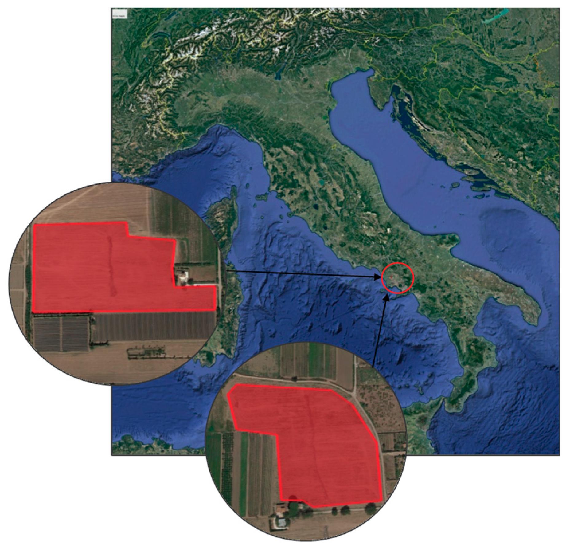
2.1. Test Site

The research was carried out in Frignano, located in Caserta province (Campania, Italy) (Figure 1). The area is characterized by a warm-temperate climate with an average annual temperature of 15.2 °C and 900 mm of annual cumulated precipitation, with the rainiest period occurring in winter and driest period in summer.

Processing tomato (Solanum lycopersicum L.) was cultivated in years 2017 (41°00′26.33″ N 14°10′13.93″ E) and 2018 (41°01′39.60″ N 14°10′32.87″ E) in two parcels of 4 ha each. Soil samples (three samples were averaged for analysis) were examined for assessing the main physical–chemical properties, including gravel (%), soil texture, bulk density (t/m³), pH and organic matter (%), at a depth of 15 cm. In 2018 soil characteristics were obtained by the soil map of Region Campania (pedological maps 1:50,000; http://agricoltura.regione.campania.it/pedologia/suoli.html). SPAW software (Soil–Plant–Air–Water; v6.02.75, United States Department of Agriculture-USDA, Washington, DC, USA) was used for assessing soil hydraulic properties, such as soil water retention, soil hydraulic conductivity, field capacity and plant available water.

Soil was ploughed at 40 cm depth, and tomato seedlings were transplanted on April 9 in continuous double rows with 33.5–40.0 cm space between plants, 50 cm between rows, 1.10–1.20 cm between double rows, with a final plant density of 32,000 and 33,500 plants/ha in year 2017 and 2018, respectively.

Fertilization was applied before transplanting (broadcast) with 120 kg/ha of diammonium phosphate (18-46-0) and 400 kg/ha of organic-mineral fertilizer (10-5-12); at transplanting (localized) with 160 kg/ha of diammonium phosphate and 20 kg/ha of seed sprint H5 (12-43-0).

Meteorological daily data of maximum and minimum temperature (°C), relative humidity (%), wind speed (m s⁻¹) and precipitation (mm) were collected at a complete weather station located in the study area for the two cropping seasons.

Plants were watered by light driplines, with 30 cm dripper spacing and 2 L/h flow rate at 1 bar.

Based on the farmer best knowledge, a total volume of 130 L/plant of water, corresponding to 4160 m³/ha, and 120 L/plant corresponding to 4020 m³/ha of irrigation was given throughout the growing period in 2017 and 2018, respectively. Such volumes were then considered as reference values against which the different estimation methods (AquaCrop, IRRISAT, integration of Sentinel 2A imagery into AquaCrop model) were tested.

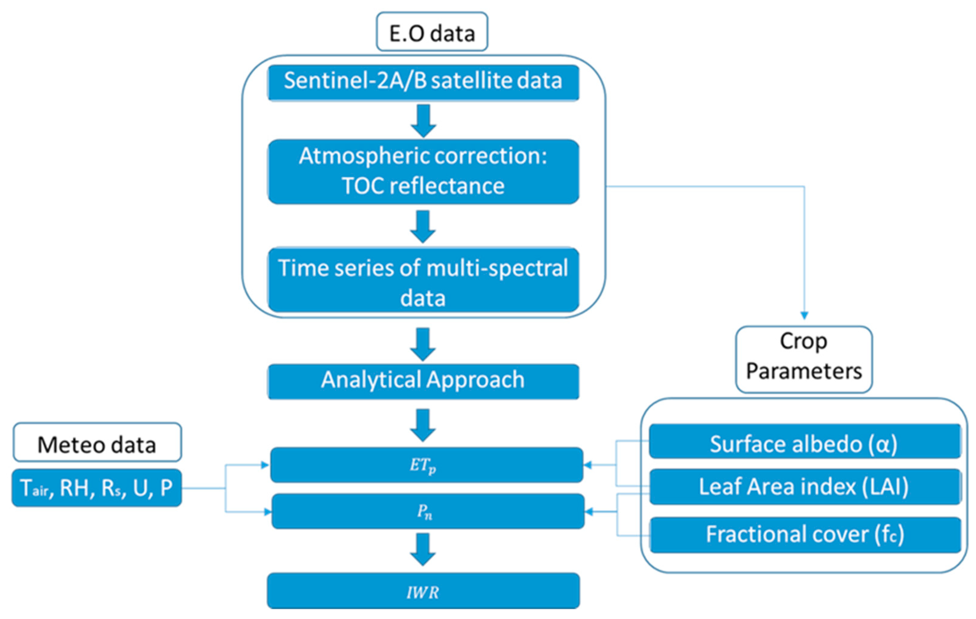
2.2. Satellite-Based Assessment of Crop Water Requirement: IRRISAT

The remote sensing technique employed is the one employed by IRRISAT, a satellite-based irrigation advisory service developed in Italy and operational since 2007 in Southern Italy [7]. The service aims at providing farmers and water managers with real time information on crop water needs, which are estimated by combining high resolution data from Earth Observation satellites with weather data for the calculation of crop water requirements. More recently, IRRISAT has been combined with numerical weather predictions for forecasting crop water needs up to five days in advance [19,20]. Information is delivered in near-real time (24 h) to users (farmers, Water User Association and water agencies) by means of a dedicated WebGIS accessible from PC, tablets and smartphones (https://www.irrisat.com/en/). In 2016, the operational irrigation advisory service of the Campania region has reached about 2000 farmers with a total irrigation area larger than 80,000 hectares: The achieved water saving has been estimated to be larger than 30% [7]. In 2016 the Italian Ministry of Agriculture has listed IRRISAT among the applicable methodologies for the estimation of the irrigation volume, complying with the EU Water Framework Directive.

The IRRISAT methodology is summarized in Figure 2. Crop potential evapotranspiration (ETp) is computed with the Penman–Monteith equation, with crop parameters albedo (α) and leaf area index (LAI) derived from processing Sentinel-2A/B images in the visible and infrared regions [7] while assuming fixed values for the stomatal resistance (sr ≈ 100 sm⁻¹) and crop height (hc = 0.4 m) for herbaceous crop [8]. Following this approach, the calculation of ETp requires standard meteorological data (daily air temperature, relative humidity, solar radiation, wind speed and precipitation), LAI and surface α.

The irrigation water requirement (IWR) is then calculated as the difference between ETp and the crop effective rainfall (Pn), according to the following equation:

IWR = ETp − Pn

(1)

It is assumed that capillary rise does not contribute to root zone soil moisture in the summer season, as usually occurs in the southern European regions. Runoff and deep drainage are assumed to be negligible considering the low amount of rainfall during the two growing seasons. Pn is obtained by reducing the precipitation above canopy (P) by a quantity that depends on canopy development, according to an empirical function of the LAI and the fractional vegetation cover fc, as reported in Vuolo et al. [7].

In this study, 10 and 21 multispectral high-resolution images from Sentinel-2A and 2B have been acquired during 2017 and 2018, respectively. The multi spectral instrument (MSI) on board of Sentinel-2A/2B captures data at 10, 20 and 60 m of spatial resolution over 13 spectral bands with a very high temporal resolution of five days at the equator. Individual Sentinel-2 granules Level-1C (processed at the top-of-atmosphere reflectance) were acquired from Copernicus Open Access Hub (https://scihub.copernicus.eu/), already ortho-rectified in UTM/WGS84 (image tiles of 100 × 100 km²). The information gathered by Sentinel-2 system (orbit, attitude, date accuracy and viewing directions of all detectors) are exploited for geolocating all Sentinel-2 pixels with an accuracy of about 11 m for about 97% of the cases, which is about the size of one Sentinel-2 pixel. The standard need for multi-temporal registration errors is 0.3 pixels, and the current performances show that for more than 50% of the cases, the performance does not meet that requirement. The resolution is estimated to be three times the registration error, thus the resolution Sentinel-2 time series is around 30 m.

Level-1C products were processed into Level-2A-Bottom-of-Atmosphere (BoA) reflectance-data using the ESA’s Sen2Cor v2.5.5 tool (http://step.esa.int/main/third-party-plugins-2/sen2cor/sen2cor_v2-5-5/). Sen2Cor tool performs the atmospheric, terrain and cirrus correction of Top-Of-Atmosphere Level 1C input data, and creates Bottom-Of-Atmosphere, optionally terrain and cirrus corrected reflectance images; additional, aerosol optical thickness, water vapor, scene classification maps and quality indicators for cloud and snow probabilities.

In order to obtain homogeneous and comparable products as time series, all value-added products (LAI, α and fc) are calculated based on atmospherically corrected Level-2A data. LAI and fc are calculated by S2ToolBox [21], an artificial neural network (ANN) algorithm, trained by using radiative transfer simulations from PROSPECT [22] and SAIL [23] models, and tailored for Sentinel-2 data. The algorithm requires eight Sentinel-2 spectral bands (B3–B7, B8a, B11 and B12) at 10 and 20 m (pixel size), which are all resampled to 10 m to derive LAI and fc. Experimental studies have shown the accuracy of this approach for LAI estimation in different environments and crops [24,25]. In this study, average and variance of LAI and fc at parcel scale were assessed by taking a minimum of 50 pixels falling within each parcel, after excluding pixels affected by boundary effects or cloudiness, according to the quality indicator provided by S2ToolBox.

The broadband surface albedo has been calculated, when the observed surface is considered as Lambertian, as the integration of at-surface reflectance across the shortwave spectrum [26], as shown in equation:

$$\alpha ={\sum }_{bi}\left|{\rho }_{bi}·{\omega }_{bi}\right|$$

(2)

where α is albedo, ρ_bi is surface reflectance for a given band bi at Level-2A Sentinel-2 surface reflectance, ω_bi is the weighting coefficient representing the solar radiation fraction derived from the solar irradiance spectrum [26] within the spectral range (spectral response curves) for bands bi and is calculated as equation:

$${\omega }_{bi}=\frac{{{\displaystyle \int }}_{L{O}_{bi}}^{U{P}_{bi}}{R}_{s\lambda }·d\lambda }{{{\displaystyle \int }}_{0.4}^{2.4}{R}_{s\lambda }·d\lambda }$$

(3)

where R_sλ is extra-terrestrial irradiance for wavelength λ (μm); and UP_bi and LO_bi are upper and lower wavelength bounds for Sentinel-2A/B band bi, respectively.

2.3. Model-Based Assessment of Crop Water Requirement: AquaCrop

AquaCrop simulates crop yield in four steps: Crop development, crop transpiration, biomass production and yield formation. It calculates the daily soil water balance and divides evapotranspiration into soil evaporation and crop transpiration. AquaCrop describes the foliage development of the crop by the canopy cover (CC), that is formally equivalent to the fractional cover (fc) estimated by Sentinel-2 imagery, i.e., it is the fraction of soil surface covered by the green canopy. Hereinafter, we use the two terms canopy cover (CC) and fractional cover (fc) just to distinguish the two variables, respectively derived with AquaCrop and Sentinel-2 imagery.

Transpiration is a function of CC, while evaporation is proportional to the area of soil not covered by vegetation. The CC is multiplied by reference evapotranspiration (ETo), determined by the FAO Penman–Monteith equation, and the crop coefficient (Kc) to calculate potential crop transpiration. Actual transpiration (Ta) is calculated starting from potential one by accounting for water stress. Then, Ta is used for the calculation of crop biomass though its multiplication with water productivity normalized for climate. By using a harvest index (HI), crop yield is obtained by the biomass. To describe the effect of water stress, the model considers different thresholds of water available to the root zone. The first affects leaf canopy expansion (slowing down); the second threshold affects canopy senescence (quickening); the third is referred to as stomata closure (increase) and so to transpiration. Stress coefficients (Ks) range between 1 (no stress) and 0 (complete stress) and are multiplicative factors of the target process.

Model parameters are grouped into two classes: Conservative and non-conservative. Conservative parameters are not dependent on local and management conditions: Canopy growth (CGC) and canopy decline (CDC) coefficients; full canopy crop transpiration coefficient (Kc); biomass WP and soil water depletion thresholds. Non-conservative parameters vary depending on crop and field management, soil type, and climate (sowing date and density, length of crop cycle and phenological stages, maximum canopy cover, etc.). Such parameters can be either retrieved from AquaCrop literature or calibrated by the user (e.g., by means of field experiments). Main AquaCrop outputs are crop production (biomass and yield) and crop water use.

AquaCrop Implementation

In this study, a limited number of AquaCrop parameters were partly calibrated with field observations, including management information: Transplant dates and densities, flowering date and duration, starting of senescence, maturity, and final yield were used for local calibration of the model. For simulating irrigation, the model was set in net irrigation requirement mode, which estimates the crop water requirement based on a selected threshold of allowed root zone (water) depletion (RZD). In order to reproduce the irrigation method adopted by the farmer, drip irrigation was simulated to ensure that RZD was always above 50% of the readily available water (RAW).

2.4. Assimilation-Based Assessment of Crop Water Requirement

The third method for assessing crop water requirements was based on the integration of Sentinel-2 crop derived data with AquaCrop. The fractional cover (fc) estimated by Sentinel-2 has been sequentially assimilated into AquaCrop, by direct insertion, in place of the canopy cover (CC) simulated by the model. The sequential direct insertion is applied under the assumption that a continuous update of one crop model state based on remote observations can reduce the biases induced by the model simplifications of the processes and environmental conditions influencing the crop growth dynamics.

Crop CC simulated by AquaCrop along the growing season and the fc values measured by satellite were compared and the differences were statistically analyzed by means of the Pearson correlation coefficient (r), root mean square error (RMSE%), Nash–Sutcliffe model efficiency coefficient (EF) and Willmott index of agreement (d).

3. Results and Discussion

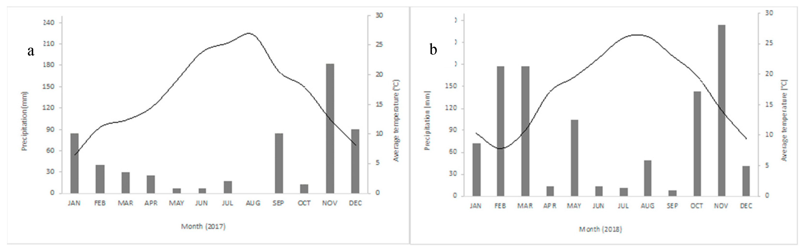
3.1. Test Site Characteristics

The parcel cultivated in 2017 had a Vitric Phaeozems (Eutric) soil (WRB classification), with a loamy texture (USDA classification), while soil was Vitric Cambisols with a loamy-sand texture in 2018. Soils were both deep, well drained and with no fertility constraints (

Table 1. Main soil characteristics of the two soils.

Parameter	Unit	2017	2018
Texture		Loam	Silty loam
Gravel	(vol%)	<5	<5
Saturation	(vol%)	52	46
Field Capacity	(vol%)	29	33
Wilting Point	(vol%)	10	13
Cation Exchange Capacity	(meq/100g)	32	24
Bulk Density	(t/m3)	1.1	1.3
pH in H2O	U.pH	6.9	7.1
Organic Matter	(%)	2.6	2.7

).

Considering the climatology of the study area, average temperature of 15.2 °C and precipitation of 900 mm (period 1982–2012), year 2017 was relatively dry, with a cumulated rainfall of 579 mm and 16.6 °C of average temperature, whereas 2018 was relatively wet and warm, with 1047 mm of rainfall and an average temperature of 17.25 °C (Figure 3). Observed processing tomato yield (expressed in dry matter) was 7.20 t/ha in 2017 and 7.35 t/ha in 2018.

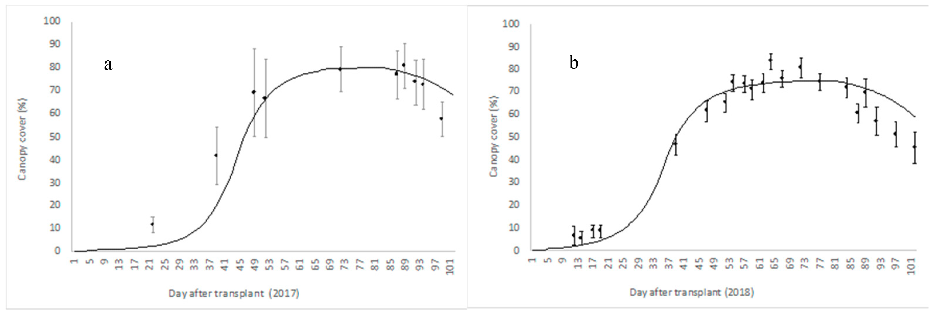
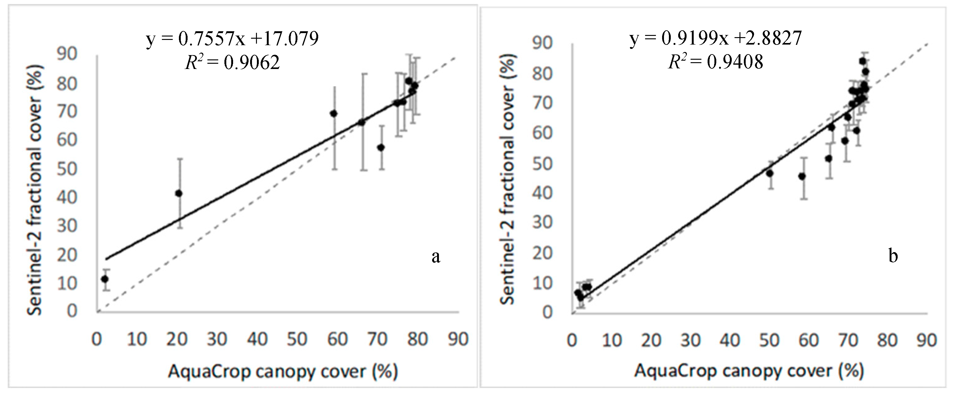
3.2. AquaCrop Calibration and Implementation

AquaCrop parameters were calibrated to obtain the best fit between field observations and simulations, both in 2017 and 2018 (

Table 2. Input crop file used for AquaCrop simulations (HI: Harvest index, GDD: Growing degree days).

Crop Parameter	Unit	Value
Max canopy cover	GDD	686
Flowering	GDD	612
Flowering duration	GDD	531
Length building up HI	GDD	448
Senescence	GDD	1013
Maturity	GDD	1358
Max rooting depth	GDD	612
Initial canopy cover	%	0.64
Maxi canopy cover	%	75
Reference HI	%	63
Base temperature	°C	5
Upper temperature	°C	30
Canopy expansion Upper		0.15
Canopy expansion Lower		0.55
Stomatal closure		0.5
Early canopy senescence		0.7

). AquaCrop simulated yields were 7.23 and 7.60 t/ha (dry weight) in 2017 and 2018, with an error of 0.42% and 3.40%, respectively (

Table 3. Crop and water balance variables (Tr: Crop transpiration, E: Soil evaporation, ETp: Potential evapotranspiration, IWR: Irrigation water requirement, WP_ET: Evapotranspiration water productivity, WP_IWR: Irrigation water requirement water productivity).

		Yield (t/ha)	Tr (mm)	E (mm)	ETp (mm)	IWR (mm)	WPET (kg/m3)	WPIWR (kg/m3)
2017	Observed	7.20				416		1.73
	IRRISAT				450	450
	AquaCrop	7.23	345	192	537	461	1.35	1.57
	Assimilation	8.23	372	165	537	461	1.52	1.79
2018	Observed	7.35				402		1.82
	IRRISAT				349	298
	AquaCrop	7.60	291	137	428	332	1.78	2.29
	Assimilation	7.34	273	139	412	317	1.78	2.31

). The growth of the green canopy simulated by the model was compared with the fc values observed by IRRISAT. In both seasons the simulated growing curve fitted well with the satellite observations, although an underestimation for the initial canopy cover (late April–early May) and an overestimation during the last part of the growing season (July) was observed (Figure 4). Nevertheless, the statistical analysis (RMSE, EF, d) showed a very good agreement between simulated CC and fc, which correlation was highly significant in both years (α = 0.001;

Table 4. Evaluation of canopy cover simulation results: Number of observations/simulations (n), Pearson correlation coefficient (r), root mean square error (RMSE%), Nash–Sutcliffe model efficiency coefficient (EF) and Willmott index of agreement (d).

	n	r	RMSE	EF	d
2017	10	0.95	9.10	0.8	0.96
2018	22	0.97	8.10	0.91	0.98

; Figure 5). In 2017 the spatial variability of the crop canopy within the study parcel was larger than in 2018, as testified by the larger variance of the fc values retrieved in 2017.

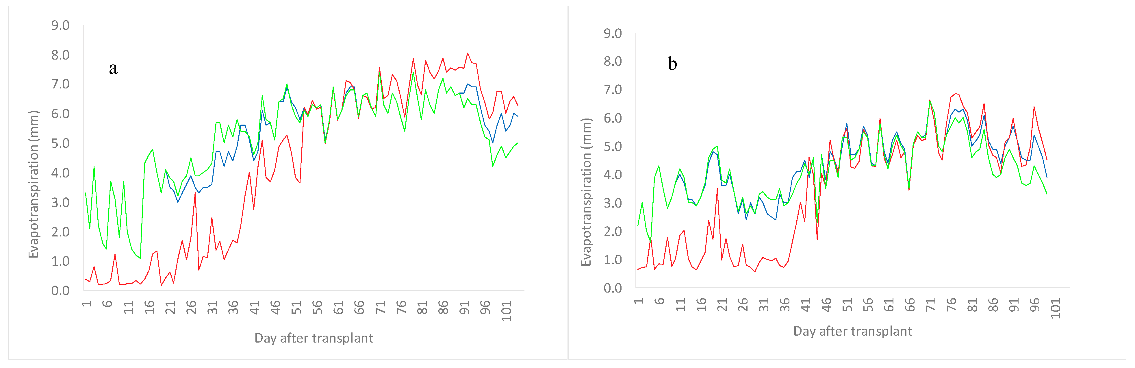
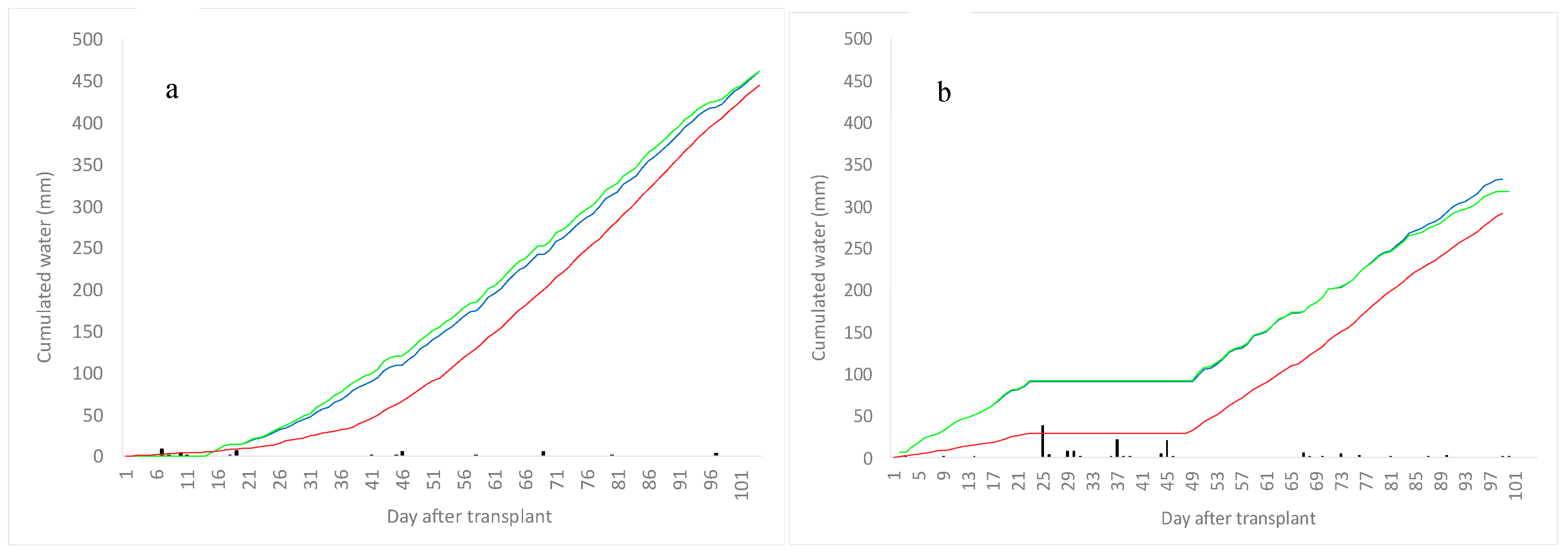
3.3. Estimation of Crop Water Irrigation Requirements

During the 2017 crop growing season, spanning from June 9th to July 20th, the accumulated rainfall was 40.4 mm, the estimated reference evapotranspiration (ETo) was 553 mm, while crop transpiration (Tr) and soil evaporation (E) estimated by AquaCrop were 345 and 192 mm, respectively. In such conditions, AquaCrop modeled an irrigation water requirement (IWR) of 461 mm corresponding to 144 L/plants.

In year 2018, wetter conditions occurred, with an accumulated rainfall of 125 mm and an estimated ETo of 439 mm. Under such conditions, both crop Tr (291 mm) and E (137 mm) were lower. Accordingly, a lower IWR, 332 mm, was estimated by the model. Being the final yields very similar, the consequent evapotranspiration (WP_ET) was higher in 2018 than 2017 (Tab 3).

In Figure 6, three different daily ETp series were compared, respectively produced by calibrated AquaCrop, IRRISAT and AquaCrop after replacing CC with fc estimated by IRRISAT.

The agreement between AquaCrop and IRRISAT ETp estimates is excellent in the mid-season stage, between about the 50th and 85th day after transplant, when the crop canopy is fully developed. This result is remarkable considering that IRRISAT is fully based on remote observations weather data, and not relying on field or crop data. Moreover, IRRISAT predictions are not based on a continuous assessment of the crop dynamics, rather it provides ETp estimates based on crop parameters retrieved from the last available image, thus with a delay of five or more days, depending on the sky conditions (i.e., cloudiness).

In the initial stage and in the crop development stage (first 50 days after transplant), before canopy is fully developed, the estimation of ETp in AquaCrop is higher than the one determined by IRRISAT. This is due to the conceptually different calculation schemes: Whilst IRRISAT has a resistance-based approach in the Penman–Monteith linked to the LAI at the pixel scale (according to the “big leaf” schematization), AquaCrop has a crop coefficient approach for soil evaporation depending on soil properties. Diversely, with growing LAI and soil cover, the two estimates converge toward very similar values of ETp, hence irrigation requirements.

In the senescence stage, after about the 85th day from transplant, the values of ETp derived by means of the two methods slightly diverge again, with higher ETp for IRRISAT respect to AquaCrop, again due to the difference between the LAI-based approach of the first one and the crop coefficient of the second one. Furthermore, AquaCrop explicitly consider the transpiration reduction associated with the senescence, which cannot be fully predicted by the reduction of the observed LAI applied into the Penman–Monteith equation.

The canopy cover fc maps retrieved from Sentinel-2 imagery can be more effectively employed for constraining AquaCrop predictions to the actual observed crop growth and for assessing its spatial variability. In this study we applied a simple assimilation technique, known in the literature as “direct” insertion [27], consisting in replacing the model state variable CC with the remotely retrieved variable fc. As displayed in Figure 6, AquaCrop ETp estimates after direct insertion are essentially equal to the calibrated AquaCrop, except for the development and senescence stages, when the average fc sensibly deviates from the model calibrated growth curve. As illustrated in Table 3, fc direct insertion does not affect the cumulative ETp, rather it affects its partitioning in transpiration (Tr) an evaporation (E), with a slight increase in Tr and a decrease in E. In 2018, instead, fc direct insertion implies a slight reduction of ETp, mainly associated with a reduction of Tr. Correspondingly, tomato yield was overestimated compared with the observed and the calibrated values in 2017 (+14.3%), while slightly underestimated in 2018 (−1.03%). This result confirmed that sequential assimilation of one state variable does not necessarily improve the prediction performance of all model state variables. In this sense, more complex sequential assimilation techniques are needed, in order to account for the structure of the observation and prediction errors [28], as well of the atmospheric forcing [29].

The impact of the direct insertion in terms of irrigation water requirement (IWR) is null in 2017, while it determines a 5% decrease in 2018. As illustrated in Figure 7, also the temporal pattern of IWR is almost unchanged in the two simulated seasons. A potential water saving of 70 mm could be achieved in 2018 according to AquaCrop, by accounting for the effective contribution of the summer rainfall (125 mm) to the soil water deficit.

Looking again at Table 3, it is interesting to note that IRRISAT, despite the significant reduction of the cumulative ETp both in 2017 (16%) and 2018 (19%) compared with the calibrated AquaCrop, predicts cumulative IWR just 3% smaller in 2017 and 11% smaller in 2018 than the calibrated AquaCrop. As illustrated in Figure 7, this reduction is essentially due to the initial and development stage, when AquaCrop, differently form IRRISAT, accounts for the soil evaporation in the IWR assessment. After the crop is fully developed, the cumulative IWR curves are almost parallel, testifying the good agreement of the remotely assessed daily IWR with AquaCrop.

4. Conclusions

Sentinel-2 imagery can be effectively exploited for monitory canopy growth of tomato crops in open field. Irrigation advisory services, such as IRRISAT, which are only based on crop data retrieved by Sentinel-2 and weather data, can provide a reliable assessment of crop water requirements of tomato field crops especially when crop canopy is fully developed. It should be considered that IRRISAT does not require input data concerning the soil or crop phenology, since it is entirely based on crop growth monitoring from space. Hence, integrating Sentinel-2 imagery with a crop growth model such as AquaCrop can be an effective strategy for assessing crop water requirement in the initial and development stage of the crop, as well as for identifying the senescence stage. Further, being the satellite imagery a spatial information, the integration into a crop model can help in assessing crop water requirement at field or higher scales, i.e., at territorial level. Thus, a sequential assimilation can be used to support irrigation planning by Irrigation and Land Reclamation consortia. In this study a simple direct insertion method has been applied for assimilating canopy cover retrieved by Sentinel-2 imagery into AquaCrop, which does not guarantee an optimal model-data integration. Additional studies are required for testing more advanced data assimilation techniques, accounting for the structure of the model state and observation errors.

References

1. Altobelli, F.; Cimino, O.; Natali, F.; Orlandini, S.; Gitz, V.; Meybeck, A.; Marta, A.D. Irrigated farming systems: Using the water footprint as an indicator of environmental, social and economic sustainability. J. Agric. Sci. 2018, 156, 711–722. [Google Scholar] [CrossRef]
2. Tsakmakis, I.D.; Zoidou, M.; Gikas, G.D.; Sylaios, G.K. Impact of Irrigation Technologies and Strategies on Cotton Water Footprint Using AquaCrop and CROPWAT Models. Environ. Process. 2018, 5, 181–199. [Google Scholar] [CrossRef]
3. Kustas, W.; Anderson, M. Advances in thermal infrared remote sensing for land surface modeling. Agric. For. Meteorol. 2009, 149, 2071–2081. [Google Scholar] [CrossRef]
4. Anderson, M.C.; Norman, J.M.; Mecikalski, J.R.; Otkin, J.A.; Kustas, W.P. A climatological study of evapotranspiration and moisture stress across the continental United States based on thermal remote sensing: 2. Surface moisture climatology. J. Geophys. Res. 2007, 112, D11112. [Google Scholar] [CrossRef]
5. Karimi, P.; Bastiaanssen, W.G.M.; Molden, D. Water Accounting Plus (WA+)—A water accounting procedure for complex river basins based on satellite measurements. Hydrol. Earth Syst. Sci. 2013, 17, 2459–2472. [Google Scholar] [CrossRef]
6. Drusch, M.; Del Bello, U.; Carlier, S.; Colin, O.; Fernandez, V.; Gascon, F.; Hoersch, B.; Isola, C.; Laberinti, P.; Martimort, P. Sentinel-2: ESA’s optical high-resolution mission for GMES operational services. Remote Sens. Environ. 2012, 120, 25–36. [Google Scholar] [CrossRef]
7. Vuolo, F.; D’Urso, G.; De Michele, C.; Bianchi, B.; Cutting, M. Satellite-based irrigation advisory services: A common tool for different experiences from Europe to Australia. Agric. Water Manag. 2015, 147, 82–95. [Google Scholar] [CrossRef]
8. D’Urso, G. Current Status and Perspectives for the Estimation of Crop Water Requirements from Earth Observation. Ital. J. Agron. 2010, 5, 107–120. [Google Scholar]
9. Casa, R.; Varella, H.; Buis, S.; Guerif, M.; de Solan, B.; Frederic, B. Forcing a wheat crop model with LAI data to access agronomic variables: Evaluation of the impact of model and LAI uncertainties and comparison with an empirical approach. Eur. J. Agron. 2012, 37, 1–10. [Google Scholar] [CrossRef]
10. Steduto, P.; Hsiao, T.C.; Raes, D.; Fereres, E. Aquacrop-the FAO crop model to simulate yield response to water: I. concepts and underlying principles. Agron. J. 2009, 101, 426–437. [Google Scholar] [CrossRef]
11. Raes, D.; Steduto, P.; Hsiao, T.C.; Fereres, E. AquaCropThe FAO Crop Model to Simulate Yield Response to Water: II. Main Algorithms and Software Description. Agron. J. 2009, 101, 438–447. [Google Scholar] [CrossRef]
12. Linker, R.; Ioslovich, I. Assimilation of canopy cover and biomass measurements in the crop model AquaCrop. Biosyst. Eng. 2017, 162, 57–66. [Google Scholar] [CrossRef]
13. Jin, X.; Kumar, L.; Li, Z.; Xu, X.; Guijun, Y.; Wang, J. Estimation of Winter Wheat Biomass and Yield by Combining the AquaCrop Model and Field Hyperspectral Data. Remote Sens. 2016, 8, 972. [Google Scholar] [CrossRef]
14. Silvestro, P.C.; Pignatti, S.; Pascucci, S.; Yang, H.; Li, Z.; Guijun, Y.; Huang, W.; Casa, R. Estimating Wheat Yield in China at the Field and District Scale from the Assimilation of Satellite Data into the Aquacrop and Simple Algorithm for Yield (SAFY) Models. Remote Sens. 2017, 9, 509. [Google Scholar] [CrossRef]
15. Jin, X.; Liu, S.; Baret, F.; Hemerlé, M.; Comar, A. Estimates of plant density of wheat crops at emergence from very low altitude UAV imagery. Remote Sens. Environ. 2017, 198, 105–114. [Google Scholar] [CrossRef] [Green Version]
16. Jin, X.; Kumar, L.; Li, Z.; Feng, H.; Xu, X.; Guijun, Y.; Wang, J. A review of data assimilation of remote sensing and crop models. Eur. J. Agron. 2018, 92, 141–152. [Google Scholar] [CrossRef]
17. Zhao, Y.; Chen, S.; Shen, S. Assimilating remote sensing information with crop model using Ensemble Kalman Filter for improving LAI monitoring and yield estimation. Ecol. Model. 2013, 270, 30–42. [Google Scholar] [CrossRef]
18. Trombetta, A.; Iacobellis, V.; Tarantino, E.; Gentile, F. Calibration of the AquaCrop model for winter wheat using MODIS LAI images. Agric. Water Manag. 2016, 164, 304–316. [Google Scholar] [CrossRef]
19. Pelosi, A.; Medina, H.; Villani, P.; D’Urso, G.; Chirico, G.B. Probabilistic forecasting of reference evapotranspiration with a limited area ensemble prediction system. Agric. Water Manag. 2016, 178, 106–118. [Google Scholar] [CrossRef]
20. Chirico, G.B.; Pelosi, A.; De Michele, C.; Bolognesi, S.F.; D’Urso, G. Forecasting potential evapotranspiration by combining numerical weather predictions and visible and near-infrared satellite images: An application in southern Italy. J. Agric. Sci. 2018, 19, 702–710. [Google Scholar] [CrossRef]
21. Garrigues, S.; Lacaze, R.; Baret, F.J.; Morisette, J.T.; Weiss, M.; Nickeson, J.E.; Fernandes, R.; Plummer, S.; Shabanov, N.V.; Myneni, R.B.; et al. Validation and intercomparison of global Leaf Area Index products derived from remotesensing data. Geophys. Res. 2008, 113. [Google Scholar] [CrossRef]
22. Jacquemoud, S.; Baret, F. PROSPECT: A model of leaf optical properties spectra. Remote Sens. Environ. 1990, 34, 75–91. [Google Scholar] [CrossRef]
23. Verhoef, W. Light scattering by leaf layers with application to canopy reflectance modeling: The SAIL model. Remote Sens. Environ. 1984, 16, 125–141. [Google Scholar] [CrossRef] [Green Version]
24. Atzberger, C.; Berger, K. Spatially constrained inversion of radiative transfer models for improved LAI mapping from future Sentinel-2 imagery. Remote Sens. Environ. 2012, 120, 208–218. [Google Scholar] [CrossRef]
25. D’Urso, G.; Calera Belmonte, A. Operative approaches to determine crop water requirements from earth observation data: Methodologies and applications. AIP Conf. Proc. 2006, 852, 14–25. [Google Scholar]
26. Thuillier, G.; Hersé, M.; Labs, D.; Foujols, T.; Peetermans, W.; Gillotay, D.; Simon, P.C.; Mandel, H. The solar spectral irradiance from 200 to 2400 nm as measured by the solspec spectrometer from the atlas and Eureca missions. Sol. Phys. 2003, 214, 1–22. [Google Scholar] [CrossRef]
27. Chirico, G.B.; Medina, H.; Romano, N. Kalman filters for assimilating near-surface observations in the Richards equation. I: Retrieving state profiles with linear and nonlinear numerical schemes. Hydrol. Earth Syst. Sci. 2014, 18, 2503–2520. [Google Scholar] [CrossRef]
28. Medina, H.; Romano, N.; Chirico, G.B. Kalman filters for assimilating near-surface observations into the Richards equation—Part 2: A dual filter approach for simultaneous retrieval of states and parameters. Hydrol. Earth Syst. Sci. 2014, 18, 2521–2541. [Google Scholar] [CrossRef]
29. Pelosi, A.; Medina, H.; Van den Bergh, J.; Vannitsem, S.; Chirico, G.B. Adaptive Kalman filtering for postprocessing ensemble numerical weather predictions. Mon. Weather Rev. 2017, 145, 4837–4854. [Google Scholar] [CrossRef]
Figure 1. Localization of the pilot area and the two experimental fields.
Agronomy 09 00404 g001
Figure 2. Flowchart shows dataset and processing procedure required to estimate crop potential evapotranspiration (ETp), and irrigation water requirements (IWR), Earth Observation-based direct FAO-56 Penman-Monteith equation method. Legend: Ta = air temperature, RH = relative humidity; Rs = solar radiation; U = wind speed; P = precipitation.
Agronomy 09 00404 g002
Figure 3. Temperature (line) and precipitation (bars) in the experimental area in year 2017 (a) and 2018 (b).
Agronomy 09 00404 g003
Figure 4. Canopy cover of tomato simulated by AquaCrop, after calibration with field data (line) and corresponding fractional cover values (dots) retrieved by Sentinel-2 imagery during 2017 (a) and 2018 (b) growing seasons, with corresponding standard deviations.
Agronomy 09 00404 g004
Figure 5. Linear correlation between tomato canopy cover simulated by AquaCrop and fractional cover retrieved by Sentinel-2 imagery in 2017 (a) and 2018 (b). Standard deviation (bars) and 1:1 line (dashed line) are reported.
Agronomy 09 00404 g005
Figure 6. Crop evapotranspiration estimated by AquaCrop (blue), IRRISAT (red) and direct insertion (green) of fc retrieved by Sentinel-2 imagery into AquaCrop, in 2017 (a) and 2018 (b).
Agronomy 09 00404 g006
Figure 7. Cumulated irrigation water requirement (mm) estimated by the three methods: AquaCrop (blue), IRRISAT (red) and direct insertion (green) of fractional cover retrieved by Sentinel-2 imagery into AquaCrop, in 2017 (a) and 2018 (b). Rainfall is also plotted (histograms).
Agronomy 09 00404 g007