A Novel Approach for Cloud Detection in Scenes with Snow/Ice Using High Resolution Sentinel-2 Images

1
School of Geology Engineering and Geomatics, Chang’an University, Xi’an 710064, China
2
Shaanxi Key Laboratory of Land Consolidation and Rehabilitation, Chang’an University, Xi’an 710064, China
3
Track and Tunnel Branch Institute, Anhui Transport Consulting & Design Institute Co.,Ltd., Anhui 233088, China
*
Author to whom correspondence should be addressed.
†
The two authors contributed equally to this paper.
Atmosphere 2019, 10(2), 44; https://0-doi-org.brum.beds.ac.uk/10.3390/atmos10020044
Submission received: 14 December 2018
/
Revised: 19 January 2019
/
Accepted: 19 January 2019
/
Published: 23 January 2019
(This article belongs to the Special Issue Remote Sensing of Clouds)
Abstract
:The recognition of snow versus clouds causes difficulties in cloud detection because of the similarity between cloud and snow spectral characteristics in the visible wavelength range. This paper presents a novel approach to distinguish clouds from snow to improve the accuracy of cloud detection and allow an efficient use of satellite images. Firstly, we selected thick and thin clouds from high resolution Sentinel-2 images and applied a matched filter. Secondly, the fractal digital number-frequency (DN-N) algorithm was applied to detect clouds associated with anomalies. Thirdly, spatial analyses, particularly spatial overlaying and hotspot analyses, were conducted to eliminate false anomalies. The results indicate that the method is effective for detecting clouds with various cloud covers over different areas. The resulting cloud detection effect possesses specific advantages compared to classic methods, especially for satellite images of snow and brightly colored ground objects with spectral characteristics similar to those of clouds.
1. Introduction
Clouds and snow cover are spectrally distinguishable despite having similar reflectance spectra in the visible-light range. The existence of clouds in remotely sensed images obscures surface features. Therefore, accurate cloud cover detection is vital for earth observation using remote sensing data processing systems.
Bunting et al. discussed the reflectance properties of snow and clouds in the visible and near-infrared wavelength regions [1]. They analyzed imagery in pairs, with one set in the visible spectrum and the other in the near-infrared spectrum, and presented a method that utilized data from the near-infrared spectrum to analyze clouds over snow- or ice-covered regions. At these wavelengths, snow appears relatively dark while clouds are highly reflective. However, in rugged terrain, snow in the shadows can be darker than soil or vegetation in the sunlight, so that snow mapping in the mountains is not so easily accomplished [2]. Salomonson et al. [3] and Homan et al. [4] detected snow cover by normalized difference snow index (NDSI). This method reduced misjudgments considerably, but cloud shadows and liquid water can produce high values of NDSI and thus be misidentified as snow or ice [5]. Furthermore, cloud cover in some Antarctic images, especially on the Antarctic Peninsula, leads to the classification of clouds as rock exposure by the NDSI technique, as the two are indiscernible using this methodology [6]. Beaudoin [7] and Wang et al. [8] detected clouds through k-means algorithm. It was found that the algorithm gives better results but does not take into account the spatial information. Hégarat–Mascle et al. detected clouds through Markov random fields using physical properties such as cloud shadow shapes and location correlation [9]. Although the technique provides good cloud detection results for high-resolution images, the results are affected by the solar zenith angle of shadows. The Fmask algorithm was originally developed to mask clouds, cloud shadows, and snow for Landsat 4 to Landsat 7. Using an object-based cloud and cloud shadow matching algorithm, it can provide masks for clouds, cloud shadows, and snow for each individual image [10,11]; however, Fmask may fail to detect clouds in images showing heterogeneous surface reflectance, because the algorithm uses a scene-based threshold and applies the same threshold to all pixels in the image [12].
In addition, texture is an important feature, as it reflects not only the gray statistical information from the image but also the structures of the ground features and relationships among the spatial arrangement of the objects. Thus, it can be used to distinguish different objects [13]. The edges of cloud areas are usually blurred and rounded, with slow gradient changes. Meanwhile, snow-covered land is affected by topography (man-made terrain, mountains, and vegetation), the edges are usually sharp, and the gray gradient changes dramatically [14]. Many scientists have done considerable works to improve the accuracy of cloud or snow detection [15,16,17,18]. However, most of the present texture-based algorithms assume that there is no snow in the cloudy images or no clouds in the snow covered images [18]. Besides, there are many types of texture features, and using more features does not naturally result in higher accuracy because of the Hughes effect [19]. Moreover, using more features also results in a high computational cost [17]. Therefore, this method still has many uncertainties and poor adaptability [20]. Using textures to distinguish between snow and cloud remains challenging.
Sen2Cor is a Level-2A processor whose main purpose is to correct single-date Sentinel-2 Level-1C Top-Of-Atmosphere (TOA) products from the effects of the atmosphere in order to deliver a Level-2A Bottom-Of-Atmosphere (BOA) reflectance product. Additional outputs are an Aerosol Optical Thickness (AOT) map, a Water Vapour (WV) map and a Scene Classification (SCL) map with Quality Indicators for cloud probabilities (QI) [21,22]. However, there are still some challenges to be solved. Kukawska E. et al. revealed a problem with the resulting cloud cover mask [23]. It was found that three classes from the mask representing clouds recognized with low, medium, and high probability present an incorrect classification of surfaces (e.g., buildings, asphalt, and snow) which tend to have a higher reflectance than surrounding objects. This results in masking out a considerable part of a high reflectance area when combining multitemporal observations. Additionally, the Sentinel-2 Level 1C cloud mask product exhibits the worst performance in the following cases: In the correspondence of snowy surfaces (wrongly identified as cirrus/opaque clouds); in the correspondence of bright surfaces, such as sand and white buildings (sometimes identified as opaque clouds); over high elevation surfaces with particular dry atmospheric conditions (sometimes confused as cirrus clouds) [24]. Furthermore, the Sen2cor scene classification cloud masking method has the same issues as the threshold method, it could be improved by better and more carefully selecting the thresholds. Unfortunately, since the clouds are masked by the Sen2cor plugin, you cannot change or improve the detection and masking in contrast to the threshold method [25].
This study proposes a matched filtering (MF) method that uses the DN-frequency (DN-N) fractal model and spatial analysis of the point pattern method to separate clouds from snow and ice in brightly colored areas. The aim of this method is to extend the techniques described previously, thereby enhancing the visual comprehension and enabling a quantitative and accurate interpretation. This approach has potential advantages for the extraction of anomaly information relative to classic cloud detection approaches.
2. Materials and Methods
2.1. Proposed Method Framework
The flowchart of the proposed algorithm is illustrated in Figure 1. The algorithm consists of three main steps: Data preparation, cloud detection based on pixel values, and clustering levels. The nearest neighbor method was used to resample the images at 10 m resolution in data preparation section [26]. In addition, the method proposed in this study uses matched filtering and DN-N fractal characteristics to detect clouds. This method can be used to solve the problem of snow being misclassified as clouds, as frequently occurred using traditional detection methods. Finally, clustering levels eliminate salt-and-pepper noise generated by the brightly surface, greatly improving the accuracy of cloud detection. The algorithm is introduced below in detail.
2.2. Study Area and Data Source
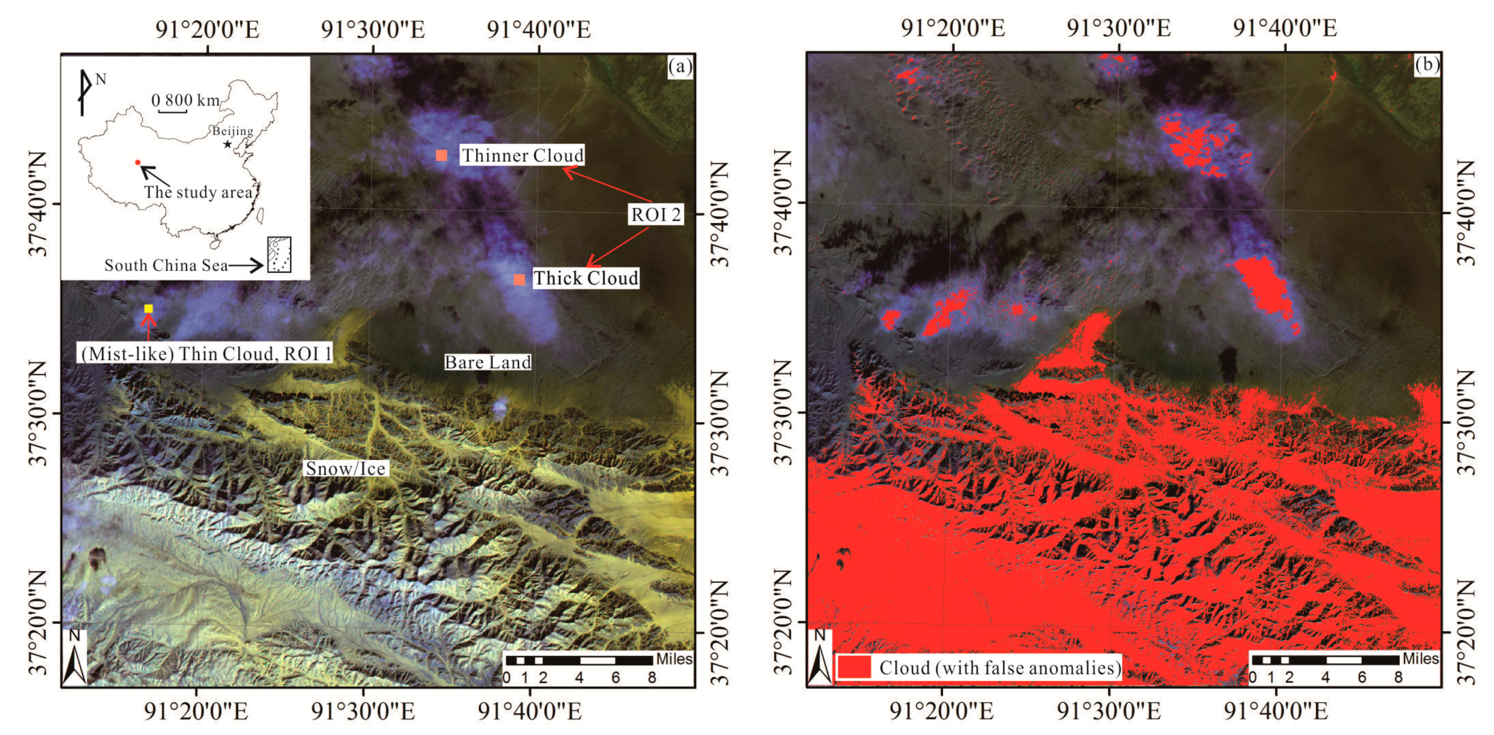
In this study, Sentinel-2 data were acquired from the European Space Agency (ESA) Copernicus Open Access Hub (https://scihub.copernicus.eu/). The data were sourced from high resolution Sentinel-2 Level-1C images. The Level-1C product results from using a Digital Elevation Model (DEM) to project the image in cartographic geometry. Per-pixel radiometric measurements are provided in Top Of Atmosphere (TOA) reflectances along with the parameters to transform them into radiances [11,24,26,27]. We selected all bands in Sentinel-2 images (including visible and near-IR wavelengths), in order to maximize band characteristics and avoid band information loss. Although clouds and snow cover show similar reflectance in the satellite imagery, the real reflectance of clouds and snow are still different in each band [28], which contains some important diagnostic absorption and reflection features of clouds and snow, therefore, all bands were selected for the proposed method. Sentinel-2 images are multiresolution data having bands at 10 m, 20 m, and 60 m spatial resolution, and we resample all the 20 m and 60 m bands to 10 m resolution [29]. We applied the algorithm to a dataset acquired in different periods or times with snow and brightly colored ground objects on the underlying surface. In the method section we show the results obtained for a typical image (only one case study, the typical image shows thick and thin clouds as well as snow cover); results obtained on the remaining case studies are presented and discussed in the results and discussion sections. The typical image cloud coverage in Figure 2a is 5.7% (ingestion data: 19 February 2018, relative orbit number: 33), although this image had a relatively low cloud coverage level, the scene image was typical. In remote sensing interpretations, the desert, snow, glaciers, other ground objects, and clouds, invariably show similar high spectral radiances; as mentioned previously, this is the main difficulty in distinguishing snow (including glaciers) from clouds in this area. Figure 2b depicts the cloud detection results from the traditional maximum-likelihood method [30,31], a substantial amount of snow was misjudged as cloud.
2.3. Methods
2.3.1. Matched Filtering (MF)
The MF method is a partial separation approach that maximizes the response of a known endmember or regions of interest and suppresses the response of the composite unknown background, thus “matching” the known signature [33]. The aim of image matching is either to determine the presence of a known image in a noisy scene ,
or to determine the parameters , of a geometric transformation relating two images s and r:
where the functions and define a geometric transformation depending on n parameters . In Equations (1) and (2), denotes a zero-mean, stationary random noise field that is independent of the signal .
In this section, we consider a translation with offset , thus, , . Fourier transforms are defined by: and with denoting the Fourier transformation. Matched filter maximizes the detection signal-to-noise ratio, has a transfer function
where, is the complex conjugate of the Fourier spectrum and is the noise power-spectral density. If the noise has a flat spectrum with intensity , the transfer function of the matched filter reduces to
and the output of the filter is the convolution of and :
This function has a maximum at that determines the parameters of the translation [34,35].
Matched filtering performs a partial unmixing that finds the abundances of user-defined endmembers. The MF method selects some pixels of interest and then classifies the unknown pixel spectrum as the background spectrum [36]. The mean spectrum from a region of interest (ROI) was calculated and used as the endmember in the matched filtering. The training areas were chosen, where a typical spectral signature of cloud could be clearly identified for each scene, and they were chosen in relatively flat areas to avoid these illumination effects. This provides a rapid means of detecting specific minerals based on matches to a specific library or image endmember spectrum and does not require knowledge of all the endmembers within an image scene. MF values thresholds can be identified from the fraction maps to show areas with relatively good matches to the endmember spectra, MF does not require knowledge of all the endmembers within the scene [35,37,38]. Thus, in areas with snow/ice, where identification of all the endmembers is difficult, MF may be a better choice for classification. At present, the MF technique is used mainly for geological exploration [39,40] and rarely applied to scenes with snow/ice.
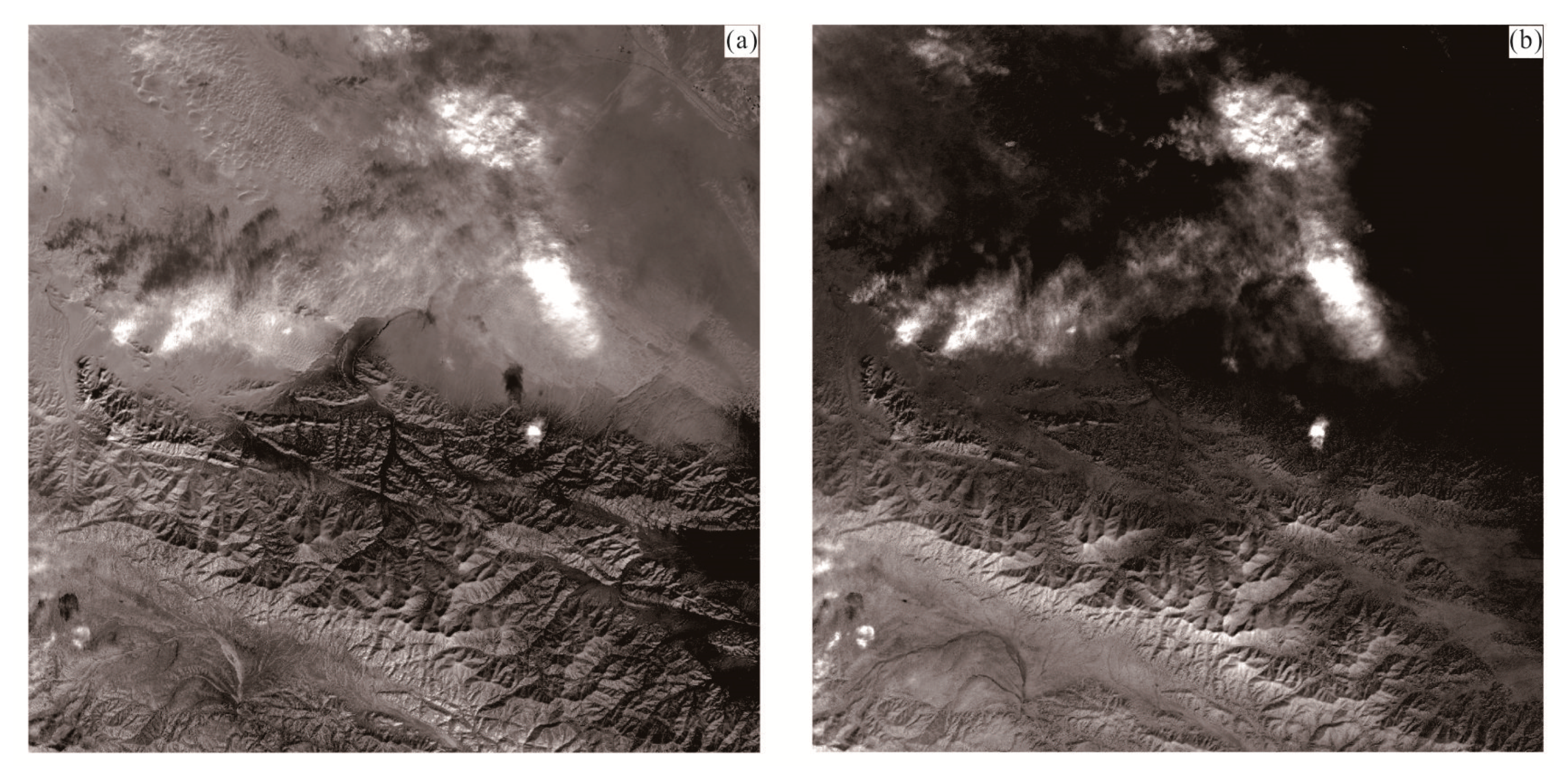
The end member spectra used for this classification were generated from an average of 4 pixels in total that surround the single point defining the training area. It produced more representative spectra than spectra based on a single pixel. Furthermore, the averaging process helped to produce spectra that were less noisy. The bright and dark areas on the DEM (slopes facing the sun-azimuth direction at the time of acquisition and the adjacent poorly illuminated back slopes) were avoided when possible. In order to maximize the band characteristics and avoid band information loss, we selected regions of interest (ROIs) ROI 1 and ROI 2 considering all the Sentinel-2 bands: ROI 1 depicts thin, mist-like clouds, and ROI 2 contains thick and thinner clouds as shown in Figure 2a. This is because thin cloud pixels are easily mixed with bare ground pixels, whereas thick clouds are often mistaken for snow and ice because of the spectral similarities. The procedure was implemented in the software MATLAB to obtain a new image with higher pixel values to represent the ROIs (target component). The results of the MF method are shown in Figure 3. Matched filter results are presented as grey-scale images with digital number MF values, the digital number values of MF image are normally distributed with a mean of zero, MF values of zero and lower represent the background (no target component), while pixels with higher MF values are considered to contain higher contents of the target component [41,42]. It is evident that Figure 3a reflects the presence of cloud and desert areas. Figure 3b indicates the presence of clouds as well as considerable snow anomalies. Given the normal distribution of the values of MF results, anomalies were determined using the DN-N fractal model.
2.3.2. Digital Number-Frequency (DN-N) fractal
The fractal concentration-area (C-A) algorithm is a state-of-the-art algorithm of the available unsupervised classification methods [43]. Remote sensing image consists of pixel arrays and a DN is assigned to each pixel, DN-A (C-A) fractal method addresses the power-law relation between the DN and the area (A) of the element content (DN) greater than a certain content threshold and is based on the spatial and geometric properties of the pixel value, pixel value frequency distribution, and image pattern. This method facilitates a visual representation of the variance of any given image. It can be expressed as follows:
where A (DN ≥ S) denotes the area occupied by pixels with DN values equal to and greater than a certain content threshold (S) [44]. The plot of ln(A) versus ln(DN) is usually multifractal and comprises a series of lines or segments and the fractal dimension B corresponds to the slope of each line. Each segment indicates a population (for example, a rock type) that is self-similar or self-affine for certain intervals of DN values; the upper and lower thresholds of the segment are used for image segmentation. Additionally, the “area” is the product of the pixel size and frequency (denoted N) of a certain DN threshold; thus, the “DN-A” schema is equivalent to and can be substituted for by the “DN-N” (namely, pixel value frequency) schema. Han et al. demonstrated its feasibility in remote sensing analysis [45].
We performed DN-N fractal processing on the MF values, and the details of the procedure and algorithm implemented in MATLAB are found in Zhao [46].
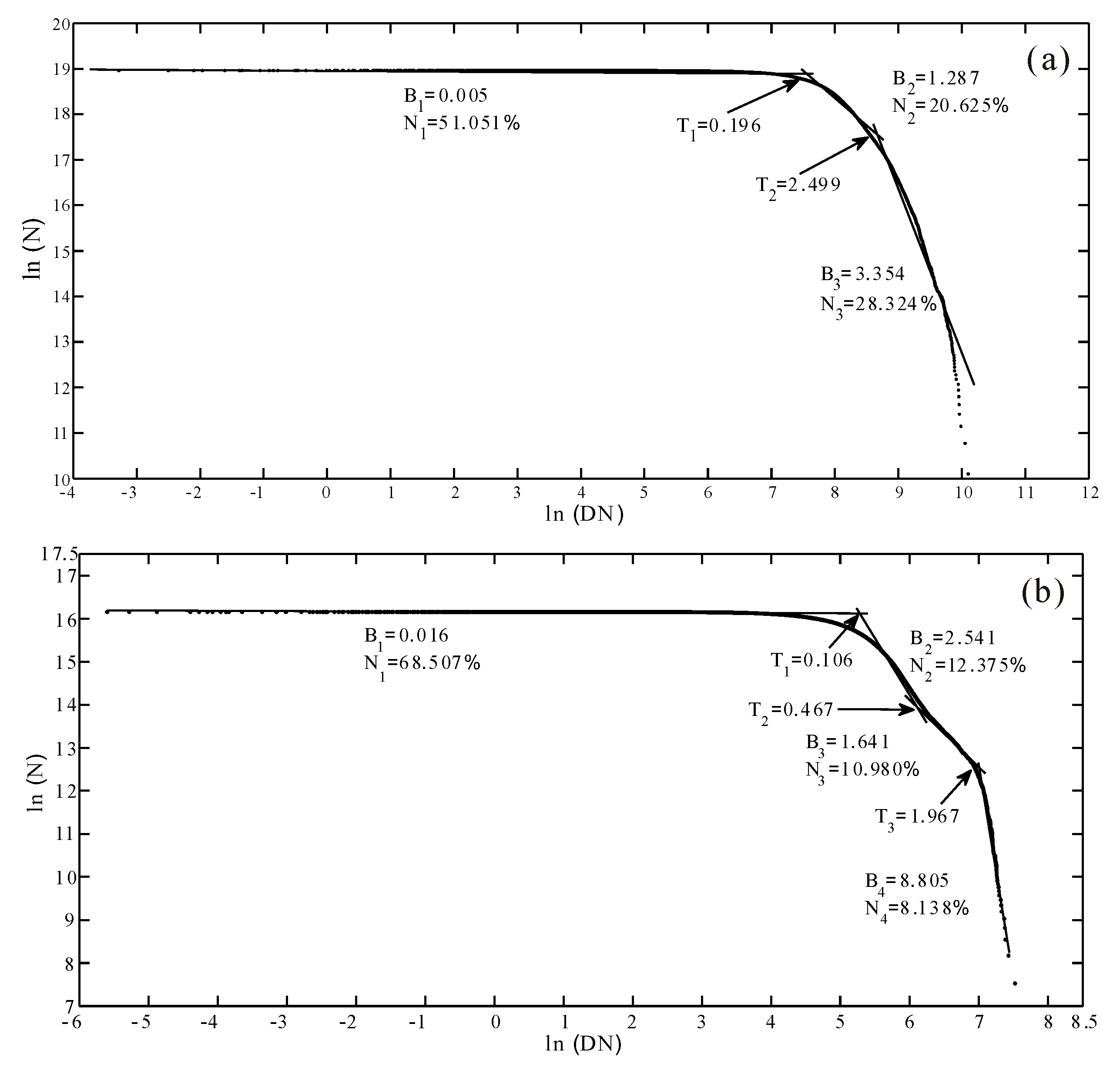
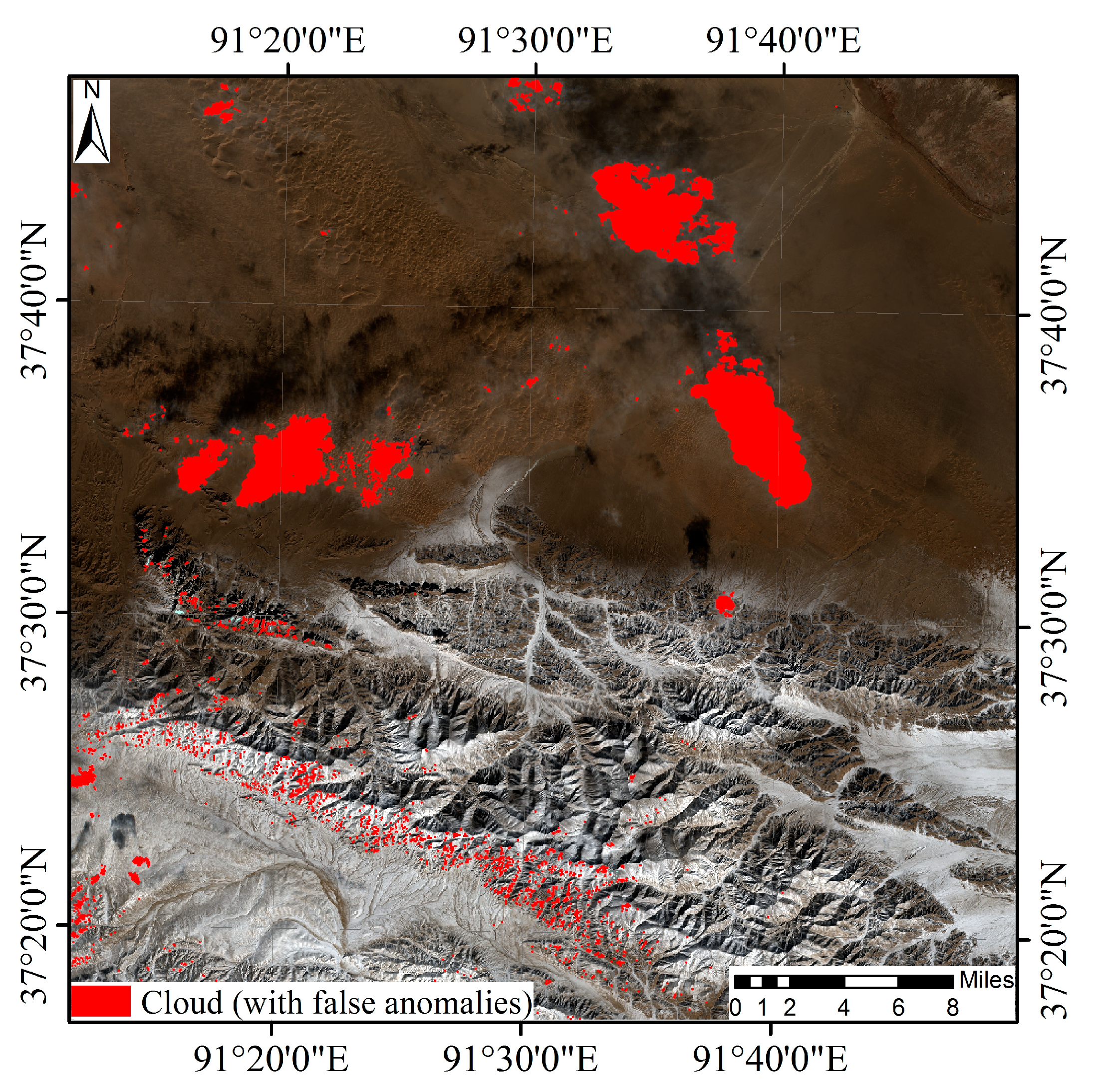
The non-scaling interval in Figure 4 corresponds to approximately one ground target. According to the results of the algorithm in the MATLAB, B2 and B3 in Figure 4a represent thin and thick clouds, respectively. The figure also includes many false anomalies related to snow and ice. In Figure 4b, B2, B3, and B4 indicate cloud areas, with B4 focusing on thick clouds. T1 = 0.106 is the lower limit of true anomalies. The threshold values of cloud were applied to ArcGIS 10.2 for visual assessment as shown in Figure 5. Most of the false anomalies are related to the snow and desert areas in the northeast.
When clouds are detected by the DN-N fractal model, as shown in Figure 5, the clouds and snow over different spatial distributions are classified in the same fractal (scale-less) range. This suggests that the extraction of certain anomalies cannot be achieved using pixel values alone. Clouds form clustered spatial structures, while snow is dispersed. Therefore, techniques such as fractal models, traditional density segmentation, and normal distributions cannot always detect clouds well. To address this problem, we explored the spatial analysis of anomaly patterns.
2.3.3. Spatial Analysis of Anomaly Patterns
(1) Anomaly-Overlaying Selection
Anomaly-overlaying selection was proposed by Liu et al. [47]. It was adopted in this study to eliminate the false anomalies caused by random interference while retaining real anomalies.
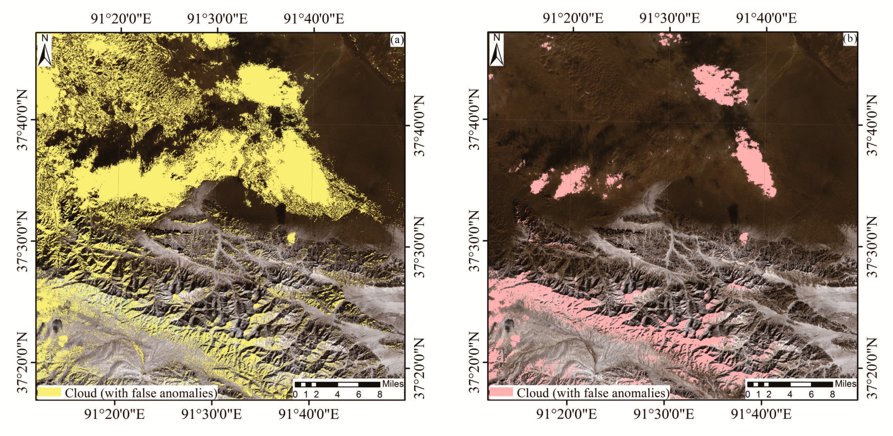
As Figure 5 shows, the results of the DN-N fractal model for ROI 1 and ROI 2 highlight information from different objects. Cloud cover (including thick and thin clouds) was detected in both cases. For ROI 1, the extraction results depict mainly clouds and bare land because of the spectral information selected, namely thin clouds mixed with bare land. For ROI 2, the main results of the extraction depict clouds and many false anomalies such as snow and ice. This is attributable mainly to the spectral similarities of thick clouds, ice, and snow. Thus, only a geographical information system (GIS)-based spatial anomaly-overlaying can identify false anomalies and provide accurate results.
The most remarkable characteristics of the resulting image (Figure 6) derived from the anomaly-overlaying are as follows: Most of the false anomalies are eliminated. Snow and ice anomalies with spectral features similar to those of clouds are mostly excluded. Most of the false anomalies containing bare land are also removed, thus providing a more accurate result. Some false anomaly patches are preserved, unexpectedly. However, unlike those in the ROI 1 and ROI 2 images, the remnants are less dominant.
In remote sensing, pixel values alone cannot be used to distinguish ground objects because false anomalies have spectral features similar to those of authentic anomalies. Anomaly-overlaying can eliminate most of the former, and the preserved anomalies have two notable features as shown in Figure 6. This feature is the degree of spatial clustering. A quantitative description of this characteristic benefits the identification process.
(2) Hotspot Analysis
The anomalies in Figure 6 exist as clustered or dispersed pixels or patches. The nature of clouds and snow/ice are such that the former can occur both in clusters and dispersions, while the latter scatters discontinuously. Thus, in this case, the degree of spatial clustering can plausibly act as a diagnostic distinction indicator to eliminate false anomalies, although both true and false anomalies frequently show similar or even identical spectral characteristics. In this study, a hotspot algorithm is adapted to measure the degree of clustering.
Hotspot and coldspot analysis can be used to illustrate the levels of spatial clustering of snow and cloud based on the Getis–Ord Gi statistic using ArcGIS 10.2 software [48]. Larger Gi scores correspond to higher attribute values in a given region; thus, a region in a high-value area generally has more spatial clustering. Details on this algorithm can be found in Yunus and Dou [49]. The Getis–Ord Gi statistic can be expressed using Equation (7), as follows:
where xj is the attribute value of feature j, wi,j is the spatial weight of elements i and j, n is the total number of sample points, is the mean value, and S is the standard deviation.
Our hotspot analysis findings can be summarized in two main points. Firstly, two types of patches representing clouds and snow/ice can be separated using their Gi scores. Generally, snow/ice has a significantly lower Gi score than cloud, even thin cloud cover. This confirms our assumption that cloud cover is integrated but snow/ice is not. Secondly, according to the range of cloud Gi scores, clouds can be divided further into thin, intermediate, and thick cover, with thick clouds having the largest Gi score.
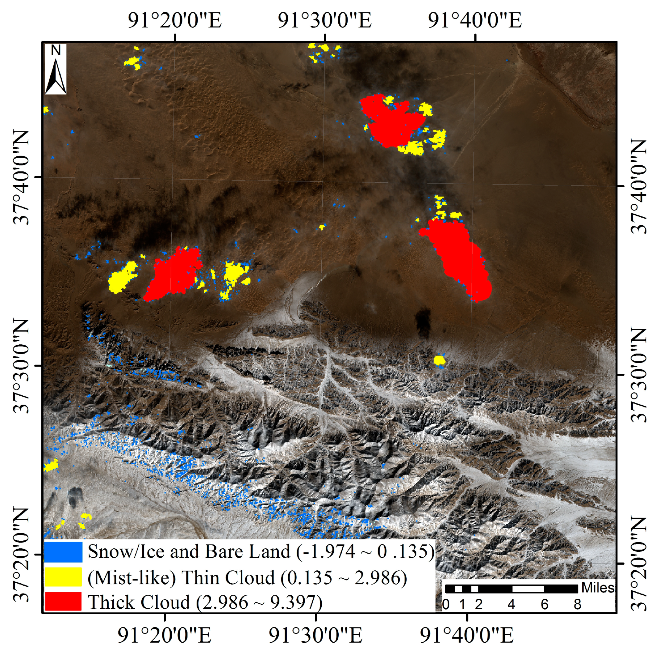
The clump operation results (with a 3 × 3 pixel moving window) conducted after the hotspot analysis are shown in Figure 7. This operation further enhances the original clustering or dispersing tendencies. Snow/ice, bare land, mist-like thin clouds, and thick clouds were detected.
3. Results and Discussion
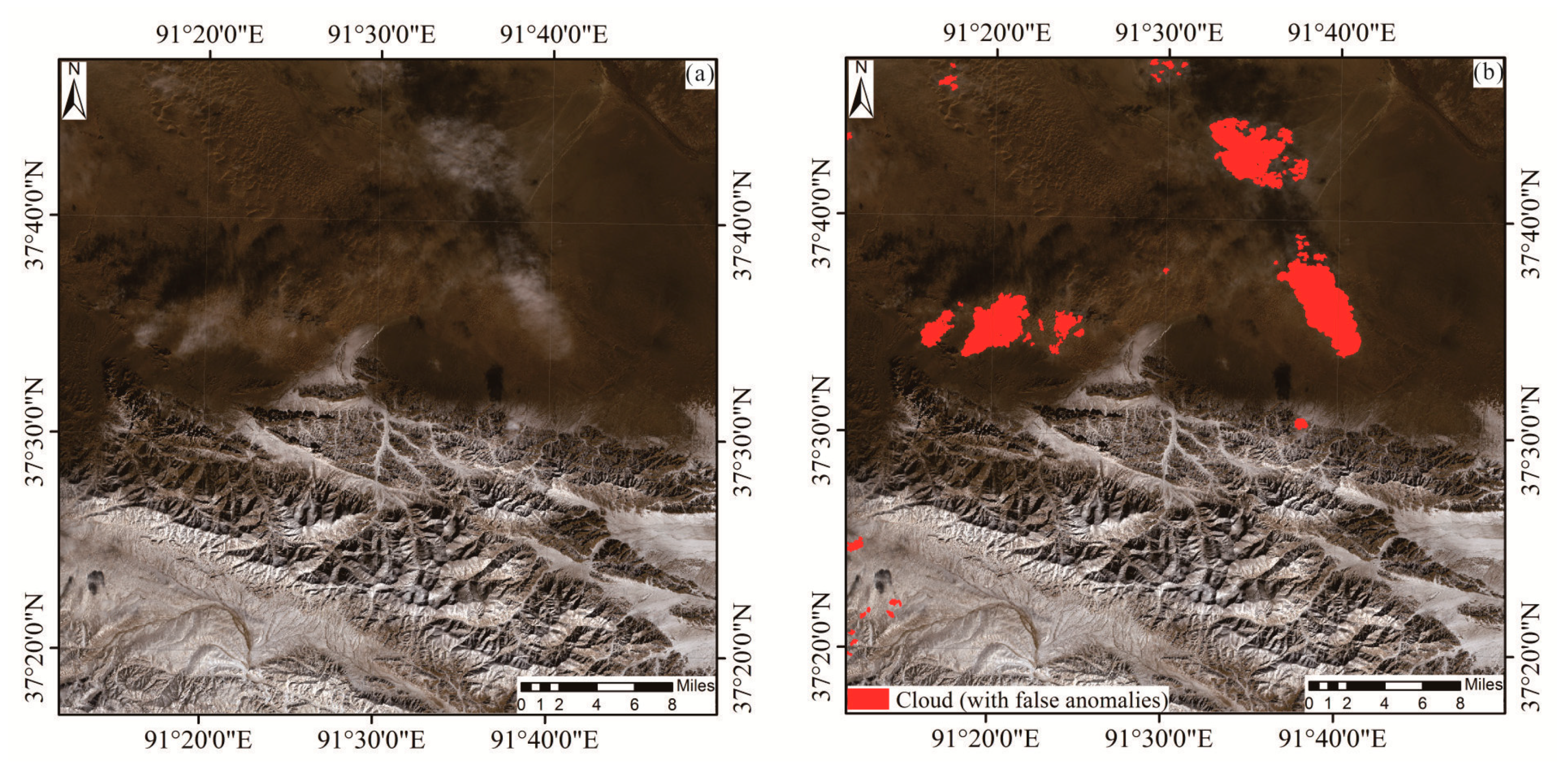
The DN-N fractal model produced false anomalies when it was used to process the curve of the MF image generated by ROI 1 and ROI 2, the detected features mainly had spectral characteristics similar to those of clouds, such as snow or desert regions, indicating that the pixel value alone cannot identify cloud regions. To account for this, we proposed a spatial point analysis, which was divided into steps of anomaly-overlaying analysis and hotspot analysis. The anomaly-overlaying analysis removed most false anomalies, because while both ROI 1 and ROI 2 can distinguish between thick and thin clouds, the main false anomalies indicated by both are different. Hotspot analysis avoided interference; although the false anomalies shared some spectral characteristics similar to those of clouds, the degree of spatial clustering could be used to eliminate the false anomalies. In Figure 8, the accuracy of the cloud detection data reached 97.017% with this technique.
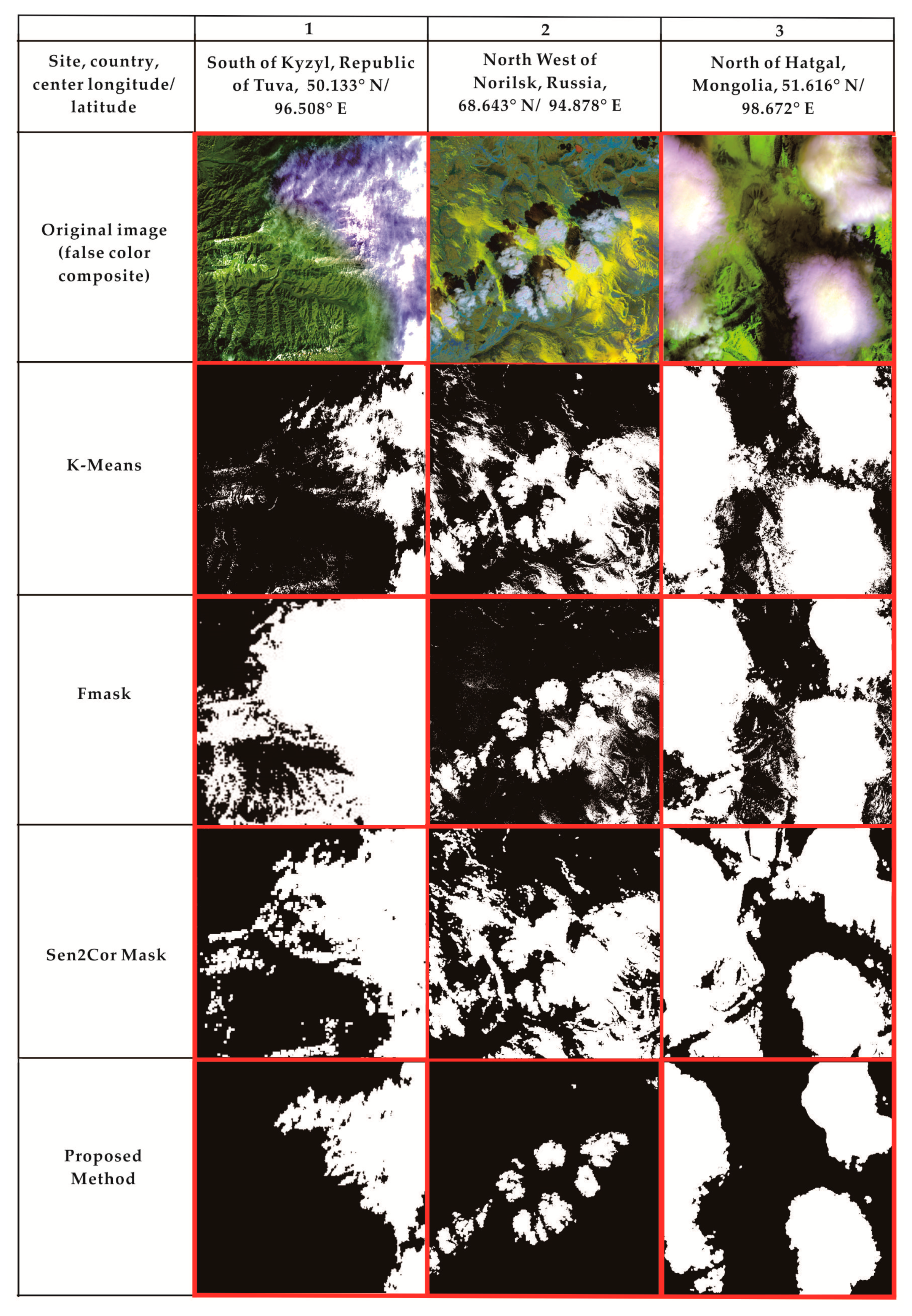
We selected a dataset acquired in different periods or times with snow and brightly colored ground objects on the underlying surface to test whether this approach can be used in more generic cases. To highlight the effects of cloud and snow separation, a representative experimental result was chosen to demonstrate the versatility of this algorithm. Feature areas were extracted from Sentinel-2 images including clouds, snow, and brightly colored ground objects. These results are shown in Figure 9.
The above figure compares the results of the proposed method of cloud detection against those obtained using classic methods, namely, the k-means, FMask and Sen2Cor methods. K-means algorithm [50] is a classical unsupervised classification algorithm. It is widely used in the remote sensing classification because of its simplicity and fast convergence [51,52]. FMask and Sen2Cor methods are advanced algorithms for cloud detection with Sentinel-2 images. FMask algorithm applied in this comparison is designed by Zhu et al. [11]. The result obtained by applying each application to our dataset is a binary mask: The white-colored areas represent clouds while black-colored areas represent features other than clouds. By comparison, all the classic methods appear to overestimate the amount of clouds as shown in Figure 9. This is because the spectral features of snow/ice and clouds in the images are very similar and high in reflectivity. Thus, clouds are easily confused with snow and ice. Table 1 quantifies the results of the three above-mentioned methods of cloud detection.
Three different accuracy assessments were used to assess the accuracy of the algorithm results [10]. The accuracy assessments are as follows (Equations (8)–(10)):
The manual mask (reference mask) was derived by a visual assessment of the full-resolution scene in Adobe Photoshop [10]. The result of the FMask algorithm and Sen2Cor method were better than traditional k-means method, but they still had a small amount of snow misjudged as cloud. The proposed method achieved high-precision cloud detection in areas where it is difficult to do so as shown in Table 1. The results of cloud detection using the extracted cloud-covered data indicated an overall accuracy exceeding 95%. The pixel values of clouds are high, similar to those for deserts and other brightly underlying surfaces. Consequently, salt-and-pepper noise causes researchers to mistake underlying surfaces for clouds. The method proposed in this study can be used to solve the problem of snow misclassification as cloud. Furthermore, this method eliminates the salt-and-pepper noise generated by brightly colored surfaces, thereby greatly improving the accuracy of cloud detection.
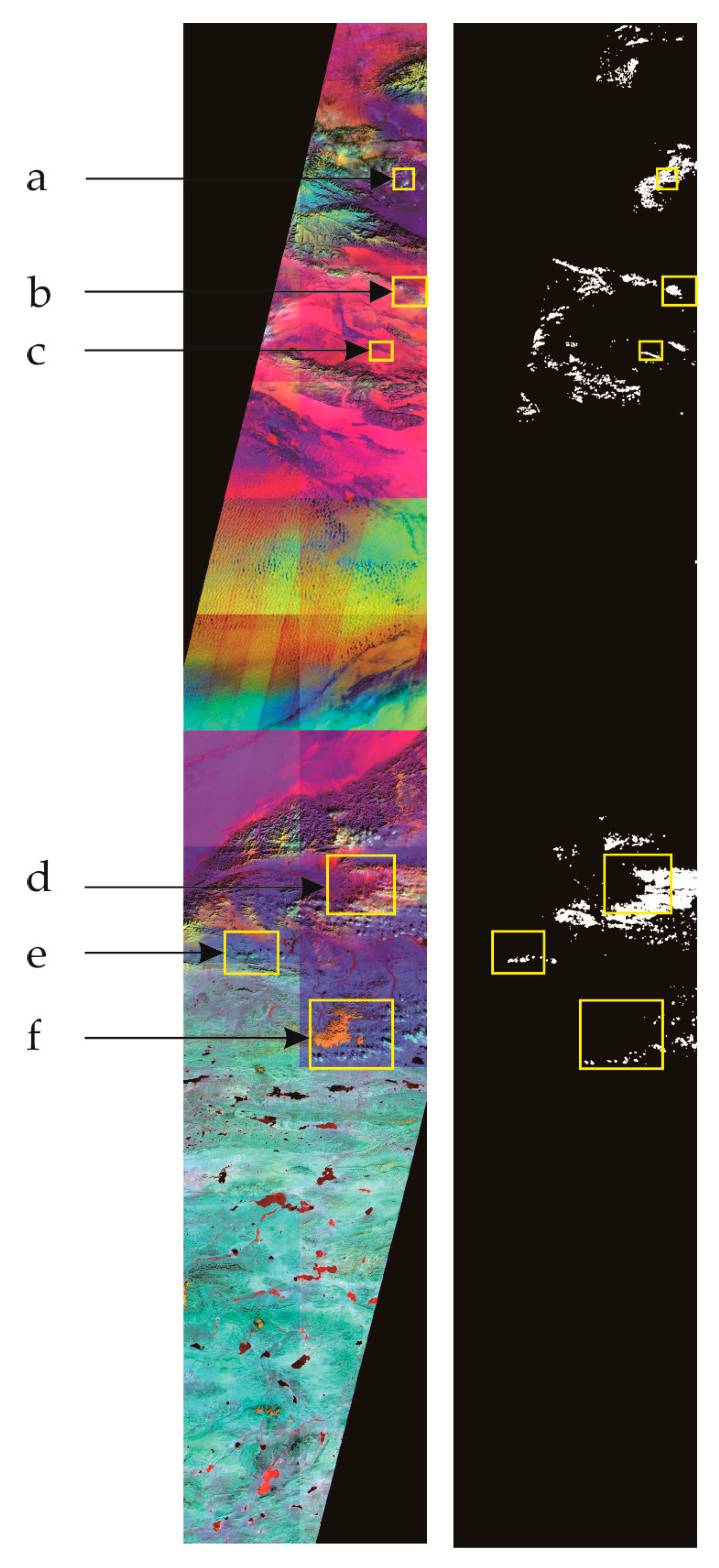
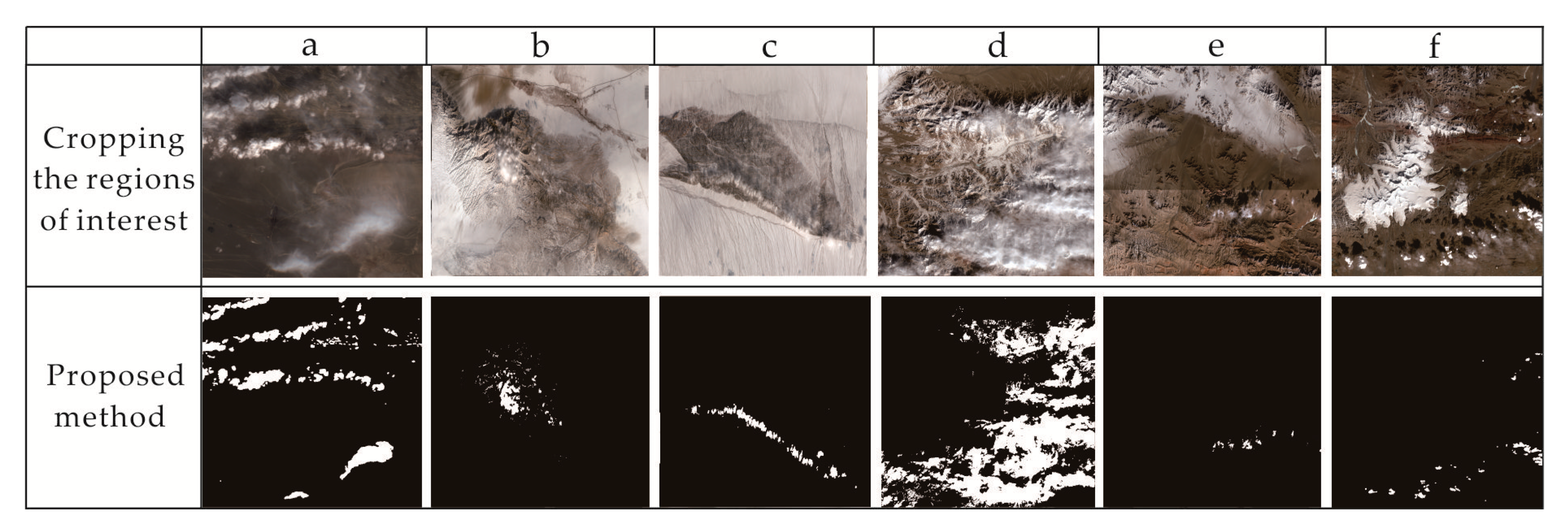
The result of a larger part dataset is shown in following Figure 10 and Figure 11. (Ingestion date: 31 January 2018, relative orbit number: 119, located in west China), six typical sites were selected as regions of interest. Figure 11 is an enlarged view of the indicated areas of detail shown in Figure 10. The results of cloud detection in the presence of a normal underlying surface were also found to be highly accurate (see inset to Figure 10a).
4. Conclusion
The study focused on a novel approach for cloud detection in areas with brightly colored ground objects. We compared the k-means, FMask and Sen2Cor methods for cloud detection to the proposed technique and concluded the following:
(1) According to our results, the DN-N fractal model performs better than the threshold method, but pixel values cannot distinguish one feature from another, because false anomalies share certain spectral features with authentic anomalies. Hence, we must consider another diagnostic characteristic, namely, clustering levels distribution.
(2) Most of the false anomalies containing bare land and snow/ice are removed by anomaly-overlaying. Some false anomaly patches are preserved, unexpectedly, but the remnants are less dominant; hotspot analysis can be used to determine locations where high or low values are spatially clustered. Misclassified snow and the underlying surface always show a more dispersed distribution than cloud does. Consequently, most false anomalies can be removed by clustering relationship analysis.
(3) The proposed method greatly reduced the misclassification of clouds and snow caused by the classic methods. It removed the salt-and-pepper noise caused by high DNs associated with deserts and other areas with similar features.
The proposed method is not limited by indefinable textures characters, complexity, and other factors; thus, it is versatile. However, cloud detection and accuracy assessment results for larger range images, such as global cloud cover, will be explored in future research.
Author Contributions
This research paper is completed by all authors. T.W. wrote the paper. L.H., T.W., Q.L., and Z.L. jointly developed the theoretical foundations.
Funding
This work was financially supported by the 1:50, 000 geological mapping in the loess covered region of the map sheets: Caobizhen (I48E008021), Liangting (I48E008022), Zhaoxian (I48E008023), Qianyang (I48E009021), Fengxiang (I48E009022), & Yaojiagou (I48E009023) in Shaanxi Province, China, under Grant [DD-20160060].
Conflicts of Interest
The authors declare no conflict of interest.
References
- Bunting, J.T.; d’Entremont, R.P. Improved cloud Detection Utilizing Defense Meteorological Satellite Program Near Infrared Measurements; Air Force Geophysics Lab Hanscom Afb Ma: Bedford, MA, USA, 1982. [Google Scholar]
- Dozier, J. Spectral signature of alpine snow cover from the landsat thematic mapper. Remote Sens. Environ. 1989, 28, 9–22. [Google Scholar] [CrossRef]
- Salomonson, V.V.; Appel, I. Estimating fractional snow cover from MODIS using the normalized difference snow index. Remote Sens. Environ. 2004, 89, 351–360. [Google Scholar] [CrossRef]
- Homan, J.W.; Luce, C.H.; McNamara, J.P.; Glenn, N.F. Improvement of distributed snowmelt energy balance modeling with MODIS-based NDSI-derived fractional snow-covered area data. Hydrol. Process. 2011, 25, 650–660. [Google Scholar] [CrossRef]
- Bertrand, C.; Gonzalez, L.; Ipe, A.; Clerbaux, N.; Dewitte, S. Improvement in the GERB short wave flux estimations over snow covered surfaces. Adv. Space Res. 2008, 41, 1894–1905. [Google Scholar] [CrossRef]
- Burtonjohnson, A.; Black, M.; Fretwell, P.T.; Kaluzagilbert, J. An automated methodology for differentiating rock from snow, clouds and sea in Antarctica from Landsat 8 imagery: A new rock outcrop map and area estimation for the entire Antarctic continent. Cryosphere 2016, 10, 1665–1677. [Google Scholar] [CrossRef]
- Beaudoin, L.; Nicolas, J.M.; Tupin, F.; Hueckel, M. Introducing Spatial Information in k-Means Algorithm for Cloud Detection in Optical Satellite Images. In Proceedings of the Europto Remote Sensing, Barcelona, Spain, 31 January 2001. [Google Scholar]
- Wang, W.; Song, W.G.; Liu, S.X.; Zhang, Y.; Zheng, H.Y. A Cloud Detection Algorithm for MODIS Images Combining Kmeans Clustering and Multi-Spectral Threshold Method. Spectrosc. Spectr. Anal. 2011, 31, 1061–1064. [Google Scholar]
- Le Hégarat-Mascle, S.; André, C. Use of Markov random fields for automatic cloud/shadow detection on high resolution optical images. ISPRS J. Photogramm. Remote Sens. 2009, 64, 351–366. [Google Scholar] [CrossRef]
- Zhu, Z.; Woodcock, C.E. Object-based cloud and cloud shadow detection in Landsat imagery. Remote Sens. Environ. 2012, 118, 83–94. [Google Scholar] [CrossRef]
- Zhu, Z.; Wang, S.; Woodcock, C.E. Improvement and expansion of the Fmask algorithm: Cloud, cloud shadow, and snow detection for Landsats 4–7, 8, and Sentinel 2 images. Remote Sens. Environ. 2015, 159, 269–277. [Google Scholar] [CrossRef]
- Candra, D.; Phinn, S.; Scarth, P. Cloud and cloud shadow masking using multi-temporal cloud masking algorithm in tropical environmental. Int. Arch. Photogramm. Remote Sens. Spat. Inf. Sci. 2016, 41. [Google Scholar] [CrossRef]
- Smith, A.; Wooster, M.; Powell, A.; Usher, D. Texture based feature extraction: Application to burn scar detection in Earth observation satellite sensor imagery. Int. J. Remote Sens. 2002, 23, 1733–1739. [Google Scholar] [CrossRef]
- Yu, W.; Cao, X.; Xu, L.; Mohamed, B. Automatic cloud detection for remote sensing image. Chin. J. Sci. Instrum. 2006, 27, 2184–2186. [Google Scholar] [CrossRef]
- Li, P.; Dong, L.; Xiao, H.; Xu, M. A cloud image detection method based on SVM vector machine. Neurocomputing 2015, 169, 34–42. [Google Scholar] [CrossRef]
- Vasquez, R.E.; Manian, V.B. Texture-based cloud detection in MODIS images. In Proceedings of the Remote Sensing of Clouds and the Atmosphere VII, Crete, Greece, 18 April 2003; pp. 259–268. [Google Scholar] [CrossRef]
- Zhu, L.; Xiao, P.; Feng, X.; Zhang, X.; Wang, Z.; Jiang, L. Support vector machine-based decision tree for snow cover extraction in mountain areas using high spatial resolution remote sensing image. J. Appl. Remote Sens. 2014, 8, 084698. [Google Scholar] [CrossRef]
- Racoviteanu, A.; Williams, M.W. Decision tree and texture analysis for mapping debris-covered glaciers in the Kangchenjunga area, Eastern Himalaya. Remote Sens. 2012, 4, 3078–3109. [Google Scholar] [CrossRef]
- Hughes, G. On the mean accuracy of statistical pattern recognizers. IEEE Trans. Inf. Theory 1968, 14, 55–63. [Google Scholar] [CrossRef]
- Bian, J.; Li, A.; Liu, Q.; Huang, C. Cloud and snow discrimination for CCD images of HJ-1A/B constellation based on spectral signature and spatio-temporal context. Remote Sens. 2016, 8, 31. [Google Scholar] [CrossRef]
- Müller-Wilm, U.; Devignot, O.; Pessiot, L. Sen2Cor Configuration and User Manual; ESA: Paris, France, 2016. [Google Scholar]
- Main-Knorn, M.; Pflug, B.; Louis, J.; Debaecker, V.; Müller-Wilm, U.; Gascon, F. Sen2Cor for Sentinel-2. In Proceedings of the Image and Signal Processing for Remote Sensing XXIII, Warsaw, Poland, 11–14 September 2017. [Google Scholar] [CrossRef]
- Kukawska, E.; Lewinski, S.; Krupinski, M.; Malinowski, R.; Nowakowski, A.; Rybicki, M.; Kotarba, A. Multitemporal Sentinel-2 data–remarks and observations. In Proceedings of the 2017 9th International Workshop on the Analysis of Multitemporal Remote Sensing Images (Multi-Temp), Brugge, Belgium, 27–29 June 2017. [Google Scholar] [CrossRef]
- Coluzzi, R.; Imbrenda, V.; Lanfredi, M.; Simoniello, T. A first assessment of the Sentinel-2 Level 1-C cloud mask product to support informed surface analyses. Remote Sens. Environ. 2018, 217, 426–443. [Google Scholar] [CrossRef]
- Van der Valk, D. Remote Sensing of Japanese WWII Airstrips in the Papua Province Republic of Indonesia; Delft University of Technology: Delft, The Netherlands, 2017. [Google Scholar]
- Roy, D.P.; Li, J.; Zhang, H.K.; Yan, L. Best practices for the reprojection and resampling of Sentinel-2 Multi Spectral Instrument Level 1C data. Remote Sens. Lett. 2016, 7, 1023–1032. [Google Scholar] [CrossRef] [Green Version]
- ESA (European Space Agency). Sentinel-2 User Handbook, Issue 1, Rev 2, Revision 2; ESA Standard Document; ESA: Paris, France, 24 July 2015. [Google Scholar]
- Crane, R.G.; Anderson, M.R. Satellite discrimination of snow/cloud surfaces. Int. J. Remote Sens. 1984, 5, 213–223. [Google Scholar] [CrossRef]
- Yokoya, N.; Chan, J.C.-W.; Segl, K. Potential of resolution-enhanced hyperspectral data for mineral mapping using simulated EnMAP and Sentinel-2 images. Remote Sens. 2016, 8, 172. [Google Scholar] [CrossRef]
- Strahler, A.H. The use of prior probabilities in maximum likelihood classification of remotely sensed data. Remote Sens. Environ. 1980, 10, 135–163. [Google Scholar] [CrossRef]
- Hogland, J.; Billor, N.; Anderson, N. Comparison of standard maximum likelihood classification and polytomous logistic regression used in remote sensing. Eur. J. Remote Sens. 2013, 46, 623–640. [Google Scholar] [CrossRef]
- Hutchison, K.D.; Cracknell, A.P. Visible Infrared Imager Radiometer Suite: A New Operational Cloud Imager; CRC Press: Boca Raton, FL, USA, 2016. [Google Scholar]
- Molan, Y.E.; Refahi, D.; Tarashti, A.H. Mineral mapping in the Maherabad area, eastern Iran, using the HyMap remote sensing data. Int. J. Appl. Earth Obs. Geoinf. 2014, 27, 117–127. [Google Scholar] [CrossRef]
- Oppenheim, A.V.; Lim, J.S. The importance of phase in signals. Proc. IEEE 1981, 69, 529–541. [Google Scholar] [CrossRef] [Green Version]
- Chen, Q.-s.; Defrise, M.; Deconinck, F. Symmetric phase-only matched filtering of Fourier-Mellin transforms for image registration and recognition. IEEE Trans. Pattern Anal. Mach. Intell. 1994, 1156–1168. [Google Scholar] [CrossRef]
- Harsanyi, J.C.; Chang, C.-I. Hyperspectral image classification and dimensionality reduction: An orthogonal subspace projection approach. IEEE Trans. Geosci. Remote Sens. 1994, 32, 779–785. [Google Scholar] [CrossRef]
- Ferrier, G. Application of imaging spectrometer data in identifying environmental pollution caused by mining at Rodaquilar, Spain. Remote Sens. Environ. 1999, 68, 125–137. [Google Scholar] [CrossRef]
- Boardman, J.W.; Kruse, F.A. Analysis of imaging spectrometer data using N-dimensional geometry and a mixture-tuned matched filtering approach. IEEE Trans. Geosci. Remote Sens. 2011, 49, 4138–4152. [Google Scholar] [CrossRef]
- Gan, F.P.; Wang, R.S.; Ai nai, M.A.; University, P. Beijing, Alteration Extracting Based on Spectral Match Filter(SMF). J. Image Gr. 2003. [Google Scholar] [CrossRef]
- Liu, Y.H.; Liu, S.F.; Zhang, C.; Pei, X.Y. The Weight Information Extraction of Clay Minerals Based on Hyperion Data: A Case Study of Ganzhou Area, Jiangxi Province. Remote Sens. Land Resour. 2010, 25, 26–30. [Google Scholar] [CrossRef]
- Williams, A.P.; Hunt, E.R., Jr. Estimation of leafy spurge cover from hyperspectral imagery using mixture tuned matched filtering. Remote Sens. Environ. 2002, 82, 446–456. [Google Scholar] [CrossRef]
- Han, L.; Zhao, B.; Wu, J.-J.; Wu, T.-T.; Feng, M. A new method for extraction of alteration information using the Landsat 8 imagery in a heavily vegetated and sediments-covered region: A case study from Zhejiang Province, E. China. Geol. J. 2018, 53, 33–43. [Google Scholar] [CrossRef]
- Cheng, Q.; Li, Q. A fractal concentration–area method for assigning a color palette for image representation. Comput. Geosci. 2002, 28, 567–575. [Google Scholar] [CrossRef]
- Shahriari, H.; Ranjbar, H. Image Segmentation for Hydrothermal Alteration Mapping Using PCA and Concentration–Area Fractal Model. Nat. Resour. Res. 2013, 22, 191–206. [Google Scholar] [CrossRef]
- Han, L.; Zhao, B.; Wu, J.J.; Zhang, S.Y.; Pilz, J.; Yang, F. An integrated approach for extraction of lithology information using the SPOT 6 imagery in a heavily Quaternary-covered region—North Baoji District of China. Geol. J. 2017. [Google Scholar] [CrossRef]
- Zhao, B.; Lei, Y.; Qiu, J.; Shi, C.; Zhang, D. Internal structural analysis of geochemical anomaly based on the content arrangement method: A case study of copper stream sediment survey in northwestern Zhejiang province. Geophys. Geochem. Explor. 2015, 39, 297–305. [Google Scholar]
- Liu, L.; Zhou, J.; Han, L.; Xu, X. Mineral mapping and ore prospecting using Landsat TM and Hyperion data, Wushitala, Xinjiang, northwestern China. Ore Geol. Rev. 2017, 81, 280–295. [Google Scholar] [CrossRef]
- Mitchel, A. The ESRI Guide to GIS analysis, Volume 2: Spartial measurements and statistics; ESRI Press: Redlands, CA, USA, 2005. [Google Scholar]
- Yunus, A.P.; Dou, J.; Sravanthi, N. Remote sensing of chlorophyll-a as a measure of red tide in Tokyo Bay using hotspot analysis. Remote Sens. Appl. Soc. Environ. 2015, 2, 11–25. [Google Scholar] [CrossRef]
- Arora, P.; Varshney, S. Analysis of k-means and k-medoids algorithm for big data. Procedia Comput. Sci. 2016, 78, 507–512. [Google Scholar] [CrossRef]
- Bruzzone, L.; Prieto, D.F. A technique for the selection of kernel-function parameters in RBF neural networks for classification of remote-sensing images. IEEE Trans. Geosci. Remote Sens. 1999, 37, 1179–1184. [Google Scholar] [CrossRef] [Green Version]
- Schowengerdt, R.A. Techniques for Image Processing and Classifications in Remote Sensing; Academic Press: Cambridge, MA, USA, 2012. [Google Scholar]
Figure 1.
Proposed method framework.

Figure 2.
High resolution Sentinel-2 images of the study area (cropping the region of interest, false color composite to help the reader visually differentiate between snow/ice and clouds [32]. Bands 4, 10, and 11 for Red, Green, and Blue, respectively), with the (a) original image, (b) cloud detection results using the traditional maximum-likelihood method.

Figure 3.
Results of the matched filtering (MF) method: (a) The MF result for ROI 1, and (b) the MF result for ROI 2.
Figure 3.
Results of the matched filtering (MF) method: (a) The MF result for ROI 1, and (b) the MF result for ROI 2.

Figure 4.
Fractal schema for ln(DN) versus ln(N) of (a) region of interest (ROI) 1 and (b) ROI 2; Bi (i = 1, 2, 3...) represents a fractal dimension of each segment, Ni (i = 1, 2, 3...) means the pixel size and frequency of a certain DN threshold, and Ti (i = 1, 2, 3...) represents the DN value.
Figure 4.
Fractal schema for ln(DN) versus ln(N) of (a) region of interest (ROI) 1 and (b) ROI 2; Bi (i = 1, 2, 3...) represents a fractal dimension of each segment, Ni (i = 1, 2, 3...) means the pixel size and frequency of a certain DN threshold, and Ti (i = 1, 2, 3...) represents the DN value.

Figure 5.
Cloud detection based on the DN-N fractal model. (a) Results of the DN-N fractal model for ROI 1, (b) results of the DN-N fractal model for ROI 2.
Figure 5.
Cloud detection based on the DN-N fractal model. (a) Results of the DN-N fractal model for ROI 1, (b) results of the DN-N fractal model for ROI 2.

Figure 6.
Output image of the anomaly-overlaying between ROI 1 and ROI 2.

Figure 7.
Output image of hotspot analysis based on the anomaly-overlaying between ROI 1 and ROI 2.

Figure 8.
Output image of cloud detection. Red colored areas represent clouds; a 100 m one-sided buffer zone around patches of thick cloud could include thinner clouds that were not detected previously. (a) Original image; (b) final cloud detection result.
Figure 8.
Output image of cloud detection. Red colored areas represent clouds; a 100 m one-sided buffer zone around patches of thick cloud could include thinner clouds that were not detected previously. (a) Original image; (b) final cloud detection result.

Figure 9.
Comparison of the proposed technique against other methods, using imageries in different areas (cropping the regions of interest).
Figure 9.
Comparison of the proposed technique against other methods, using imageries in different areas (cropping the regions of interest).

Figure 10.
Proposed method results of 25 Sentinel-2 scenes. Composited images with bands 4, 10, and 11 in red, green and blue, respectively, are shown on the left, and cloud masks are shown on the right with white color (cropping 6 regions of interest).
Figure 10.
Proposed method results of 25 Sentinel-2 scenes. Composited images with bands 4, 10, and 11 in red, green and blue, respectively, are shown on the left, and cloud masks are shown on the right with white color (cropping 6 regions of interest).

Figure 11.
Enlarged view of the six indicated areas of detail in Figure 10, (a–f) correspond to the six regions of interest in Figure 10.


Table 1.
Producer’s accuracy, user’s accuracy, and overall accuracy using the classic methods versus proposed method.
Table 1.
Producer’s accuracy, user’s accuracy, and overall accuracy using the classic methods versus proposed method.
| Algorithm | Producer’s Accuracy | User’s Accuracy | Overall Accuracy | |
|---|---|---|---|---|
| 1 | K-Means | 53.33% | 80.00% | 80.85% |
| FMask | 97.33% | 64.60% | 82.12% | |
| Sen2Cor | 94.67% | 78.02% | 89.79% | |
| Proposed | 96.00% | 96.06% | 97.45% | |
| 2 | K-Means | 92.01% | 47.92% | 77.02% |
| FMask | 90.06% | 75.37% | 91.49% | |
| Sen2Cor | 98.28% | 44.95% | 74.04% | |
| Proposed | 96.10% | 90.57% | 97.02% | |
| 3 | K-Means | 90.06% | 81.82% | 87.23% |
| FMask | 93.21% | 81.58% | 88.09% | |
| Sen2Cor | 95.46% | 73.08% | 82.98% | |
| Proposed | 93.06% | 96.90% | 95.48% |
© 2019 by the authors. Licensee MDPI, Basel, Switzerland. This article is an open access article distributed under the terms and conditions of the Creative Commons Attribution (CC BY) license (http://creativecommons.org/licenses/by/4.0/).
Share and Cite
MDPI and ACS Style
Han, L.; Wu, T.; Liu, Q.; Liu, Z. A Novel Approach for Cloud Detection in Scenes with Snow/Ice Using High Resolution Sentinel-2 Images. Atmosphere 2019, 10, 44. https://0-doi-org.brum.beds.ac.uk/10.3390/atmos10020044
AMA Style
Han L, Wu T, Liu Q, Liu Z. A Novel Approach for Cloud Detection in Scenes with Snow/Ice Using High Resolution Sentinel-2 Images. Atmosphere. 2019; 10(2):44. https://0-doi-org.brum.beds.ac.uk/10.3390/atmos10020044
Chicago/Turabian StyleHan, Ling, Tingting Wu, Qing Liu, and Zhiheng Liu. 2019. "A Novel Approach for Cloud Detection in Scenes with Snow/Ice Using High Resolution Sentinel-2 Images" Atmosphere 10, no. 2: 44. https://0-doi-org.brum.beds.ac.uk/10.3390/atmos10020044
Note that from the first issue of 2016, this journal uses article numbers instead of page numbers. See further details here.