Creating Truth Data to Quantify the Accuracy of Cloud Forecasts from Numerical Weather Prediction and Climate Models


1
Center for Space Research, The University of Texas at Austin, Austin, TX 78759, USA
2
Cloud Systems Research, Austin, TX 78748, USA
*
Author to whom correspondence should be addressed.
Atmosphere 2019, 10(4), 177; https://0-doi-org.brum.beds.ac.uk/10.3390/atmos10040177
Submission received: 15 February 2019
/
Revised: 27 March 2019
/
Accepted: 1 April 2019
/
Published: 3 April 2019
(This article belongs to the Special Issue Remote Sensing of Clouds)
Abstract
:Clouds are critical in mechanisms that impact climate sensitivity studies, air quality and solar energy forecasts, and a host of aerodrome flight and safety operations. However, cloud forecast accuracies are seldom described in performance statistics provided with most numerical weather prediction (NWP) and climate models. A possible explanation for this apparent omission involves the difficulty in developing cloud ground truth databases for the verification of large-scale numerical simulations. Therefore, the process of developing highly accurate cloud cover fraction truth data from manually generated cloud/no-cloud analyses of multispectral satellite imagery is the focus of this article. The procedures exploit the phenomenology to maximize cloud signatures in a variety of remotely sensed satellite spectral bands in order to create accurate binary cloud/no-cloud analyses. These manual analyses become cloud cover fraction truth after being mapped to the grids of the target datasets. The process is demonstrated by examining all clouds in a NAM dataset along with a 24 h WRF cloud forecast field generated from them. Quantitative comparisons with the cloud truth data for the case study show that clouds in the NAM data are under-specified while the WRF model greatly over-predicts them. It is concluded that highly accurate cloud cover truth data are valuable for assessing cloud model input and output datasets and their creation requires the collection of satellite imagery in a minimum set of spectral bands. It is advocated that these remote sensing requirements be considered for inclusion into the designs of future environmental satellite systems.
1. Introduction
The accuracies of cloud model predictions play critical roles in many real-time meteorological applications including air quality [1] and solar energy management [2] as well as a host of military and civilian aerodrome operations [3]. However, the verification of cloud model forecast performance can be challenging [4] and is seldom addressed by NWP (numerical weather prediction) and climate modelers. Thus, the WMO (World Meteorological Organization) has established methods for evaluating clouds and related parameters [5].
In an earlier publication, procedures that follow these WMO guidelines were presented to exploit remotely sensed satellite imagery and resultant cloud data products for quantitatively assessing water clouds in datasets commonly used in numerical weather prediction (NWP) and climate modeling [6]. That study focused on lower-level water clouds because they play a critical role in cloud feedbacks, which have been identified as the leading source of spread in estimates of climate sensitivity [7,8]. However, these procedures are equally valid for all cloud types as will be shown below. The procedures rely upon manually generated cloud/no-cloud (MGCNC) masks created from satellite imagery as a basis of establishing cloud cover fraction (CCf) truth or CCftruth data. In the application demonstrated, CCftruth was derived from multispectral imagery collected by the VIIRS (Visible Infrared Imager Radiometry Suite) sensor carried on the NASA/NOAA (National Aeronautics and Space Administration/National Oceanic and Atmospheric Administration) Suomi NPP (National Polar-orbiting Partnership) or S-NPP mission. These procedures have been applied to both re-analysis fields created from the North American Mesoscale (NAM) Forecast System and simulations generated with them using the WRF (Weather Research and Forecasting) model. In essence, VIIRS imagery and cloud data products derived from them are temporally and spatially collocated within NAM or WRF gridded fields to identify grid cells for comparison against the CCftruth data. VIIRS cloud phase products, quality controlled using color-composites of VIIRS imagery, can be to ensure only lower-level water clouds are considered in the match-up data sets. Comparisons between NAM CCf or CCfNAM and the CCftruth data, created from the VIIRS imagery, revealed a bias toward under-clouding in the NAM re-analysis data [6]. However, the bias shifts strongly toward overclouding in the WRF forecasts based upon these NAM data [9]. While the NAM cloud analysis data tended toward binary, i.e., gridded fields were mostly all cloud-free or completely cloudy, the WRF cloud forecast fields became even more highly binary even across large geographic areas which were observed to contain fields of small-scale stratocumulus in the satellite imagery. Furthermore, WRF was found in this case study to over-predict cloud cover fraction for lower-level water as well as higher-level clouds and frequently forecasts multiple cloud layers (at high and low altitudes) when only a single cloud layer was present. These results for lower-level water clouds are updated in the article to include all clouds.
The question might be logically asked, “How can accurate cloud cover truth measurements be created that support quantitative analyses of cloud model gridded forecast fields?” Obviously, the process to create such CCftruth data begins with the expert interpretation of clouds in temporal and spatial collocated multispectral satellite imagery. Then, the analyst performs a cloud/no-cloud analysis using one or more of the multispectral images and combines them into a manually generated cloud/no-cloud (MGCNC) mask, which is mapped to the model gridded cloud fields to form the CCftruth product, as discussed later in the article. First, in Section 2, the theoretical basis is presented for understanding qualitatively the cloud signatures in multispectral imagery, which is essential for creating accurate MGCNC analyses. Since the accuracy of the MGCNC masks depends upon the strength of the contrast between water and/or ice clouds and their surrounding backgrounds, a discussion of the spectral characteristics of the bands used to discriminate between these clouds and various background conditions is presented in Section 3. First, however, an overview is provided of the software used to create the MGCNC analyses along with results from earlier studies that validate the utility of these manual cloud analyses. Section 4 provides a discussion of the procedures used to map the MGCNC analyses into the projection of the gridded data to be evaluated and they are demonstrated in a new set of analysis for NAM and WRF cloud datasets. Conclusions are presented in Section 5.
The topics and information presented herein are derived from the experience and knowledge gained by the authors while generating MGCNC analyses that initially were used in the VIIRS sensor design process but ultimately became essential to the VIIRS cloud mask (VCM) calibration/validation project under the NASA/NOAA S-NPP program. (The VIIRS sensor is now carried on the operational U.S. polar-orbiting environmental satellite (POES) system.) It is the intent of the authors to offer our software and technical assistance to the larger, global cloud research community, with the hope that the community will facilitate the construction of large-scale, verification databases of cloud cover truth measurements, similar to those discussed in this presentation, and ultimately that those cloud cover truth databases will be made available to interested users and developers of NWP and climate models.
2. Theoretical Basis for Imagery Interpretation
A qualitative understanding of cloud signatures in multispectral imagery is essential for creating accurate MGCNC analyses; therefore, an overview is provided of key parameters influencing the signatures observed in the satellite imagery. The sensitivity of radiometers depends on the ratio of their internally generated signal to that produced by incoming radiation, i.e., signal-to-noise ratio or SNR. The optimal sensor design maximizes SNR in a cost-effective manner, e.g., increasing the size of the aperture, the field of view, and/or the bandwidth or improving detector performance [10]. The SNR specifications for the VIIRS reflective bands are found in Table 4.13 of Hutchison and Cracknell [11]. However, for simplicity, this discussion focuses on top-of-atmosphere (TOA) radiation independent of sensor characteristics since MGCNC analyses can be performed on imagery collected by any satellite sensor. Thus, consider the ability to manually identify a cloud in any given spectral band of imagery to be based upon the contrast between the cloud and the surrounding cloud-free background. This contrast is expressed by Equation (1) [11], assuming each pixel is either completely cloudy or completely cloud-free and noting that, while environmental satellite sensor designs use wavelength rather than wavenumber, this presentation stays with the latter to conform with Liou [12].
C = Iν(0)cloud /Iν(0)background
Depending upon the wavenumber (ν) of the radiation viewed in a given band, the TOA radiance at pressure equal zero, i.e., Iν(0), may be composed of reflected solar radiation, emitted thermal radiation, or both solar and thermal radiation when observations are made in the 3–5 µm wavelength interval under daytime conditions.
Again, for simplicity, consider the case of thermal (infrared) radiation as a narrow (monochromatic) beam of energy emitted from a surface through a cloud-free atmosphere to space. The monochromatic, upwelling infrared energy arriving from a cloud-free surface at the sensor is given by Equation (2) [12], where the first term on right hand side (RHS) is a direct transmission from the surface to the TOA, the second term is the upwelling atmospheric TOA radiation, and the third term is the downwelling atmospheric radiation reflect by the surface to the TOA:
where ν = wavenumber of emission;
| = Planck function at wavenumber (ν) for temperature (T) in K; | |
| = emissivity of surface at wavenumber (ν); | |
| = atmospheric transmittance between pressure level (ps) and space; | |
| = monochromatic radiance arriving at satellite; | |
| = surface pressure; | |
| s | = surface temperature. |
For imaging sensors, as opposed to sounders, the difference in atmospheric transmittance between adjoining pressure levels (p) is very small which makes the atmosphere, under cloud-free conditions, a secondary source of energy arriving at the sensor, as described in the integral terms in Equation (2). Thus, for the purpose of creating a manual cloud analysis, Equation (2) may be closely approximated by Equation (3), i.e., image quality is not impacted by ignoring energy contributions from atmospheric emissions.
Equation (3) [11] states that the vast majority of energy arriving at the satellite sensor, under cloud-free conditions, is dependent primarily upon only three primary components: the blackbody emission from the Earth’s surface, the emissivity of the surface, and the atmospheric transmission from the surface to the sensor. (A similar analysis would lead to another equation that represents the radiation arriving from the cloud top to the sensor.) The emissivity of a cloud may differ from its cloud-free background in some bi-spectral band combinations, thus improving the cloud-ground contrast [13,14]. However, in individual spectral bands, small temperature differences often occur between the cloud top and the background surface causing lower-contrast frequently between cloudy and cloud-free pixels in nighttime imagery. The lower the contrast, the more difficult it becomes to create a highly accurate MGCNC product from such imagery. In fact, MGCNC products can be very difficult to create under polar-nighttime conditions where cloud and surface temperatures may be extremely low and temperature differences are small. Therefore, again for simplicity, focus turns toward creating MGCNC products under daytime illumination conditions where contrasts can be larger between cloud pixels and cloud-free pixels for many background conditions.
For the case of solar radiation, the amount of TOA monochromatic energy reflected by a cloud-free Earth-atmosphere system into the sensor aperture is more complex and given for cloud-free conditions by Equation (4) [12]:
where
| = monochromatic radiance arriving at satellite; | |
| τ | = optical depth of each τ′ layer, while the atmosphere has a thickness of τ1; |
| Term A | = surface energy contribution attenuated to space; |
| Term B | = internal atmospheric contributions attenuated to space, sometimes referred to as path radiance [15]; |
| μ | = cosine of the angle between radiation stream and the local zenith angle; |
| ϕ | = azimuth angle. |
The complexity of this calculation lies in the source function term, , which is described for solar radiation as [12]
where
| Term C | = multiple scattering of diffuse (scattered) energy; |
| Term D | = single scattering of direct solar irradiance, F0; |
| ω | = single scattering albedo; |
| P(μ,φ;μ’,φ’) | = phase function; |
| F0 | = solar irradiance; |
| μ0 | = cosine of solar zenith angle; |
| φ0 | = solar azimuth angle. |
Again, a similar but more complex equation can be written to describe the amount of monochromatic TOA radiation arriving at the sensor under cloudy conditions. However, it should now be evident from the cloud-free condition that the contrast between a cloudy pixel and its cloud-free background at any wavelength across the solar spectrum depends upon differences in surface and cloud particle reflectance characteristics, the solar illumination present in the bandpass, the solar-Earth-sensor scattering geometry characteristics, and the atmospheric composition and scattering characteristic, e.g., particulate matter concentration. Thus, the obvious approach to maximize cloud versus cloud-free background contrast is to focus on spectral regions where the surface reflectance is low compared to the reflectance of clouds, as suggestion by Term A of Equation (4), and choose wavelengths, when possible, to minimize the path radiance effects described in Term B.
3. Creating Manually Generated Cloud Truth Data
It is possible to create highly accurate cloud truth data from the manually interpretation of satellite imagery [16]. Such analyses can be created by making a binary cloud/no-cloud (CNC) mask of a single spectral band, in simplistic scenes such as water clouds over ocean backgrounds, or from multiple bands of imagery when ice and water clouds exist over heterogeneous background conditions. The software used to make these manual analyses and the preferred spectral bands needed to construct them over different cloud and background conditions are discussed in the sections below. However, a correct understanding of the scene contents is the basis for creating an accurate truth analysis, and this understanding is typically facilitated through the use of false color composite images [17]. These color images are created by placing up to three spectral bands into a single RGB image. Bands are selected to exploit differences in cloud and surface reflectance characteristics as well as atmospheric transmittance in the bands, as will become more evident in the sub-sections that follow. False color composites provide a robust approach to accurately interpret all the features in most scenes, and the use of these composites, which may be composed of various band combinations, is a fundamental step in creating an accurate MGCNC analysis. Many examples of these composites with VIIRS-type imagery are shown by Hutchison and Cracknell [11].
3.1. Cloud Truth Software
Once the scene contents have been identified through the use of color composites, the binary CNC analysis is created in each important spectral band with unique software, i.e., the cloud truth software, which operates only on gray-scaled imagery. Important bands are those in which cloud signatures are maximized for each background type or viewing condition. The software does not support the use of color imagery. It does allow the analyst to segment the image and identify clouds in each sub-region of the image by making all pixels cloudy that have values that exceed a user-defined threshold. The cloud truth software then allows the analyst to combine the CNC analysis from each spectral band used in the analysis to form the final manual CNC analysis or MGCNC for the scene. This final analysis has also been called a merged CNC (MCNC) analysis.
The cloud truth software was designed over 25 years ago and written in the C-programming language. It was implemented in X-windows using the Motif graphics package on a DEC (Digital Equipment Corporation) Alpha workstation running the OSF (open software foundation) operating system. A complete description of the initial version of the software is available through the United States Patent Office [18]. More recently, the software has been migrated to Linux and runs under the Fedora 7, 8, and 9 operating systems on computers that have graphics cards that support the Motif versions used by these operating systems. The software is being evaluated for migration to more current versions of Linux and Motif and/or other graphics packages. It is hoped that this final package could be made available to the user community along with training on its use. An example of the application of this software, used to analyze a typical VIIRS imagery dataset, follows.
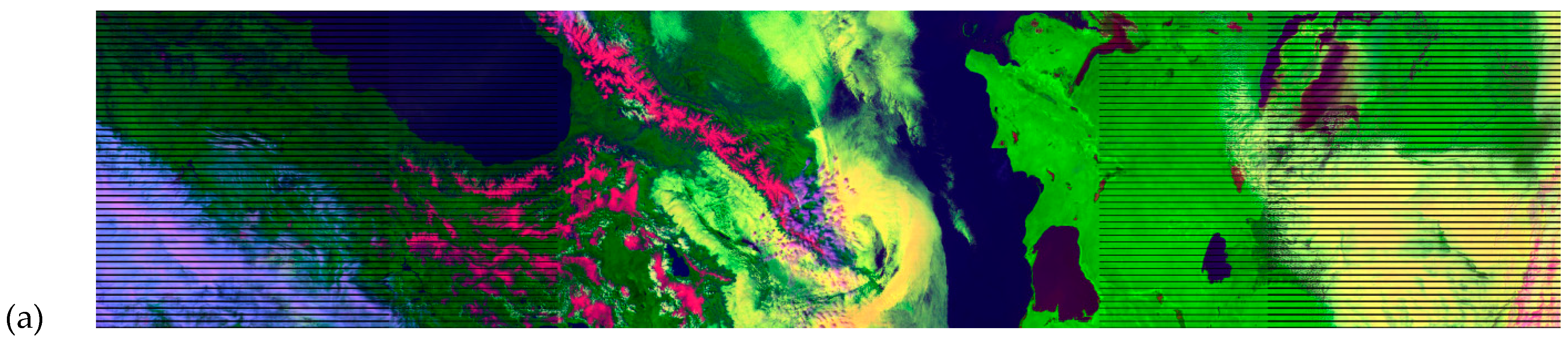
Figure 1a depicts clouds and surface features in a false color composite of a VIIRS moderate resolution granule centered on Azerbaijan and collected on 31 March 2013 at 0939 UTC. This moderate resolution VIIRS granule contains 3200 pixels in the cross-track direction and 768 pixels along the in-track direction of the satellites orbital path [11]. Both numbers are doubled for VIIRS imagery resolution data [11]. The color image, which is used only to help identify the scene contents, was created with Adobe Photoshop by assigning the VIIRS M1 (centered at 412 nm) band to red, the M10 (1610 nm) band to green, and the M16 (12,013 nm) band to blue in a red–green–blue (RGB) image. This particular RGB configuration was chosen to show snow/ice as red because the energy contribution from snow/ice is strong in the M1 band compare to the M10 and M16 bands. Densely vegetated surfaces appear dark green, since the strongest energy contribution comes from the M10 band while significant energy also comes from the M1 band. Sparsely vegetated (e.g., sand) surfaces appear light green because the strongest contribution is from the M10 while the M1 band contributes very little energy. Water clouds are yellow since they are highly reflective in the M1 and M10 bands but warm in the M16 band, while ice clouds have a purplish hue since the maximum energy contributions come from the M1 and M16 bands while the M10 band contributes much less energy. Since water has a low reflectance in both bands and is relatively warm, the Black Sea appears dark blue in the upper left while the Caspian Sea appears similarly in the center-right part of the image. The black horizontal lines on the left and right third of the scene do not represent missing data: they result from bow-tie deletion and the oversampling scheme used to ensure a VIIRS pixel growth of no more than 2:1 (e.g., 750–1500 m) in the cross-track direction [11]. The Garabogaz Aylagy of Turkmenistan is a pronounced feature along the eastern coastline of the Caspian Sea. A close inspection of the image reveals ice within many of the smaller lakes in Kazakhstan while extensive snow-covered areas are found in Caucasus Mountains located between the Black Sea and Caspian Sea. Cold dense ice clouds have a blue-purplish hue in the lower-left corner while potentially mixed phase clouds appear a lighter pink in the lower-right corner of the image. Note the ice clouds (purple) over the snow fields and lower-level water clouds in Eastern Azerbaijan.
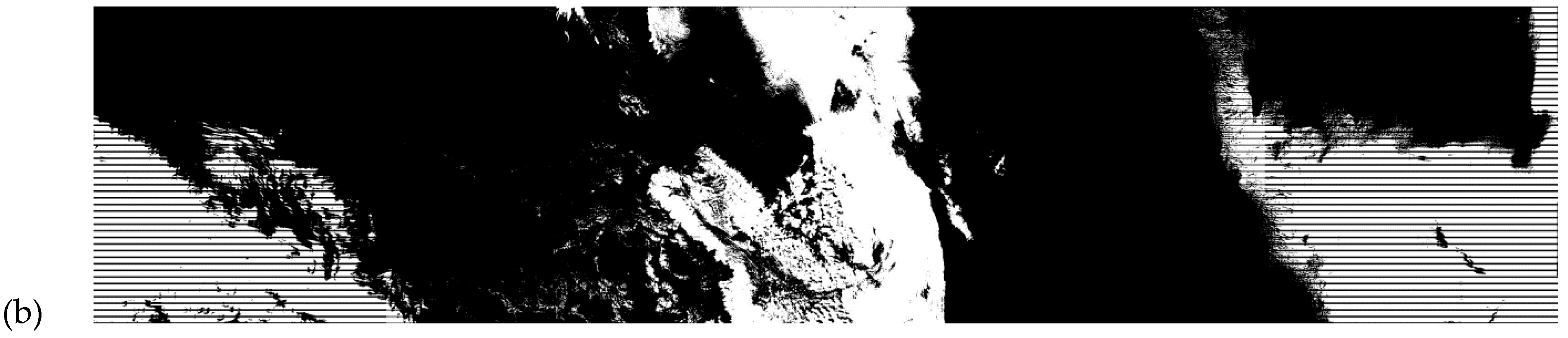
Figure 1b contains the MGCNC analysis that was created for this scene with the cloud truth software. This composited analysis was based upon the segmentation of the scene into different, near-homogeneous background conditions or regions using VIIRS imagery in the M1 (centered at 412 nm), M5 (672 nm), M9 (1378 nm), M10 (1610 nm), and M16 (12,013 nm) bands. The software allows the analyst to isolate clouds over a given region using the spectral band that provides the maximum contrast between the clouds and the background in order to create an accurate CNC image. Regions with different spectral characteristics are then analyzed with other VIIRS bands. The process is repeated until all cloudy pixels in the scene have been classified in one or more of the CNC images. There is no limit to the number of spectral bands that can be used with the software. In this case, five spectral bands were used to generate CNC images that were the composited into a final MGCNC analysis shown in the figure. This image segmentation process is briefly illustrated in Section 4.3.1 of Hutchison and Cracknell [11]. The basis for the segmentation process is discussed in the sub-sections that follow.
3.2. Evaluation and Validation of MGCNC Products
MGCNC products have been used successfully to establish and improve the performance of individual cloud detection tests [19], evaluate new spectral data to improve cloud detection algorithms [20], quantitatively assess the accuracy of operational cloud analysis and forecast models [21], and evaluate the accurate of clouds in datasets used in climate modeling [6]. However, only recently did the opportunity arise to validate these MGCNC analyses against another source of cloud truth data. That opportunity came during the NASA/NOAA S-NPP/JPSS VIIRS Cloud Mask (VCM) Algorithm Calibration Validation (Cal/Val) Project when VCM results derived from MGCNC analyses of global satellite imagery were compared to global cloud truth data collected by the NASA Cloud-Aerosol Lidar with Orthogonal Polarization (CALIOP) payload on the Cloud-Aerosol Lidar and Infrared Pathfinder Satellite Observation (CALIPSO) mission. The results from those analyses are summarized by Hutchison et al. [22] and Kopp et al. [23], and they are briefly highlighted here.
Special mention is made of the procedures followed during the development and use of the MGCNC analyses to ensure the integrity of the VCM Cal/Val Project. Prior to using any MGCNC analysis to quantify the performance of any VCM cloud product, the MGCNC analysis was first created by the corresponding author and then quality controlled (QC’d) by two additional subject matter experts (SMEs): Dr Andrew Heidinger (NOAA) and Dr Thomas Kopp (The Aerospace Corporation). This QC process was facilitated by the review of a presentation that contained color composites of the VIIRS imagery along with gray-scale images of the spectral bands used in creating the manually generated cloud analysis. The presentation also contained images of the cloud/no-cloud data. All images were co-registered. If any SME disagreed with the MGCNC analysis, in any region of the scene, the MGCNC analysis was re-examined until agreement was obtained between the SMEs. Experience showed that only rarely did an SME request a MGCNC analysis to be re-evaluated. Once all three SMEs agreed upon the accuracy of the MGCNC data, it remained unchanged and was used to evaluate the VCM cloud products for the duration of the Cal/Val project.
Two approaches were used to verify the VCM product performance under the Cal/Val program. One approach used 32 golden granules, consisting of 96 individual VIIRS granules with corresponding MGCNC analyses. The other approach used VIIRS matchups with CALIPSO data. Each golden granule consisted of 3-VIIRS granules, which is the minimum number of granules required to regenerate the operational results in an offline mode. Thus, there were 96 × 768 × 3200 (235,929,600) pixels in the MGCNC truth dataset. There were another 2,500,000 data points in the global CALIPSO-VIIRS matchup dataset. These match-ups were collected from the operational data stream of the S-NPP ground system and afforded no reprocessing capability to the VCM Cal/Val Project.
The primary VCM product performance metrics were probability of correct typing, false alarms, and leakage rates, which were generated from both truth data types. Overall, the performance of the VCM algorithm performance was found to be consistent with each source of truth data; however, the similarities in VCM performance using these two sets of cloud truth datasets was somewhat surprising [20] since the datasets did not cover identical times and locations. For example, PCT with the VCM algorithm during daytime conditions over ocean, land, and desert backgrounds, was 96.5%, 94.4%, and 95.7%, respectively, based upon the manually generated cloud truth data. Similar results obtained with CALIOP-VIIRS match-up data were 95.0%, 93.9%, and 96.0%, respectively. Additional comparisons between different conditions, e.g., nighttime and backgrounds, are available and show similar trends between these two sources of cloud truth data [22]. These comparisons help establish the validity of the MGCNC analyses. It was further concluded that the MGCNC and golden granules provide unique capabilities to quantitatively establish VCM algorithm performance across the entire 3200 km VIIRS data swath and to support the off-line simulations, i.e., reprocessing of VIIRS granules to evaluate potential solutions to VCM algorithm deficiencies prior to delivering code updates to the S-NPP ground station. This capability to support off-line simulations is considered critical to NWP and climate modeling activities. Finally, if such agreement is possible between two sources of cloud truth data at the VIIRS pixel level, surely errors in these truth data should be completely negligible when MGCNC analyses are converted to CCftruth data to evaluate cloud products from NWP and climate models run at much larger grid resolutions.
3.3. Phenomenology behind Feature Segmentation in Multispectral Imagery
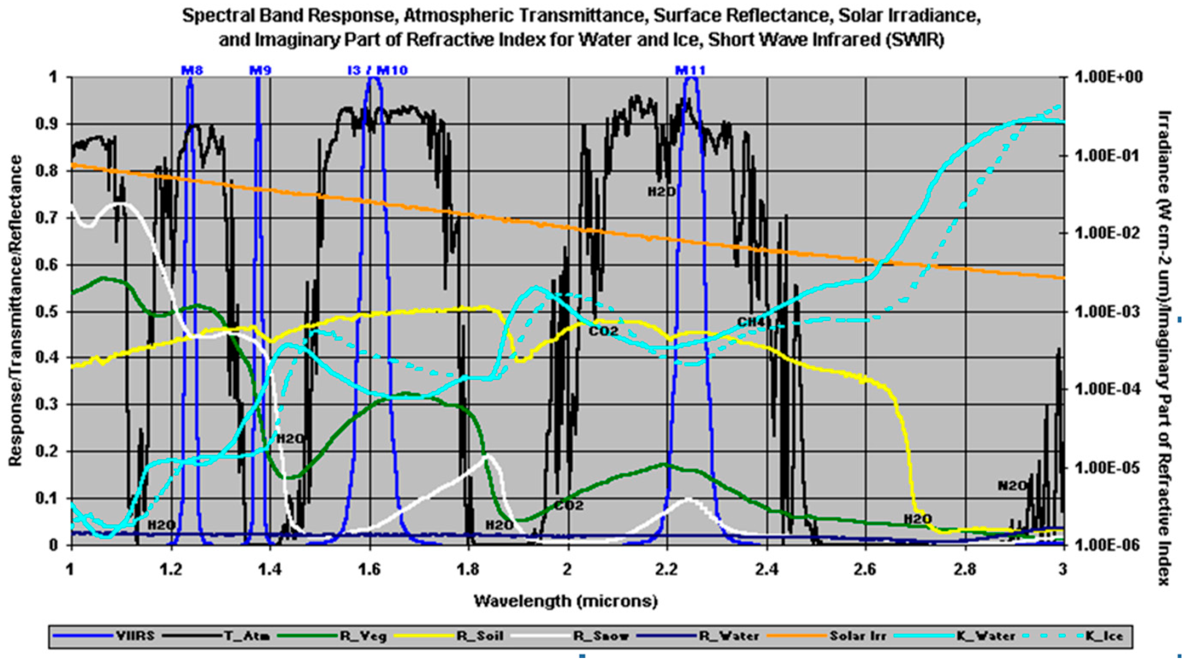
Figure 2 provides an overview of the phenomenology exploited in the image segmentation process in order to construct an MGCNC analysis. It contains the spectral signatures of cloud particles and surface backgrounds in 1.0–3.0 micron range. Similar figures are available in Baker (Figures 1–4) [24] and Hutchison and Cracknell (Figures 4.8–4.11) [11] for all VIIRS imagery (I) and radiometric (M) bands that collect energy from the near-UV to the IR bands, i.e., the 412–12,013 nm range.
Figure 2 is color coded as shown by the scale across the bottom of the image. The reflectivities of vegetated land (R_Veg) are shown in green, those of bare soil or sand (R_Soil) in yellow, those of snow (R_Snow) in white, and those of water or ocean (R_Water) in dark blue. Solar irradiance (Solar Irr) is orange, and atmospheric transmittance (T_Atm) is black. VIIRS band (i.e., M9, M10, I3) centers and widths are shown in medium blue lines with “M” labels at the top of the figure representing “moderate” resolution (750 m) bands as are the “I” imagery bands (i.e., I3) at 375 m resolution. Solid turquoise lines show the absorptive part of the index of refraction for water (K_Water) droplets, while dashed turquiose lines show that for ice particles (K_Ice).
Inspection of Figure 2 suggests that the contrast between water clouds, which are highly reflective in most VIIRS solar bands, and snow/ice would be strongest in the M10 band, where the reflectance of ice is nearly zero. The figure also shows that reflectances for many surfaces are in the 30–40% range for the M9 bandpass region, including snow/ice. The relatively high reflectances of these surfaces in the 1378 nm region were instrumental in the decision to reduce the VIIRS bandwidth in the M9 band to 15 nm [11], compared to the 30 nm bandwidth in MODIS (https://modis.gsfc.nasa.gov/about/specifications.php), in order to maximize the contrast between clouds and their background surfaces, especially under dry atmospheric conditions. Thus, based upon the expected improved contrast in the VIIRS M9 band, one should expect MGCNC analyses with VIIRS data to be more accurate than similar analyses performed with MODIS data as will be seen later in Figure 7.
3.3.1. Maximizing Cloud Contrast over Water Surfaces
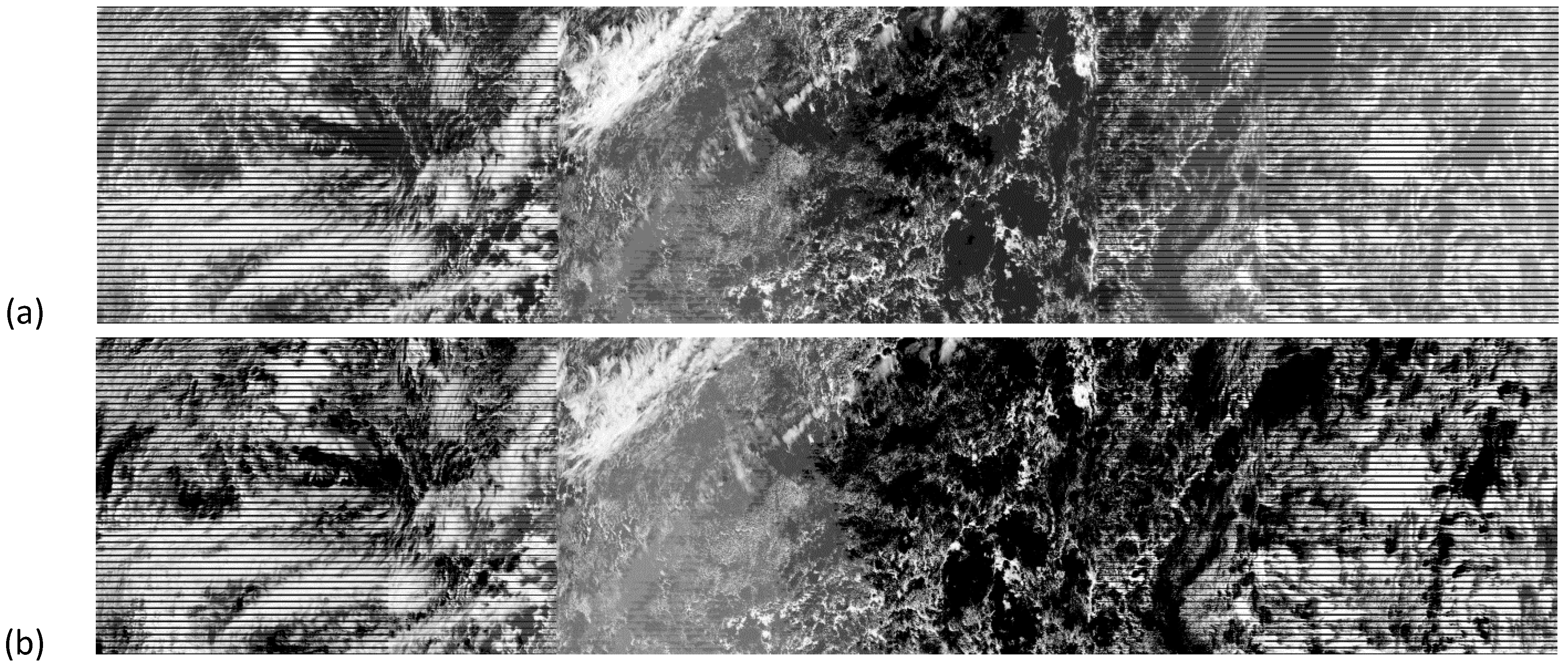
The reflectance of water is small across the entire solar spectrum; therefore, the contrast between clouds and the open ocean area is large at all these wavelengths. However, atmospheric scattering, i.e., path radiance, decreases as wavelength increases, so the maximum contrast occurs at wavelengths larger than those in the VIIRS M5 (672 nm) band. The impact of path radiance on cloud contrast is shown in Figure 3, which contains a VIIRS granule of a region of the North Atlantic Ocean at 1612 UTC on 20 Feb 2014. The cloud features in Figure 3a, i.e., showing the M5 band, appear blurred at both the edges of the scan and in the middle. The blurred appearance in the middle is due to sunglint and is unavoidable, i.e., it is due to the NPP orbit and is in the imagery of all solar bands. However, the blurring of features toward the scan edges is due to molecular scattering, which increases the path radiance toward the edges of the 3000 km VIIRS swath. This atmospheric scatter causes cloud versus background contrast to be reduced, thus cloud edges appear less distinct toward the edge of the scan. On the other hand, path radiance from molecular scattering is smaller in the M10 (1610 nm) band, seen in Figure 3b, so the cloud-background contrast remains stronger toward the edge of the swath. The difference in contrast is especially apparent when examining features in the right third of the image. Water cloud edges appear sharper and cloud-free areas are darker in the M10 band compared to the M5 band. Additionally, the M7 band (centered at 865 nm) is also useful to enhance the cloud-background contrast over ocean surfaces, especially in the presence of ice clouds since ice cloud edges may become less distinct in the M10 band as indicated by Figure 2.
3.3.2. Maximizing Cloud Contrast over Land Surfaces
While the surface reflectances of ocean surfaces are relatively constant at wavelengths across the solar spectrum, land reflectances vary greatly by wavelength and surface type. Consequently, several VIIRS bands are typically needed to construct accurate MGCNC analyses for ice and water clouds found over land backgrounds. For simplicity, however, this discussion is limited to major global surface types, i.e., densely vegetated land, coastal regions, sparsely vegetated land or bare soil (e.g., sand), and snow/ice covered surfaces.
Maximizing Cloud Contrast over Vegetated Land Surfaces
The reflectance of vegetated land is low (5–10%) in wavelengths shorter than the VIIRS M5 band (centered at 672 nm), as can be seen in Figure 4.8 of Hutchison and Cracknell [11] and Figure 1 of Baker [24]. It then begins to increase rapidly at about 700 nm and becomes over 50% at wavelengths in the 750–1000 nm range. The reflectance of vegetated land then drops at longer wavelengths but still remains over 50% in the VIIRS M8 band (centered at 1240 nm), ~28% in the M9 (1378 nm) band, ~30% in the M10 (1610 nm) band, and ~15% in the M11 (centered at 2250 nm) band. Therefore, the maximum cloud to background contrast over much of the global land surfaces is found in the M5 band where the surface reflectance and path radiance contributions to the total TOA radiance are minimal in the 400-700 nm range. The value of the M5 band for MGCNC analyses over vegetated land surface and many coastal regions is demonstrated in Figure 4.
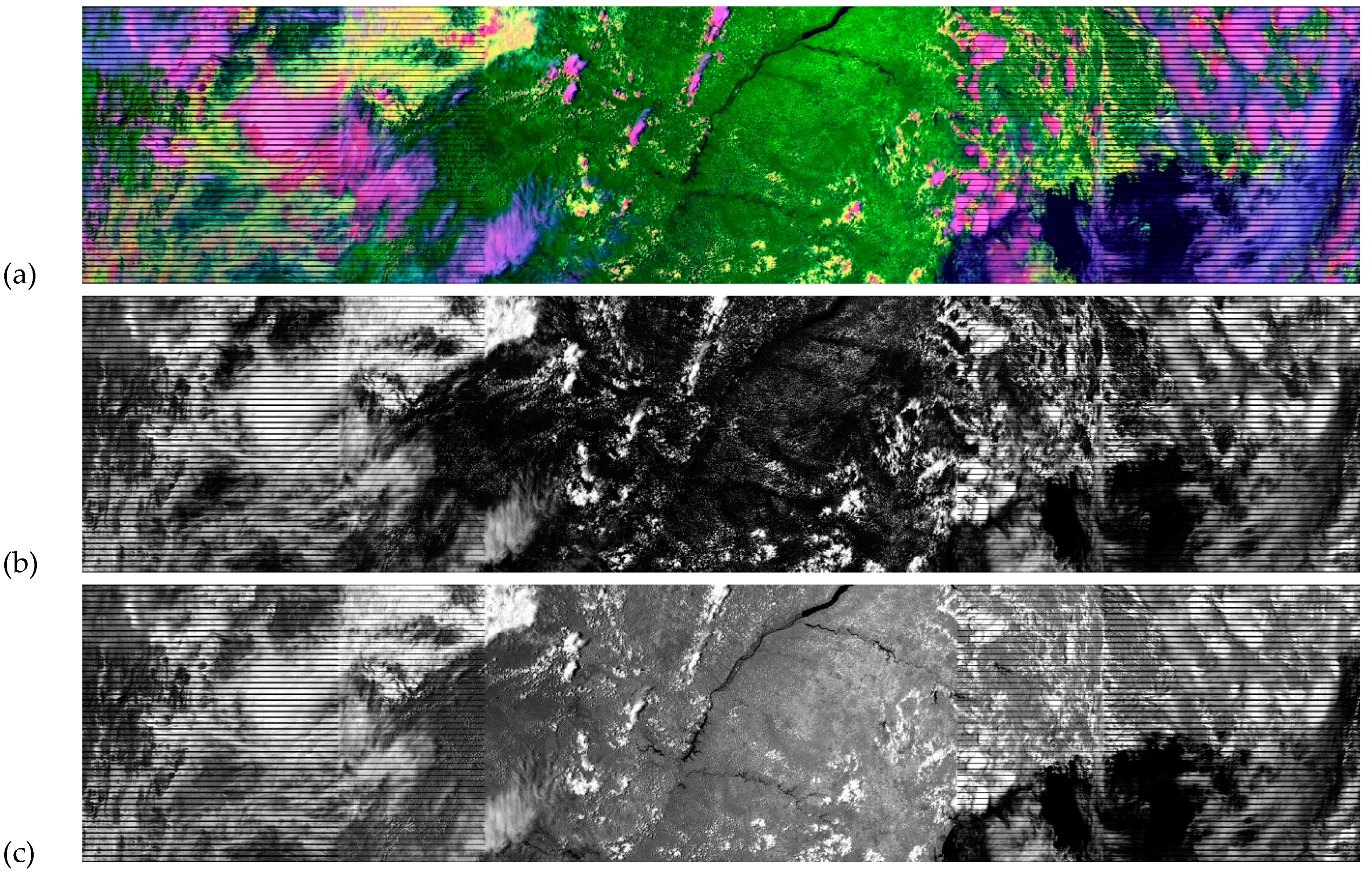
Figure 4a shows a false color composite of VIIRS imagery collected over South America on 17 January 2013 at 1714 UTC. The composite was created using the same band assignments in the RGB as described in Figure 1a. Therefore, vegetated surfaces appear dark green, water clouds are yellow, and thin ice clouds have a purplish hue while thicker ice clouds appear more pinkish. Ocean and water surfaces are dark.
Figure 4b shows the M5 band for this scene, and the absence of land and coastal features is obvious in this image. Clouds are evident along the river edges, which have distinct boundaries in the RGB image; however, only the absence of clouds suggests a coastline is present in the M5 image. On the other hand, the land, river boundaries, and coastlines boundaries are pronounced in the M7 (865 nm) band shown in Figure 4c. Thus, the M5 band is ideal for MGCNC analyses of water clouds over both vegetated land surfaces and most coastal regions.
Maximizing Cloud Contrast over Bare Soil Land and Desert Surfaces
Sparsely vegetated surfaces may include a variety of surfaces including desert and rock (mountain) regions. The MGCNC analysis for these desert-type surfaces typically exploits the relatively low reflectance of these surfaces in the near UV region of the solar energy spectrum. That makes the VIIRS M1 (412 nm) band most valuable, as seen in Figure 4.8 of Hutchison and Cracknell [11] or Figure 1 of Baker [24]. The reflectances of this surface type increase constantly from their minimum of ~5% at 400 nm to 25% at the M5 (672 nm) wavelength to nearly 50% at the M10 (1610 nm) wavelength. Thus, land and coastal regions in the M1 band appear similar to the features in the M5 band over vegetated land, as illustrated in Figure 5. However, atmospheric path radiance impacts the M1 band more severely than the M5 band; therefore, a radiance correction has been developed to reduce the effect of molecular scattering on features in this band [15]. It is emphasized that the VIIRS sensor design included M1 as a dual-gain band [11]. This allows M1 data to be used for cloud as well as ocean color analyses, without experiencing saturation as is commonly seen with similar MODIS imagery.
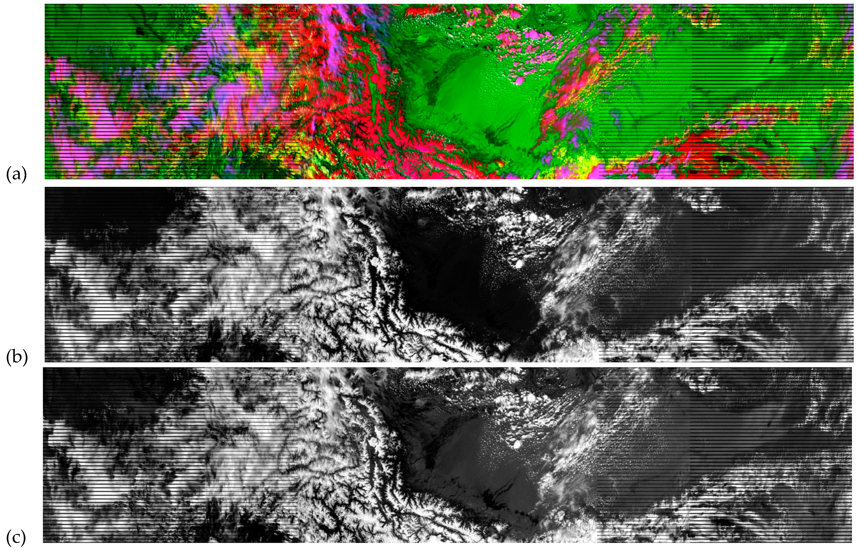
Figure 5a shows a false color composite of VIIRS imagery collected on 5 May 2012 at 0743 UTC over the Himalayan Mountains of Asia. Color assignments are as shown in Figure 1a and Figure 4a; water clouds are yellow, thinner ice clouds purple, thicker ice clouds pink, snow is red, and cloud-free land is green. The mostly cloud-free Taklamakan Desert appears green in the center of the image. Figure 5b contains the M1 image of the scene, while Figure 5c shows the scene in the M5 band. These images show that the contrast between cloud features and cloud-free land surfaces is stronger in the M1 band than in the M5 band, making the former critical in creating MGCNC analyses over bare soil and desert land surfaces.
Maximizing Cloud Contrast of Snow and Ice Surfaces
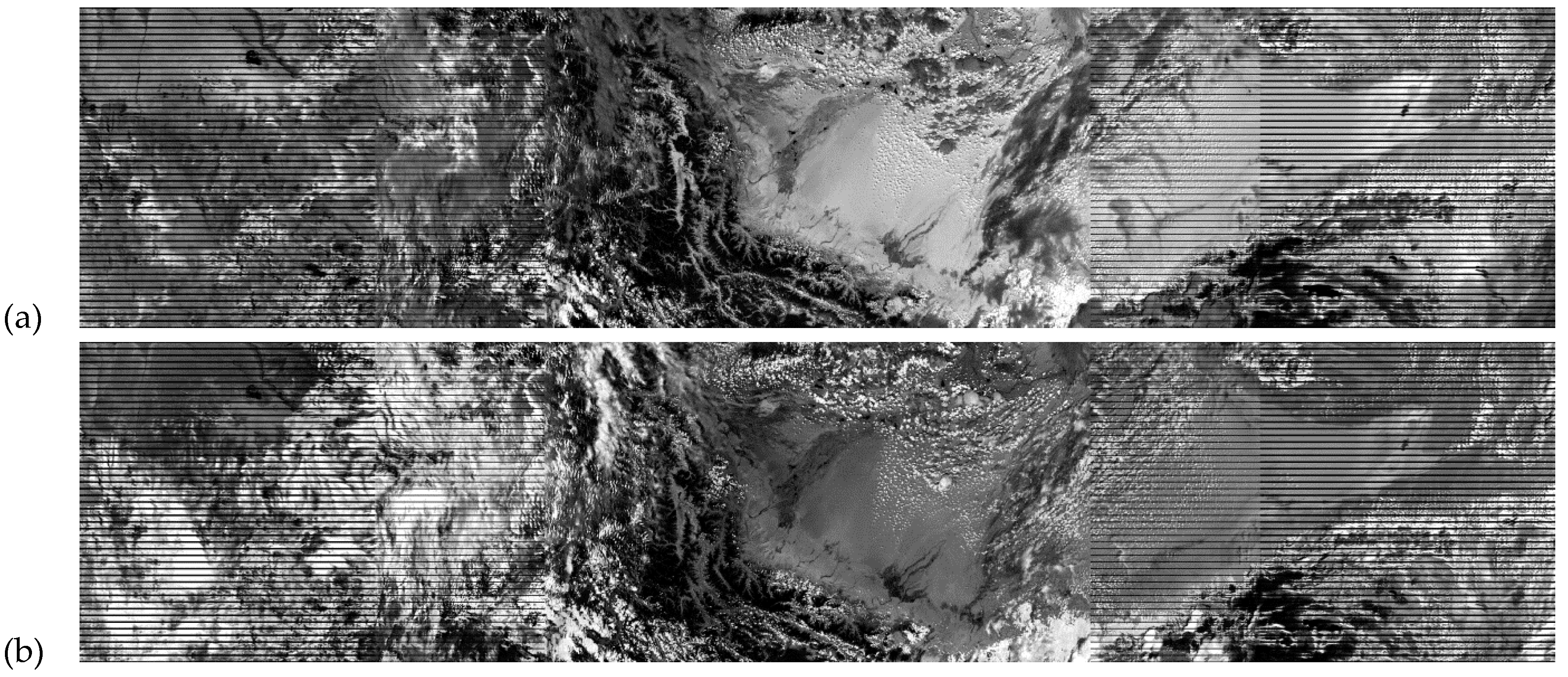
There are two options to maximize the contrast between snow/ice and clouds in VIIRS imagery and both are shown in Figure 6. One uses the conventional method of relying upon the VIIRS M10 (1610 nm) band shown in Figure 6a. However, a superior image exploits a brightness temperature difference (BTD) image created from the VIIRS M12 (centered at 3700 nm) band minus the M13 (centered at 4050 nm) band, i.e. creating a derived M12-M13 BTD image, and is shown in Figure 6b.
Snow appears black in both of these figures. In addition, the contrast between water cloud features surrounding the snow, shown by the dendritic pattern of Figure 5a, is strong in both images. However, the contrast between snow/ice surfaces and ice clouds is weak in the M10 band but much stronger in the BTD M12-M13 image as seen through the inspection of the left half of the scene. (Recall that ice clouds appear purplish in Figure 5a.) In addition, desert surfaces, such as the Taklamakan, are highly reflective in the M10 band but have a weaker signature in the BTD M12-M13 image, which provides improved contrast for detecting cloud fields in the upper right half of the scene. For more information on signatures in the BTD M12-M13 image, see [25].
Further Improving Cirrus Cloud Contrast over Snow/Ice Surfaces
Figure 6a,b indicate the potential challenge of creating MGCNC analyses in the presence of cirrus clouds, since these clouds can extend across a variety of surfaces that have diverse reflective characteristics, as seen in this scene. That challenge becomes even greater when cirrus clouds are found in vast snow/ice regions. Therefore, the preferred approach to create MGCNC analyses under cirrus cloudy regions employs a top-down technique, i.e., exploit VIIRS imagery in the M9 (1378 nm) band as a first step to identify higher-level ice clouds, then analyze the remaining lower-level water clouds using the other VIIRS bands discussed in the previous sections.
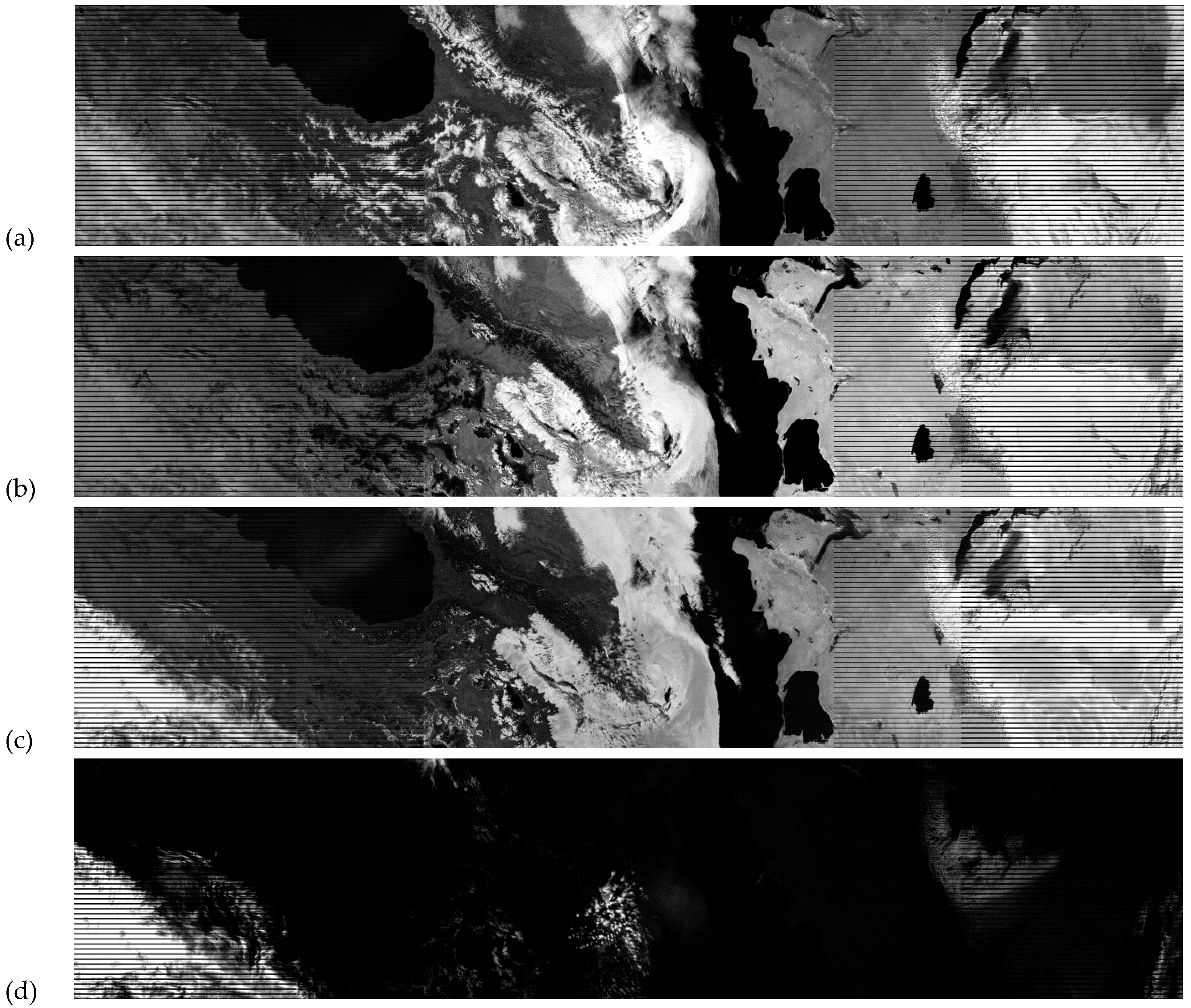
In Figure 7, attention returns to the VIIRS imagery collected on 31 March 2013 at 0939 UTC as shown in Figure 1. Figure 7a shows the M7 (865 nm) band. The large area of snow across the Caucasus Mountains is seen in the dendritic pattern in the left-middle part of the image. Cirrus clouds are indicated by the milky appearance in the left-lower part of the scene. The snow features turn dark in the VIIRS M10 (1610 nm) band shown in Figure 7b. In addition, the reflectance of the cirrus clouds is lower in this band, so the cloud edges in the lower-level corner become less distinct. On the other hand, in the BTD M12-M13 (3700–4050 nm) image shown in Figure 7c, the snow remains dark while the contrast around the cirrus cloud edges is enhanced in the BTD M12-M13 image.
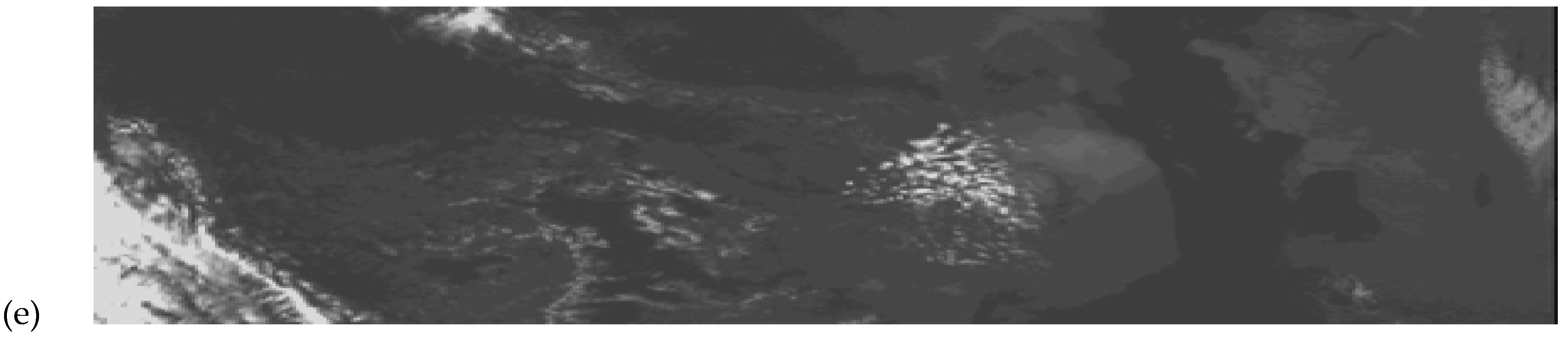
Finally, the contrast between middle and high altitude clouds is maximized in the VIIRS M9 band (with a bandwidth of 15 nm and centered at 1378 nm and shown in Figure 7d), while poorer contrast is seen in the corresponding MODIS band 26 (with a bandwidth of 30 nm and centered at 1375 nm) found at Figure 7e. (Note Figure 7d,e are not spatially or temporally collocated but are within about 20 min of each other in collection times.) In fact, the outline of the Caspian Sea is clearly visible in the MODIS image because the wings of this band extend into regions of relatively low atmospheric absorption as might be inferred from Figure 2. Thus, the surface reflectance is higher in the MODIS band, compared to the VIIRS M9 (1378 nm) band, so the contrast between clouds and the cloud free atmosphere is diminished in the MODIS band. Thus, to maximize the contrast between higher altitude clouds and all land surfaces, the VIIRS M9 band is the optimum band for exploitation. However, it is emphasized that the sensor bandpass should not exceed 15 nm in order to obtain the highest quality imagery with this band.
Therefore, to enable the accurate analysis of clouds in the scene shown in Figure 1, all VIIRS bands discussed above, i.e., M1 (412 nm), M5 (672 nm), M7 (865 nm), M9 (1378 nm), M10 (1610 nm), M12 (3700 nm), and M13 (4050 nm), provide essential information toward the generation of the MGCNC as shown in Figure 1b. Coupled with at least one longer-wavelength IR band, e.g., VIIRS M16 (12,013 nm) band, these 8 bands become the preferred combination of imagery data needed to create accurate MGCNC datasets under global daytime conditions. Again, to maximize the contrast between higher altitude clouds and all land surfaces, the 1378 nm band is the optimum band for exploitation. However, it is emphasized that the sensor bandpass should not exceed 15 nm in order to obtain the high quality imagery collected with the VIIRS M9 band.
4. Conversion of MGCNC Analyses into Truth Data
The pixel-level, binary MGCNC data, constructed using the phenomenology and procedures described in the previous sections, form the basis for creating the cloud cover fraction truth (CCftruth) data needed to quantitatively evaluate cloud model forecast performance. First, however, the MGCNC “pixel” satellite-based data must be mapped into the “cells” of a common grid with the cloud data generated by the model under investigation. Thus, the MGCNC pixel data becomes truth after it is temporally and spatially collocated with the gridded forecast cells on a user-defined grid, matched to the individual gridded data, and finally, aggregated to form the gridded data’s cloud/no-cloud truth.
A gross temporal collocation is introduced automatically through the selection of the satellite orbital path to coincide with the date and time of the gridded forecast fields. However, to guard against significant errors that might result from cloud motions in the satellite imagery, a more precise temporal constraint of +/− 30 min of the forecast verification time has been chosen. The temporal difference is readily computed by comparing the satellite sensor’s individual scan row times (for VIIRS, this information is found in the geolocation file) with the model forecast time. Truth pixels exceeding the model forecast time by the temporal constraint value are rejected.
For contiguous, equally spaced gridded data (i.e., there exists no gaps between adjacent cells of a constant resolution, and the data is found to be equally spaced in a specified projection), spatial collocation is accomplished by first establishing a grid where the gridded field geolocation forms the center of each cell. With the NAM data, for example, a grid with a resolution of 12.191 km is established when the data is projected into a Lambert Conformal Mapping. The satellite imagery geolocation, representing the MGCNC pixel center, is then projected into the same mapping and a simple interpolation is performed to determine the grid row and column number of the gridded field in which the MGCNC pixel is contained. MGCNC pixel centers outside the bounds of the gridded field are rejected. Each MGCNC pixel is furthered constrained to lie within a given radius of its matched gridded cell center. For earlier studies, an algorithm package implementing the Vincenty formulae was used to calculate the radial distances, and the radius was specified as 6.5 km [6]. Stricter constraints could be defined, if appropriate, to further ensure the full extent of the satellite imagery pixel is contained within the gridded cell, especially if the pixel resolution grows significantly with satellite scan angle. However, no more stricter constraint is necessary with VIIRS data, which grow to only 1.5 km at the edge of the VIIRS 3000 km swath from the nominal resolution of 750 m at nadir [11].
For non-contiguous, unequally spaced data (e.g., field data or where no mapping lends to an equally spaced gridded field), the spatial collocation step becomes complex and a more generalized approach must be followed. First a new grid must be defined at a resolution where no more than one sample data point is contained within the new cell. Both the conventional or modeled data and the satellite truth data are then mapped to this new grid. Because the conventional or modeled data are not guaranteed to be located at the center of the user-defined grid cells, a neighborhood of cells must be tested for nearby truth data. Note that, for the case of a user-defined equally spaced lat/lon grid (i.e., no projection into an alternative mapping) and a linear distance constraint, the pixel window defining the neighborhood changes due to the change in longitudinal distance with latitude (e.g., assuming a spherical earth, the longitudinal distance at 60 degree latitude is twice that at the equator). Investigations into this more generalized approach are being considered.
The collocation process yields a collection of truth data at the satellite pixel resolution for each gridded cell. Typically about 60–260 MGCNC pixels are matched to each NAM grid, depending upon the alignment of the VIIRS data within the grid. The CCftruth value for each gridded cell is then found by simply taking the average of the MGCNC binary pixel values within that grid. In addition, other satellite-derived cloud products can also be applied at this point. For example, a manually generated cloud phase analysis or an automated cloud phase product that has been quality-controlled with VIIRS imagery can be applied to restrict the analyses to water clouds alone as done in earlier studies [6].
To demonstrate the process of mapping MGCNC fields with cloud cover fraction (CCf), results were generated for a case study that analyzed NAM cloud fields and 24 h cloud forecasts based upon WRF simulations using them. The results, shown in Table 1, included all clouds in the NAM and WRF datasets. They are compiled from cases documented in two recent studies that focused only on lower-level water clouds [6,9].
Table 1 shows, at 10% CCftruth intervals (Column 1) and the performance metrics contained in Column 2, comparisons of CCfNAM data (Column 3) versus CCftruth (Column 4) valid for NAM data at 1800 UTC on 18 November 2014. Similar results for the WRF maximum CCf values found at all eta levels, determined as described by Hutchison et al. [9], at each collocated grid are shown in Column 5 along with the corresponding CCftruth (Column 6) for 1800 UTC on 19 November 2014. Since the CCf value from a single eta level is used to create these WRF statistics, the total CCfWRF values would be at least as large and more likely larger for multi-layered cloudy grids. It is emphasized that the results for the 24 h WRF forecasts shown in Table 1 are generated through the initialization of the same NAM data presented in this table, using WRF settings shown in Table 1 of Hutchison et al. [9].
The results in Table 1 show that the NAM mean CCf data are smaller than the CCftruth data, except for the near cloud-free truth bin, i.e., 0 ≤ CCftruth < 10 and 10 ≤ CCftruth < 20. The NAM mean values for the remaining bins range between about 10 and 50 percent lower than values contained in the CCftruth intervals. Therefore, in general, NAM under-specifies cloud cover contained in the satellite imagery. In addition, standard deviations are relatively large, e.g., 24–47 percent, which suggests that there appears to be a poor correlation between the CCftruth and model data.
Table 1 also shows that the WRF cloud forecast CCf fields are strongly binary in the 24 h forecast data with a strong tendency to over-predict clouds. Compared to CCftruth data, the CCfWRF mean values are greater than 80 percent at all CCftruth bins except the most cloud-free, i.e., 0 ≤ CCftruth < 10. In this bin, the CCfWRF mean value is 33.9 percent, while CCftruth is 0.8 percent. The large mean CCf values across all truth bins indicate that WRF cloud forecasts are much too large compared to truth data.
Therefore, the results shown in this case study suggests the CCfNAM fields are under-clouded compared to CCftruth while the resulting 24 h CCfWRF forecasts based upon these NAM data are much more binary and strongly over-clouded compared to the CCftruth. Analyses of additional case studies are needed to confirm these results; however, the ability to quantify the cloud cover fraction results of both input and output cloud fields greatly aids in the diagnosis of shortcomings found in these simulations. If these initial results are confirmed in additional studies containing larger datasets, a plan of action can be developed to better understanding the implications found in these NWP cloud analysis and forecast datasets pursuant to producing more reliable cloud forecast products.
5. Conclusions
Clouds are of critical importance to mechanisms that impact climate sensitivity studies as well as operational meteorological applications. However, the apparent difficulty in developing truth measurements for NWP and climate model cloud forecast verification results in an apparent omission in model performance statistics.
Therefore, a process of developing highly accurate cloud cover fraction truth data from manually generated cloud/no-cloud analyses of multispectral satellite imagery has been developed. The procedures to create the manually generated cloud analyses exploit the phenomenological features to maximize cloud signatures in a variety of remotely sensed satellite spectral bands to facilitate scene interpretation and create accurate cloud/no-cloud analyses. These MGCNC analyses have been used extensively to establish and improve the performance of individual cloud detection tests, evaluate new spectral data to improve cloud detection algorithms, and quantitatively assess the accuracy of operational cloud analysis and forecast models. However, the newer procedures discussed in this article collocate the MGCNC analyses with gridded cloud data to assess model cloud cover fraction (CCf) forecast performance of NWP and climate models. The process was demonstrated with NAM reanalysis fields and 24 h WRF cloud forecasts based upon these NAM data. The results showed strong over-clouding in the short-range WRF forecast, suggesting a potential issue in the conversion of WRF forecast variables into cloud cover fraction at the eta levels; however, further analyses of additional cases are needed before proceeding with the suggested plan of action.
It is concluded that highly accurate cloud cover truth data requires the collection of satellite imagery in a minimum set of spectral bands represented by the VIIRS bands M1 (412 nm), M5 (672 nm), M7 (865 nm), M9 (1378 nm), M10 (1610 nm), M12 (3700 nm), and M13 (4050 nm), and M16 (12,013 nm). In addition, it is emphasized that the design characteristics of the M1 band should be dual-gain, to eliminate saturation in cloudy conditions, and that the M9 bandpass should be restricted to no more than 15 nm, to ensure maximum contrast between cloud and surface features under dry atmospheric conditions.
Finally, it is recommended that the global cloud research community provide advocacy to ensure all future sensors provide cloud observations in these minimal set of spectral bands. Furthermore, this community should consider the construction of a large-scale, verification database of cloud cover truth measurements, similar to those discussed in this presentation, and develop an archival system to ensure those verification data sets are made available to interested users and developers of NWP and climate models.
Author Contributions
This article contains the results of research completed by both authors. K.D.H. is credited with the satellite imagery interpretation, the truth software, and MGCNC analyses; B.D.I. is credited with the collocation and processing results with the datasets.
Funding
This research received no external funding.
Acknowledgments
Data used in this study were obtained from the NCEP North American Mesoscale (NAM) 12 km Analysis, Research Data Archive at the National Center for Atmospheric Research, Computational and Information Systems Laboratory. http://rda.ucar.edu/datasets/ds609.0/.
Conflicts of Interest
The authors declare no conflict of interest.
References
- Pour-Biazar, A.; McNider, R.T.; Roselle, S.J.; Suggs, R.; Jedlovec, G.; Byun, D.W.; Kim, S.; Lin, C.J.; Ho, T.C.; Haines, S.; et al. Correcting photolysis rates on the basis of satellite observed clouds. J. Geophys. Res. Atmos. 2007, 112, D10302. [Google Scholar] [CrossRef]
- Mathiesen, P.J.; Collier, C.; Kleissl, J.P. Development and validation of an operational, cloud-assimilating numerical weather prediction model for solar irradiance Forecasting. In Proceedings of the ASME 2012 6th International Conference on Energy Sustainability, San Diego, CA, USA, 23–26 July 2012; pp. 955–964. [Google Scholar] [CrossRef]
- Fitch, K.E.; Hutchison, K.D.; Bartlett, K.S.; Wacker, R.S.; Gross, K.C. Assessing VIIRS cloud base height products with data collected at the Department of Energy Atmospheric Radiation Measurement sites. Int. J. Remote Sens. 2016, 37, 2604–2620. [Google Scholar] [CrossRef]
- Jakob, C.; Pincus, R.; Hannay, C.; Xu, K.-M. The use of cloud radar observations for model evaluation: A probabilistic approach. J. Geophys. Res. 2004, 109, D03202. [Google Scholar] [CrossRef]
- World Meteorological Organization (WMO). Recommended Methods for Evaluating Clouds and Related Parameters. In World Weather Research Program (WWRP); WWRP 2012-1; World Meteorological Organization (WMO): Geneva, Switzerland, 2012; p. 34. Available online: http://www.wmo.int/pages/prog/arep/wwrp/new/documents/WWRP_2012_1_web.pdf (accessed on 20 December 2018).
- Hutchison, K.D.; Iisager, B.D.; Jiang, X. Quantitatively assessing cloud cover fraction in numerical weather prediction and climate models. Remote Sens. Lett. 2017, 8, 723–732. [Google Scholar] [CrossRef]
- Bader, D.; Covey, C.; Gutowski, W.; Held, I.; Kunkel, K. Climate Models: An Assessment of Strengths and Limitations. US Dep Energy, Paper 8. 2008. Available online: http://digitalcommons.unl.edu/usdoepub/8 (accessed on 20 December 2016).
- Bony, S.; Colman, R.; Kattsov, V.M.; Allan, R.P.; Bretherton, C.S.; Dufresne, J.-L.; Hall, A.; Hallegatte, S.; Holland, M.M.; Ingram, W.; et al. How well do we understand and evaluate climate change feedback processes? J. Clim. 2006, 19, 3446–3482. [Google Scholar] [CrossRef]
- Hutchison, K.D.; Iisager, B.D.; Sudhakar, D.; Jiang, X.; Quaas, J.; Markwardt, R. Evaluating WRF cloud forecasts with VIIRS imagery and derived cloud products. Int. J. Remote Sens. 2019, in press. [Google Scholar]
- Stewart, R.H. Methods of Satellite Oceanography; University of California Press: Berkeley, CA, USA, 1985; p. 360. [Google Scholar]
- Hutchison, K.D.; Cracknell, A.P. VIIRS—A New Operational Cloud Imager; CRC Press of Taylor and Francis Ltd.: London, UK, 2006; p. 218. [Google Scholar]
- Liou, K.-N. Introduction to Atmospheric Radiation; International Geophysics Series, 26; Academic Press: London, UK; New York, NY, USA, 1980; p. 392. [Google Scholar]
- Bell, E.J.; Wong, M.C. The near-infrared radiation received by satellites from clouds. Mon. Weather Rev. 1981, 109, 2158–2163. [Google Scholar] [CrossRef]
- Inoue, T. On the temperature and effective emissivity determination of semi-transparent cirrus clouds by bi-spectral measurements in the 10 µm window region. J. Meteorol. Soc. Jpn. 1985, 63, 88–99. [Google Scholar] [CrossRef]
- Hutchison, K.D.; Hauss, B.I.; Iisager, B.D. A path reflectance correction for improved cloud detection using the VIIRS 412 nm band. Int. J. Remote Sens. 2016, 37, 2480–2493. [Google Scholar] [CrossRef]
- Hutchison, K.D.; Hardy, K.R. Threshold functions for automated cloud analyses of global meteorological satellite imagery. Int. J. Remote Sens. 1995, 16, 3665–3680. [Google Scholar] [CrossRef]
- D’Entremont, R.P.; Thomason, L.W. Interpreting meteorological satellite images using a color-composite technique. Bull. Amer. Meteor. Soc. 1987, 68, 762–768. [Google Scholar] [CrossRef]
- Hutchison, K.D.; Wilheit, T.T.; Topping, P.C. Cloud Base Height and Weather Characterization, Visualization and Prediction Based on Satellite Meteorological Observations. U.S. Patent 6,035,710, 14 March 2000. [Google Scholar]
- Hutchison, K.D.; Hardy, K.R.; Gao, B.C. Improved detection of optically-thin cirrus clouds in nighttime multispectral meteorological satellite imagery using total integrated water vapor information. J. Appl. Meteorol. 1995, 34, 1161–1168. [Google Scholar] [CrossRef]
- Hutchison, K.D.; Jackson, J.M. Cloud detection over desert regions using the 412 nanometer MODIS channel. Geophys. Res. Lett. 2004, 30. [Google Scholar] [CrossRef]
- Hutchison, K.D.; Janota, P. Cloud Models Enhancement Project Phase 1 Report; TR-5773-1; The Analytic Science Corporation: Reading, MA, USA, 1989. [Google Scholar]
- Hutchison, K.D.; Heidinger, A.K.; Kopp, T.J.; Iisager, B.D.; Frey, R. Comparisons between VIIRS Cloud Mask Performance Results from manually-generated cloud Masks of VIIRS Imagery and CALIOP-VIIRS Match-ups. Int. J. Remote Sens. 2014, 35, 4905–4922. [Google Scholar] [CrossRef]
- Kopp, T.J.; Thomas, W.M.; Heidinger, A.K.; Betombekov Frey, R.; Hutchison, K.D.; Iisager, B.D.; Bruske, K.F.; Reed, B. The VIIRS Cloud Mask: Progress in the First Year of S-NPP Towards a Common Cloud Detection Scheme. J. Geophys. Res. Atmos. 2014. [Google Scholar] [CrossRef]
- Baker, N. VIIRS Radiometric Calibration Algorithm Theoretical Basis Document (ATBD), Revision C, Joint Polar Satellite System (JPSS) Ground Project Code 474, 474-00027. 2013, p. 165. Available online: https://nsidc.org/sites/nsidc.org/files/technical-references/JPSS-ATBD-VIIRS-SDR-C.pdf (accessed on 22 January 2019).
- Hutchison, K.D.; Iisager, B.D.; Mahoney, R.L. Discriminating Sea Ice from Low-Level Water Clouds in Split Window, Mid-Wavelength IR Imagery. Int. J. Remote Sens. 2013, 34, 7131–7144. [Google Scholar] [CrossRef]
Figure 1.
VIIRS imagery collected on 31 March 2013 at 0939 UTC. (a) shows a color composite image constructed by putting VIIRS M1 (412 nm), M10 (1610 nm), and M16 (12,013 nm) bands into an RGB image, respectively. Water clouds are yellow, colder ice clouds are blue-purple and warmer (possibly mixed phase) ice clouds are pink, snow and ice surfaces are red, unfrozen water is dark blue, vegetated land features are dark green, and more desert regions are light green. (b) is an image of the MGCNC data derived from the human analysis of the VIIRS imagery using the cloud truth software.


Figure 2.
VIIRS bands and bandpasses, atmospheric transmittances, surface reflectances, and the absorptive parts of the indices of refraction for ice/water across the 1000–3000 nm range [11].
Figure 2.
VIIRS bands and bandpasses, atmospheric transmittances, surface reflectances, and the absorptive parts of the indices of refraction for ice/water across the 1000–3000 nm range [11].

Figure 3.
VIIRS imagery collected at 1612 UTC on 20 Feb 2014 over the north Atlantic Ocean. (a) of the M5 (672 nm) band shows blurred features toward the edges of scan, while sunglint blurs features near the middle of the image. (b) of the M10 (1610 nm) band shows sharper features and improved cloud to background contrast in water clouds located toward the edges of scan due to reduced path radiance and molecular scattering.

Figure 4.
VIIRS imagery collected on 17 January 2013 at 1714 UTC over coastal Argentina and South America. (a) contains a false color composite from M5 (672 nm), M10 (1610 nm), and M16 (12,013 nm) in the RGB. (b) shows maximum cloud versus background contrast in the M5 while higher land reflectances in the M7 (865 nm) band, shown in (c), reduces the utility of this band for MGCNC analyses over vegetated land surfaces.

Figure 5.
VIIRS imagery collected 5 May 2012 at 0743 UTC over Himalayan Mountains of Asia. (a) shows a color assignments are the same as used in Figure 1a. Cloud-free, sparsely vegetated regions appear green (e.g., in the image center) and reflect poorly in the M1 (412 nm) band shown in (b), when compared to the higher reflectances seen in other VIIRS bands, e.g., the M5 (672 nm) band shown by the lighter gray shades of the cloud-free land just to the right of the dendritic patter in (c). The lower reflectances in the M1 band make it ideal for identifying clouds over bare or sandy soil.

Figure 6.
VIIRS imagery collected 5 May 2012 at 0743 UTC over Himalayan Mountains of Asia and shown in Figure 5. (a) shows the VIIRS M10 (1610 nm) imagery of scene while (b) shows this same scene in a brightness temperature difference image (BTD) of the M12 (3700 nm) minus M13 (4050 nm) or (M12-M13) VIIRS bands. Contrast between cirrus and water clouds versus land surfaces are more distinct in the BTD M12-M13 image than in the M10 image.

Figure 7.
VIIRS imagery collected on 31 March 2013 at 0939 UTC as first shown in Figure 1. (a) shows the M7 (865 nm) band of the VIIRS granule shown in Figure 1a. Cloud, ice, and snow features are bright in this figure. Snow and ice are darker in the VIIRS M10 (1610 nm) band shown in (b), but poorer contrast is found between ice clouds (in the lower-left corner) and cloud-free land, especially when compared to the BTD M12-M13 (3700–4050 nm) image shown in (c). (d) shows VIIRS M9 (1378 nm) band where all surface features are dark; however, these cloud-free surfaces are visible in the corresponding MODIS 26 band (1375 nm), shown in (e).


Table 1.
Comparisons between respective CCftruth data and all clouds in NAM data at 1800 UTC on 18 November 2014 (CCfNAM) as well as the maximum cloud cover fraction in WRF 24 h forecast profiles generated from these NAM data and valid at 1800 UTC on 19 November 2014 (CCfWRF).
Table 1.
Comparisons between respective CCftruth data and all clouds in NAM data at 1800 UTC on 18 November 2014 (CCfNAM) as well as the maximum cloud cover fraction in WRF 24 h forecast profiles generated from these NAM data and valid at 1800 UTC on 19 November 2014 (CCfWRF).
| CCf Interval (%) | Performance Metric | CCfNAM (%) | CCftruth (%) | CCfWRF (%) | CCftruth (%) |
|---|---|---|---|---|---|
| 0 ≤ CCf < 10 | count | 16316 | 7678 | ||
| mean | 7.9 | 1.8 | 33.9 | 0.8 | |
| standard deviation | 24.2 | 2.8 | 47.3 | 2.1 | |
| 10 ≤ CCf < 20 | count | 3511 | 756 | ||
| mean | 12.5 | 14.5 | 80.6 | 14.5 | |
| standard deviation | 29.4 | 2.8 | 39.3 | 2.9 | |
| 20 ≤ CCf < 30 | count | 2298 | 494 | ||
| mean | 15.4 | 24.6 | 81.1 | 24.7 | |
| standard deviation | 31.8 | 2.9 | 39.0 | 2.9 | |
| 30 ≤ CCf < 40 | count | 1443 | 423 | ||
| mean | 19.2 | 34.7 | 82.7 | 34.8 | |
| standard deviation | 34.2 | 2.9 | 37.7 | 2.9 | |
| 40 ≤ CCf < 50 | count | 1168 | 348 | ||
| mean | 26.5 | 44.6 | 82.3 | 44.9 | |
| standard deviation | 37.6 | 2.9 | 38.0 | 2.9 | |
| 50 ≤ CCf < 60 | count | 990 | 405 | ||
| mean | 30.6 | 54.8 | 83.9 | 55.1 | |
| standard deviation | 39.5 | 3.0 | 36.3 | 3.0 | |
| 60 ≤ CCf < 70 | count | 950 | 480 | ||
| mean | 35.6 | 64.9 | 83.5 | 65.1 | |
| standard deviation | 41.8 | 2.9 | 36.9 | 2.8 | |
| 70 ≤ CCf < 80 | count | 1026 | 552 | ||
| mean | 40.0 | 74.9 | 85.8 | 75.1 | |
| standard deviation | 43.2 | 2.8 | 34.6 | 2.9 | |
| 80 ≤ CCf < 90 | count | 1310 | 741 | ||
| mean | 46.7 | 85.2 | 85.7 | 85.6 | |
| standard deviation | 45.0 | 2.9 | 34.7 | 2.9 | |
| 90 ≤ CCf < 100 | count | 2733 | 2327 | ||
| mean | 62.5 | 96.0 | 87.6 | 96.5 | |
| standard deviation | 43.7 | 2.8 | 32.9 | 2.8 | |
| 100 | count | 18813 | 12215 | ||
| mean | 86.3 | 100.0 | 96.2 | 100.0 | |
| standard deviation | 30.4 | 0.0 | 18.9 | 0.0 |
© 2019 by the authors. Licensee MDPI, Basel, Switzerland. This article is an open access article distributed under the terms and conditions of the Creative Commons Attribution (CC BY) license (http://creativecommons.org/licenses/by/4.0/).
Share and Cite
MDPI and ACS Style
Hutchison, K.D.; Iisager, B.D. Creating Truth Data to Quantify the Accuracy of Cloud Forecasts from Numerical Weather Prediction and Climate Models. Atmosphere 2019, 10, 177. https://0-doi-org.brum.beds.ac.uk/10.3390/atmos10040177
AMA Style
Hutchison KD, Iisager BD. Creating Truth Data to Quantify the Accuracy of Cloud Forecasts from Numerical Weather Prediction and Climate Models. Atmosphere. 2019; 10(4):177. https://0-doi-org.brum.beds.ac.uk/10.3390/atmos10040177
Chicago/Turabian StyleHutchison, Keith D., and Barbara D. Iisager. 2019. "Creating Truth Data to Quantify the Accuracy of Cloud Forecasts from Numerical Weather Prediction and Climate Models" Atmosphere 10, no. 4: 177. https://0-doi-org.brum.beds.ac.uk/10.3390/atmos10040177
Note that from the first issue of 2016, this journal uses article numbers instead of page numbers. See further details here.