Determination of the Area Affected by Agricultural Burning


1
Centro Latinoamericano de Innovación en Logística (CLI), Bogotá 111071, Colombia
2
School of Engineering and Science, Energy and Climate Change Research Group, Tecnologico de Monterrey 64849, Mexico
*
Author to whom correspondence should be addressed.
Atmosphere 2019, 10(6), 312; https://0-doi-org.brum.beds.ac.uk/10.3390/atmos10060312
Submission received: 4 April 2019
/
Revised: 24 May 2019
/
Accepted: 27 May 2019
/
Published: 5 June 2019
(This article belongs to the Special Issue Air Pollution Modelling: Local-, Regional-, and Global-Scale Application)
Abstract
:Agricultural burning is still a common practice around the world. It is associated with the high emission of air pollutants, including short-term climate change forcing pollutants such as black carbon and PM2.5. The legal requirements to start any regulatory actions to control them is the identification of its area of influence. However, this task is challenging from the experimental and modeling point of view, since it is a short-term event with a moving area source of pollutants. In this work, we assessed this agricultural burning influence-area using the US Environmental authorities recommended air dispersion model (AERMOD). We considered different sizes and geometries of burning areas located on flat terrains, and several crops burning under the worst-case scenario of meteorological conditions. The influence area was determined as the largest area where the short-term concentrations of pollutants (1 h or one day) exceed the local air quality standards. We found that this area is a band around the burning area whose size increases with the burning rate but not with its size. Finally, we suggested alternatives of public policy to regulate this activity, which is based on limiting the burning-rate in the way that no existing households remain inside the resulting influence-area. However, this policy should be understood as a transition towards a policy that forbids agricultural burning.
1. Introduction
Agricultural burning is the controlled incineration of biomass before and after harvesting. It is a common practice worldwide to harvest and to control and eliminate fungi and pests, reduce the erosion and maintain the soil quality for future crops at the lowest cost [1]. Despite the technological progress, currently, ~60% of the harvesting processes worldwide take place manually, which leads to the biomass burning over large areas of cultivated land (>1 ha per burning event) [2]. This practice has been widely studied for the case of wildfires, which has several implications on climate, atmospheric composition and air quality [3]. Presently, around 8600 Tg/year of biomass are burned globally, from which ~2000 Tg/year are related to agricultural crops [4]. Table 1 lists the main crops of interest for the environmental authorities. They correspond to those crops carried out extensively where open burning is a common practice. Now, the agricultural burning is mainly associated with industrial sugarcane crops, in countries such as Brazil, Colombia, Guatemala, India, Mexico and Costa Rica. During the harvesting period, biomass burning produces fine and ultrafine particles (particles with aerodynamic diameter d < 30 µm, and d < 100 nm, respectively) [2,5]. It also contributes to the emissions of carbon dioxide (CO2), carbon monoxide (CO), methane (CH4), hydrocarbons (HC), nitrogen oxides (NOx), and other toxic compounds, such as Polycyclic aromatic hydrocarbons (PAHS) and Volatile organic compounds (VOCs), which are ozone precursors [6]. Agricultural burning could lead to short-term (~1-day) episodes of air pollution, due to the capability of the emitted pollutants of being transported over a large spatial scale [7] and to their contribution to the formation of secondary pollutants such as ozone [8,9]. As a result, agricultural burning can cause adverse health effects on the people living nearby the burning areas [10,11].
Prado et al. [13] reported that, during the harvesting period in Mendonça, Brazil, the concentration of particulate matter registered in the atmosphere of urban areas, near to sugarcane fields, was almost 2.5-times higher than the World Health Organization air quality recommendation for short-term human exposure (24 h) [14]. Wagner et al. [15] measured ambient particle concentrations and particle type downwind, upwind and at several distances from agricultural burns in Imperial Valley, California. They reported significantly high PM10 and PM2.5 concentrations at locations less than 3.2 km from the nearest burning. Mugica et al. [16] estimated sugarcane-burning emissions in Mexican municipalities, and reported exceedances on the PM2.5 Mexican emission standards by at least 5.4 times, with an average of 86 ± 22 µg m−3. Their measurements were used to adjust the parameters of their Gaussian dispersion model, with which they studied 25 additional burning episodes. They observed concentrations up to 1000 µg/m3 in urban areas when the wind blew towards those urban areas during the burning episodes.
Biomass burning is poorly regulated worldwide. Environmental authorities require the identification of the agricultural burning influence area as a legal requirement to start any regulatory actions to control this activity [17]. The influence area is defined as the largest area where the concentration of any pollutant exceeds the local National Atmospheric Air Quality Standards (NAAQS). The extent of the influence area depends on multiple factors including the size and geometry of the burning area, the local meteorological conditions and the pollutant considered. The influence area can be determined experimentally or by using any well-accepted dispersion model.
The experimental determination of the agricultural burning influence area possesses technical challenges due to the need for a large number of simultaneous measurements required for each variable affecting the dispersion phenomenon. Carney et al. [18] proposed a methodology to estimate the influence area as a cone whose orientation is aligned to the predominant wind direction. Aiming to advance this work, Hiscox et al. [17] measured the size and dispersion of smoke plumes during four sugarcane burning events during pre- and post-harvesting periods in Louisiana, USA, using a scanning, elastic-backscatter LiDAR (Laser Imaging Detection and Ranging). Their results show that particle concentration exceeded the NAAQS at distances of up to 300 m from the source, and that the vertical extension of the plume was about 2 km. They also found that wind speed and atmospheric stability conditions could make the plumes to travel distances greater than 45 km. Based on these studies, the USEPA developed guidelines that limit the meteorological conditions under which land cultivators of this region can burn [18]. The conclusions obtained with these experimental works are valid for the characteristics of the particular region, type of crops and meteorological conditions under which researchers conducted their experiments. The lack of generality of these conclusions limits the possibility of using them for an eventual policy to control agricultural burning in other regions.
Alternatively, air dispersion models can be used for estimating the size of the influence area under varying scenarios of meteorological conditions, crops types and area sizes. We propose the use of AERMOD for this purpose. It is a steady-state Gaussian dispersion model developed by the American Meteorological Society and the USEPA (The United States Environmental Protection Agency) for regulatory purposes. Gaussian dispersion models assume that pollutant concentration, downwind the source, follows a normal distribution in the horizontal and vertical direction. The main challenges of using this model for the study of the environmental impact of agricultural burning are:
- AERMOD requires that the burning area be considered as a fixed source of pollutant when, it actually is a moving area source.
- AERMOD requires input data for the mass emission of pollutants. They are estimated via emission factors. However, the determination of emission factors for open burning is challenging due to its diffusive nature. Usually, they are obtained from laboratory and field studies [16,19] and, as expected, there are large differences in the emission factors reported by researchers [12,13,14,15,16,17,18,19,20].
The use of AERMOD for the determination of the agricultural burning influence areas has not been extensively employed. In this work, we systematically used AERMOD to study the dispersion of the pollutants emitted from short-term agricultural burning events, under varying conditions of emission rates, meteorological conditions, sizes and geometries of the burning areas. Then, based on the obtained results of pollutant concentration downwind: (i) we identified the size of the generated influence area; and (ii) we proposed alternatives of public policy to control this activity.
2. Methodology
The dispersion of the atmospheric pollutants generated by the burning of several agricultural crops was simulated using AERMOD over a region with general characteristics (flat terrain) and under multiple meteorological conditions. We observed the size of the influence area generated on each case for different sizes and geometries of the burning areas. Aiming to facilitate the analysis, we identified the crop and the pollutant that produced the largest mass emission per unit of cultivated area. Next, we describe the regions studied, the meteorology considered, the estimation of the emission rates and the methodology used to determine the influence area.
2.1. Study Region
The most frequent cases of agricultural burning occur in areas located on relatively flat terrains enclosed by rectangular polygons, in the surroundings of urban centers [21]. As shown below, the determination of the influence area of agricultural burning occurring in areas delimited by non-regular polygons can be analyzed as a combination of multiple squared areas. Therefore, as a base case, we used a burning area of 1 ha. To evaluate the sensitivity of the model to the size of the burning area, we varied it from 1 m2 to 20 ha and considered different area orientations. The determination of the influence area generated by agricultural burning in mountainous terrain requires special simulations for each region considered. Furthermore, traditional dispersion models present problems to estimate accurately the concentration of pollutants under those conditions. Therefore, they are out of the scope of the present work.
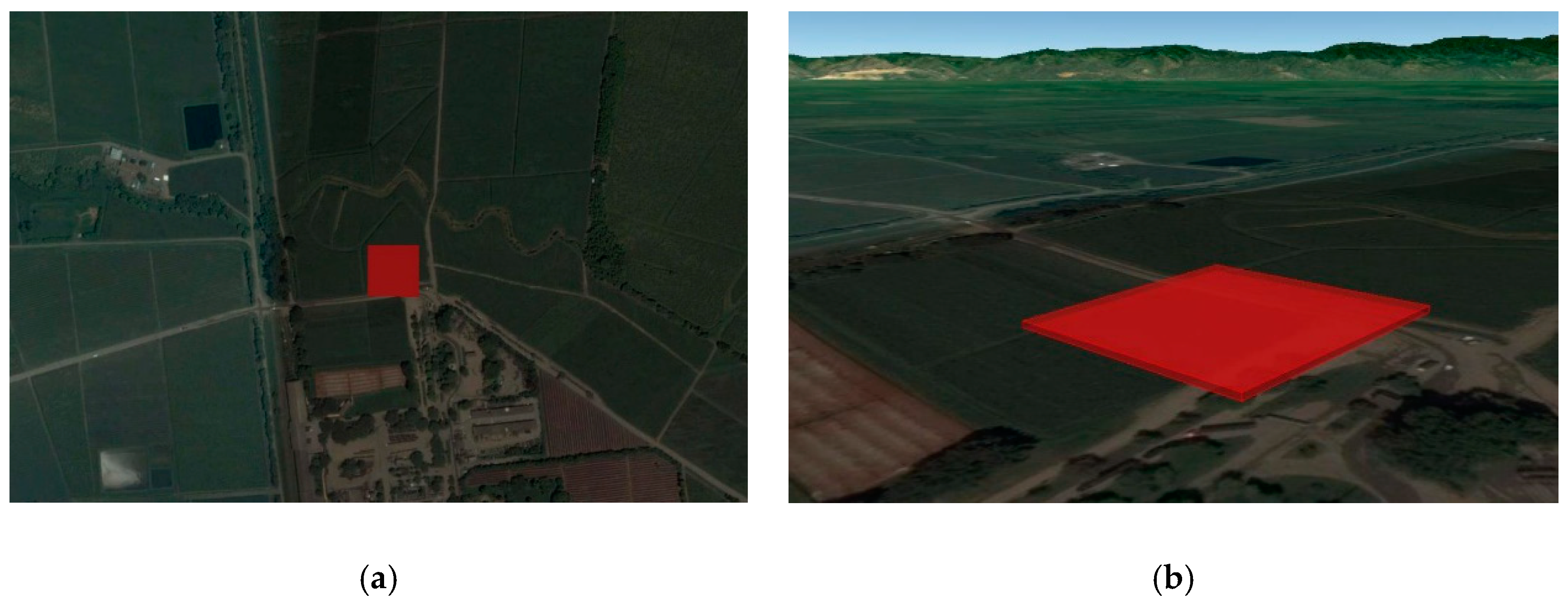
A grid of discrete receptors was defined within the computational domain with a resolution of 100 m over an area of 10 km × 10 km, as shown in Figure 1. Although the results do not depend on the location of the area under consideration, for illustrative purposes, we used the Valle del Cauca region, located in southwest Colombia, which is one of the most important areas of sugarcane cultivation. Colombia is the seventh producer of sugarcane worldwide, and where approximately 16,425 ha are burned per year, and where on average 1.5–2 ha are burned per burning event [19].
2.2. Air Dispersion Model
In this work, we used AERMOD to study the dispersion of the pollutants produced inside the burning area. As stated above, this model is recommended by the USEPA when their results are planned to be used for regulatory purposes. It is a steady-state model that assumes that pollutants concentration downwind the area source follows a Gaussian distribution in the vertical and horizontal direction of the plume, according to Equation (1).
where C is the pollutant concentration (g/m3); Q is the pollutant emission rate (g/s); u is the horizontal wind speed along the plume centerline (m/s); H is the height of emission plume centerline above ground level (m); and are the vertical and horizontal standard deviation of the emission distribution (m), respectively; and f and g are the vertical and horizontal dispersion parameters, respectively.
Gaussian models, and specifically AERMOD, do not allow, on the first instance, to model sources that change their position over time. As an approximation, we assumed that the entire emission source area burns simultaneously, but at a rate such that the emission rate of pollutants (g/s) remains constant. In Section 3, we will show that this assumption is acceptable for this study because the size of the influence area is independent of the size of the burning area being considered.
2.3. Meteorology
High wind speeds contribute to pollutant dispersion but it could also extend the size of the influence area. Low wind speeds generate high concentration of pollutants near the source. The fact that dispersion phenomena is highly dependent of the meteorological conditions hampers the process of generalizing the results obtained. To overcome this difficulty, we studied the dispersion of pollutants generated by agricultural burning under very diverse meteorological conditions. Datasets with 1–5 years of 1-h meteorological conditions from the USA and Colombia were used, since they represent scenarios with extreme weather characteristics during the different seasons of the year. Table 2 presents the list of meteorological data used in this study and Appendix A. shows their respective wind roses. Only meteorological datasets with 100% of data availability were used in work.
2.4. Estimation of the Pollutants’ Mass Emission Rates
The mass emission rate Ei,j (kg/s) of pollutant i emitted by a given crop burning j, was estimated through Equation (2), where Lj (kg/m2) is the amount of biomass that is typically produced by crop j per unit of cultivated area, and Sj (m2/s) is the burning rate [22].
In this equation, E*i,j (kg/kg) is the emission factor and it describes the amount of pollutant i typically emitted per unit mass of crop j. Multiple studies have been conducted to determine the emission factors associated with agricultural burning under controlled conditions [1] and by field measurements [23]. Table 1 shows E*i,j and Lj for several crops. It shows that sugarcane has the largest loading factor. For this crop, Table 3 presents the emission factors reported by different authors, among which, large variations are observed. In this study, we adopted the emission factors reported by the USEPA [22].
The burning rate (Sj in m2/s) depends on multiple factors, including wind speed and crop moisture content. Given the difficulty of finding values reported in the literature for this variable, a constant value was assumed as a first approximation. For the case of sugarcane, we consulted companies in the sugarcane industry, and they reported an approximate value of 1 ha/day. However, it depends on the length and the number of lines used as starting flame fronts.
2.5. Determination of the Influence Area
For a given set of meteorological conditions (temperature, humidity, solar radiation, wind speed and direction), AERMOD estimates the pollutant concentration at every receptor located nearby the burning area. The process is repeated every hour as meteorological data are reported in this format. Given the short-term nature of agricultural burnings, we focused only on human short-term (24 h) exposure. Therefore, we set up AERMOD to calculate at every receptor the 24 h average pollutant concentration and to record only the maximum value obtained after one year of meteorological data (or the number of years of meteorological data availability). Finally, we selected all those receptors where pollutant concentration exceeded its respective threshold value specified in the NAAQS. The combination of all those receptors made up the influence area of agricultural burning.
The largest influence area is produced by the crop with the largest emission rate of the pollutant with the highest hazard to human health. According to Table 1 and Equation (2), for the case of sugarcane, the pollutant with the highest mass emission rate is PM10. Although the PM10 emission factor for sugarcane is one of the lowest among the different crops listed in Table 1, sugarcane is the crop with the highest loading factor.
The hazard of a pollutant can be quantified as the inverse of its threshold value specified in the NAAQS. According to the American Conference of Governmental Industrial Hygienists (ACGIH), the threshold limit values (TLVs) are the maximum average airborne concentration of a hazardous material to which healthy adult workers can be exposed during an 8-h workday and 40-h workweek—over a working lifetime—without experiencing significant adverse health effects. They represent the opinion of the scientific community that exposure at or below the level of the TLV does not create an unreasonable risk of disease or injury [3]. Aiming to provide public health protection, including protecting the health of “sensitive” populations such as asthmatics, children, and the elderly, the environmental authority specifies those threshold limit values in the NAAQS for short time periods of exposure (3, 8, or 24 h depending of the pollutant) and for long time periods of exposure (one year) [14,15,16,17,18,19,20,21,22,23,24]. In this work, we only consider short-term exposition, as agricultural burnings are short-term events. Table 4 lists the USEPA maximum recommended values for short-term exposition.
Aiming to identify the scenario that produces the largest agricultural burning influence area, we defined the risk index (Ii,j) for pollutant i generated from crop j, according to Equation (3). In this equation, AQi is the NAAQS threshold value for pollutant i. The crop and pollutant with maximum value for Ii,j defines the largest area of influence. Table 4 shows the Ii,j* obtained for the case of sugarcane crops (j* = sugarcane). It shows that PM2.5 has the largest Ii,j* and therefore it is the pollutant that defines the influence area for the burning of sugarcane crops.
3. Results
We studied the effect of the meteorology, emissions rate and size of the burning area. For illustrative purposes, we report results for the case of sugarcane burning. However, these results are valid for any crop.
3.1. The Effect of Meteorological Conditions on Pollutant Concentration
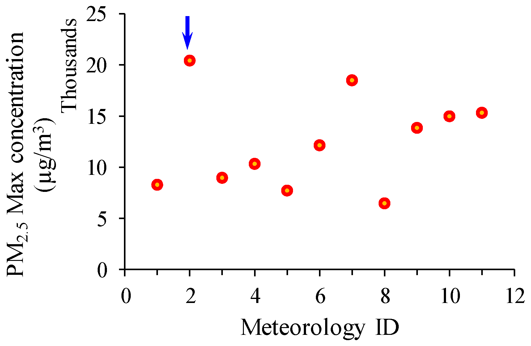
As a first step, we studied the effects of meteorology on the dispersion of pollutants. Arbitrarily, we kept the PM2.5 emission rate constant at 1 g/s over a burning area of 1 ha. As expected, meteorology significantly affects PM2.5 concentration at ground level. Figure 2 presents the daily maximum concentration obtained at any receptor over an extension of 10 km × 10 km, after considering the datasets of 1-h meteorological data listed in Table 2. This figure indicates that the meteorological data No. 2 (Minnesota) induced the highest level of pollutant concentration. This meteorology has an average temperature of 4.5 °C and wind speed of 2.7 m/s with no preferential wind direction. Besides low average wind speed, we could not identify a special characteristic of this meteorology that makes it the worst-case scenario. From now on, we only consider this meteorology as it constitutes the scenario that produces the highest concentrations.
3.2. The Effect of Emission Rate on Pollutant Concentration
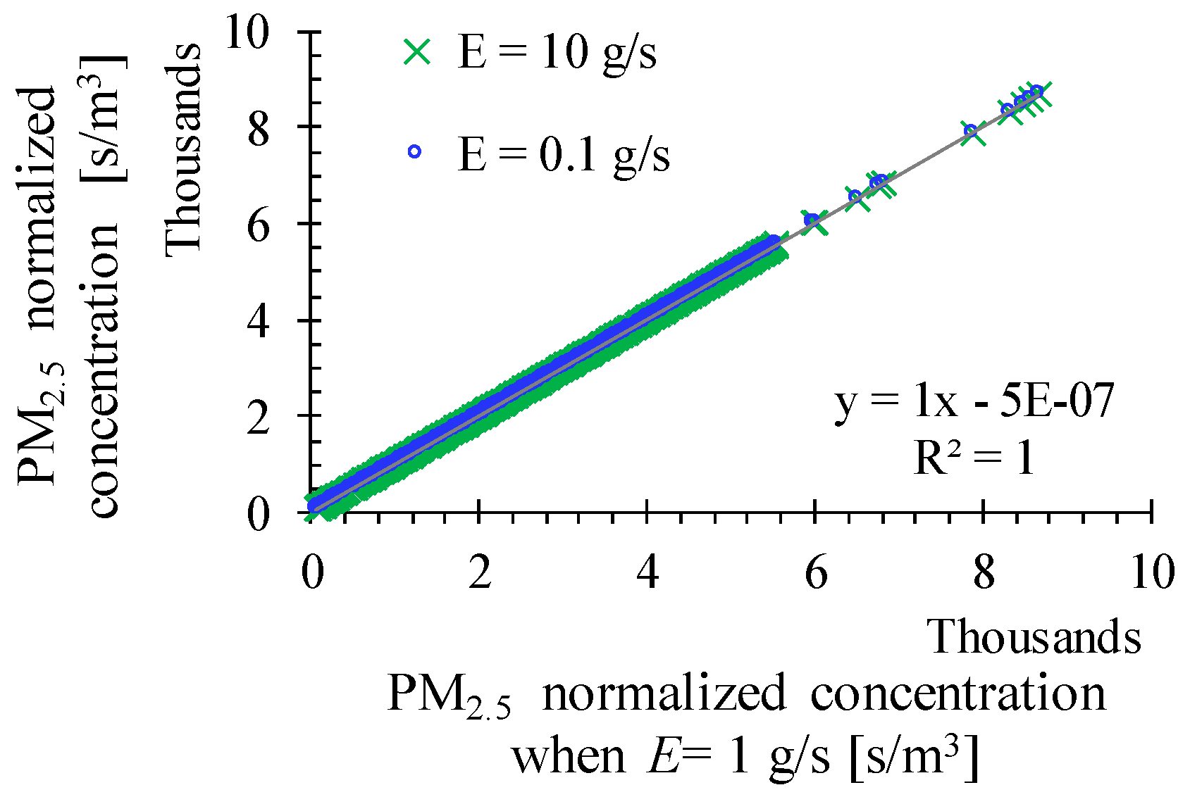
AERMOD has a linear response to changes in emissions. Aiming to confirm this expected behavior, a base emission of 1 g/s was used. This emission was multiplied by 0.1 and 10. We set these values as the new emissions rates and observed PM2.5 concentrations nearby the emission source as predicted by AERMOD. Figure 3 compares PM2.5 concentration obtained at every receptor in the base case scenario against the corresponding concentrations obtained with different emission rates. This comparison was performed in terms of normalized concentration, i.e., concentration divided by the emission rate. Figure 3 shows that all data points fall within the 45-degree line, regardless of the emission rate, confirming that, according to AERMOD, PM2.5 concentration, at ground level, nearby the emission source is proportional to the emission rate.
3.3. Determination of the Influence Area
As explained above, due to the short-term nature of the agricultural burning events, and because those events could happen at any time of the year, the determination of the influence area requires:
- The AERMOD determination of daily maximum concentrations, obtained at each receptor over the computational domain along the simulation time (1–5 years of 1 h meteorological data). The simulation should be carried out for the case of the riskiest pollutant at the emission rate calculated for that pollutant and crop of interest, in this case, PM2.5 and sugarcane, respectively.
- A comparison of the obtained results against the threshold value specified in the NAAQS for short-term exposure to the riskiest pollutant, in this case, 50 µg/m3 for 24 h of human exposure to PM2.5.
Figure 4 shows the maximum daily PM2.5 concentration obtained at each receptor located over a 10 km × 10 km region that surrounds a squared burning area of 1 ha with an hypothetical emission rate of E = 18.6 g/s. It shows that, due to the random wind direction, the influence area does not exhibit any regular shape. Therefore, for the case of agricultural burning, we redefined the influence area as the circle whose radio includes all areas where pollutant concentrations exceed the air quality standards defined by local environmental authorities.
Afterwards, we ran a set of cases changing the size of the area source from 1 m2 to 20 ha and observed their resulting influence areas. As farmers partially control the burning rate by controlling the length and number of lines of starting fire fronts, we considered two alternatives:
- Farmers burn simultaneously the entire area, keeping the number of starting fire fronts per unit area constant. This alternative implies that, regarding of the burning area size, the burning event will be completed within the same period of time of the base case scenario (1 ha). It implies that the burning rate and the emission rate of pollutants per unit area remain constant. However, the total emission rate increases, with respect to the base case scenario, proportionally to the size of the area under consideration.
- Farmers burn sequentially one-unit area after another, increasing the duration of the burning event proportionally to the area size. This alternative implies that the total emission rate remains constant.
In real practice, farmers burn with a combination of both alternatives and therefore we considered this third alternative in our simulations. In all cases, we reported the size of the resulting influence area as the radii of the resulting influence area minus the edge-size of the burning area.
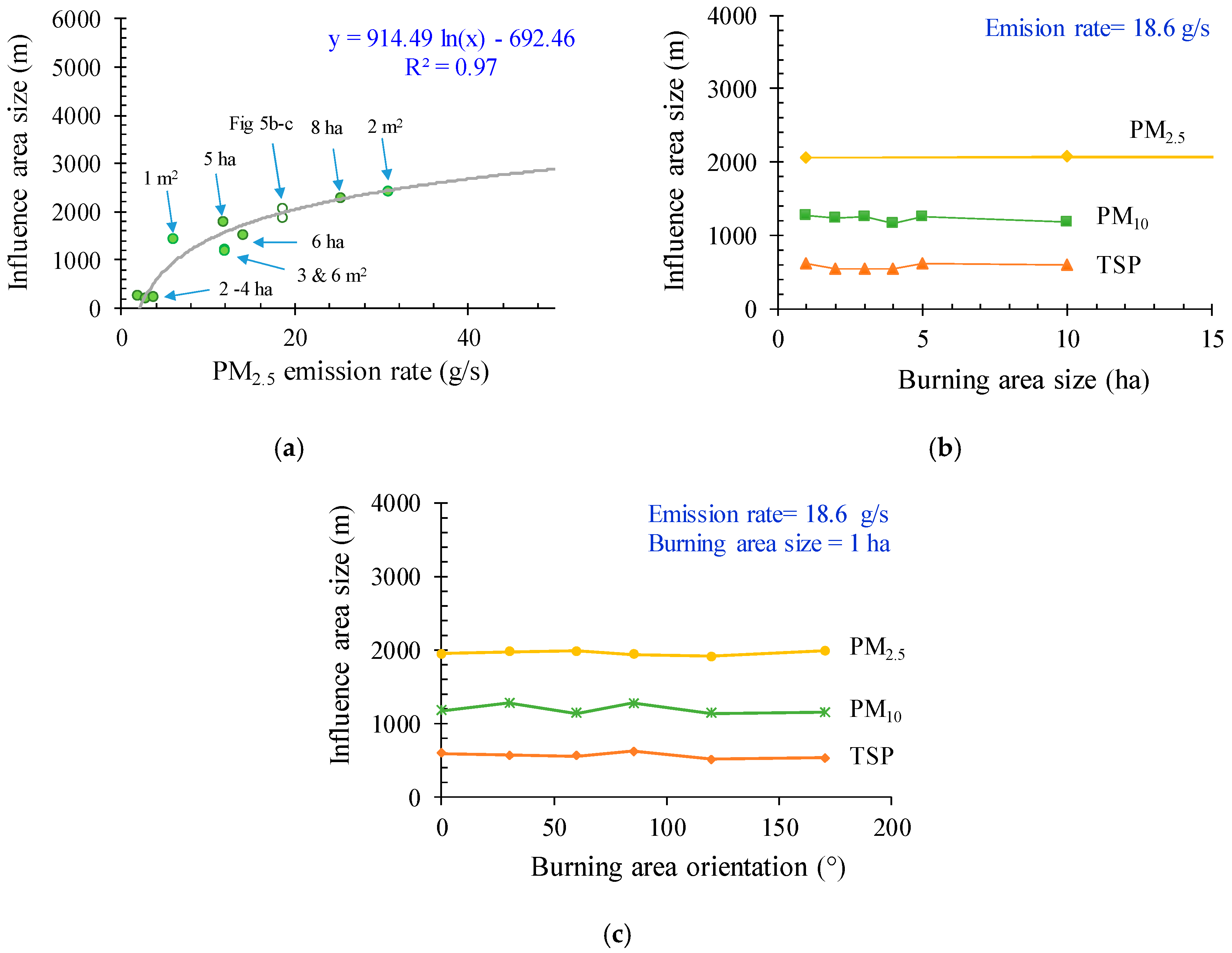
We determined the size of the influence area generated by an area source of 1 ha, varying the emission rate. The obtained results are plotted in Figure 5a. It shows that the size of the influence area increases with the emission rate, following a logarithm profile. This profile crosses the area size axis at an emission rate of about 2 g/s. This means that farmers can burn at a rate smaller than this critical rate generating a negligible influence area. For the case of sugarcane, this value means a maximum burning rate of 1.5 ha/day.
When the emission rate remains constant, the size of the influence area remains constant regardless of the size of the burning area (Figure 5b). The burning of 1 m2 at a given emission rate produces the same size of influence area as the burning of 1 ha at the same emission rate. The difference is that, under these circumstances, it takes 104 times longer to complete the burning task of 1 ha than of 1 m2. This result implies that the size of the influence area is determined by the burnings near the edge of the area source. Aiming to observe the variation of these results with the orientation of the area source, we varied it from 0–170 degrees. The results are presented in Figure 5c. For the case of an area source of 1 ha, with an emission rate of 18.6 g/s, under all orientations that we ran, the influence area was ~2000 m considering PM2.5 as the limiting pollutant. The influence area for PM10 and TSP (Total Suspended Particles) were ~1500 and 500 m, respectively.
Finally, we considered burning areas with shapes different from a square. The area of any irregular polygon can be constructed as the combination of multiple squares of different sizes. Using the principle of superposition, the influence area produced by the area source of irregular shape is the union of the influence areas generated by each independent squared area. Therefore, the influence area generated by the burning of crops cultivated on areas of any shape is the area band that surrounds the burning area. These results are independent of the type of crop or biomass being burned.
3.4. Recommendations for Policy Makers
In the light of this work, we suggest that policy makers interested in controlling the activity of agricultural burning and/or any open atmosphere biomass burning should be aware of:
- Open atmosphere biomass burning produces short- and long-term negative impacts on human health and the environment. Therefore, this practice should be controlled and eliminated as soon as possible. However, this activity is associated with important economic and social aspects that need to be considered. Therefore, environmental authorities, companies and the people that could be affected, should design in collaboration an action plan with a sustainable approach that ends with the elimination of this activity.
- Despite the efforts made by the scientific community to develop tools to assess accurately the impact of open biomass burning, several unresolved aspects and uncertainties remain related to: (i) the amount of biomass burned per crop; (ii) the emission factors for the relevant pollutants per crop; (iii) the understanding and modeling of the pollutant dispersion phenomena; and (iv) secondary effects such as changes in atmospheric dynamics and alterations in the cloud formation processes.
- We used AERMOD to model the dispersion of the pollutants produced during agricultural burning events. This model is recommended by the USEPA for this type of applications. It means that, even though there could exist more accurate models for modeling agricultural burnings, AERMOD is the model that should be used for regulatory purposes, as it is well accepted by the scientific community and environmental authorities.
- Aiming to design public policies to control agricultural burning, the purpose of modeling the dispersion of the pollutants generated by this activity is to assess the environmental impact caused by the agricultural burning of any crop under a worst case but real scenario, considering all the possible pollutants that could be generated. In this regard, it is out of the scope of the present work to reproduce any measurements of pollutant concentration obtained nearby agricultural burning.
Based on the results obtained in this work, we propose that the environmental authorities:
- Limit any agricultural burning or any open atmosphere biomass burning to emissions rates smaller than 2.0 g/s calculated using Equation (2) and data in Table 1, for all pollutants regulated in the NAAQS. According to Figure 5a, this emission rate produces an influence area of negligible size. For the case of sugarcane, this counter-measure limits the burning rate to ~1,5 ha/day, which could be inappropriate for the current operation of the sugarcane industry.
- Determine the distance from the cultivated area to the location of the nearest household and use that distance as the size of an acceptable influence area. Then, use Figure 5a to determine the maximum allowable emission rate, which is directly related to the number of hectares that can be burned per day.
- The implementation of a burning management program that involves previous alternatives. This program divides the cultivated area in subareas, each of them with different distances to the nearest household. For each subarea, Figure 5a limits the maximum burning rate. Then, the burning management program establish the sequence that each area could be burned at the given burning rates. No two areas can be burned simultaneously.
4. Conclusions
Aiming to design public policies to control agricultural burning, we assessed the environmental impact generated by this activity. We used AERMOD to determine the concentration of the pollutants generated by this activity on the areas nearby the burning area (cultivated crop). We considered a wide range of meteorological conditions, burning rates, geometries, and sizes of burning areas.
The area influenced by a given agricultural burning is the largest area where the concentration of any of the pollutant under consideration exceeds its maximum threshold values established in the local atmospheric air quality standards (NAAQS). Results show that this area is a band around the cultivated area whose size increase with the emission rate of the riskiest pollutant (Figure 5a), but it does not depend on size of the burning area. The risk of a pollutant was quantified as the ratio of their emission rate to its threshold value established in the NAAQS.
The emission rate is proportional to the burning rate. As farmers control burning rate by controlling the length and number of starting flame fronts, we proposed the elaboration of a public policy to limit the burning rate in the way that no households are located within the resulting influence area. This proposal should be taken as a transitional stage towards a policy of no agricultural burnings in consideration of their adverse effects on the environment.
Author Contributions
D.F.P. Software, formal analysis, investigation, and original draft preparation. J.I.H. Conceptualization, formal analysis, writing—review and editing, and supervision.
Funding
This research was financed by the Mexican Council for Science and Technology (CONACYT) and by the Colombian Ministry of the Environment.
Acknowledgments
This study was partially financed by the Colombian Ministry of the Environment, the Mexican Council for Science and Technology (Consejo Nacional de Ciencia y Tecnología-CONACYT), and CAIA Engineering.
Conflicts of Interest
The authors declare no conflict of interest.
Appendix A. Wind Roses Obtained for Each Set of Meteorological Data Used in This Study
| Name | Year | Country | Wind Rose Diagram | Name | Year | Country | Wind Rose Diagram |
| San Diego | 2009 | USA |  | Zavala | 2008–2012 | USA |  |
| Minnesota | 2008–2012 | USA |  | Pico | 2008–2012 | USA |  |
| Texas | 1990 |  | Descanso | 2009 | Colombia |  | |
| Michigan | 2008–2012 | USA |  | Cerro largo | 2009 | Colombia |  |
| Alaska | 1990 | USA |  | Rubiales | 2013 | Colombia |  |
| Los Angeles | 2012-2016 | USA |  |
References
- Holder, A.L.; Gullett, B.K.; Urbanski, S.P.; Elleman, R.; O’Neill, S.; Tabor, D.; Mitchell, W.; Baker, K.R. Emissions from prescribed burning of agricultural fields in the Pacific Northwest. Atmos. Environ. 2017, 166, 22–33. [Google Scholar] [CrossRef]
- Ferreira, L.E.N.; Muniz, B.V.; Bittar, T.O.; Berto, L.A.; Figueroba, S.R.; Groppo, F.C.; Pereira, A.C. Effect of particles of ashes produced from sugarcane burning on the respiratory system of rats. Environ. Res. 2014, 135, 304–310. [Google Scholar] [CrossRef] [PubMed]
- ACGIH. Threshold Limit Values (TLVs) and Biological Exposure Indices (BEIs). Appendix B. Signature publications. 2012. Available online: https://www.nsc.org/Portals/0/Documents/facultyportal/Documents/fih-6e-appendix-b.pdf (accessed on 4 April 2019).
- Sahai, S.; Sharma, C.; Singh, S.K.; Gupta, P.K. Assessment of trace gases, carbon and nitrogen emissions from field burning of agricultural residues in India. Nutr. Cycl. Agroecosyst. 2011, 89, 143–157. [Google Scholar] [CrossRef]
- Wieser, U.; Gaegauf, C.K. Nanoparticle emissions of wood combustion processes. In Proceedings of the First World Conference and Exhibition on Biomass for Energy and Industry, Sevilla, Spain, 5–9 June 2000; pp. 805–808. [Google Scholar]
- Jimenez, J.; Wu, C.-F.; Claiborn, C.; Gould, T.; Simpson, C.D.; Larson, T.; Liu, L.-J.S. Agricultural burning smoke in eastern Washington—part I: Atmospheric characterization. Atmos. Environ. 2006, 40, 639–650. [Google Scholar] [CrossRef]
- Badarinath, K.V.S.; Kumar Kharol, S.; Rani Sharma, A. Long-range transport of aerosols from agriculture crop residue burning in Indo-Gangetic Plains-A study using LIDAR, ground measurements and satellite data. J. Atmos. Solar-Terrestrial Phys. 2009, 71, 112–120. [Google Scholar] [CrossRef]
- Akagi, S.K.; Yokelson, R.J.; Wiedinmyer, C.; Alvarado, M.J.; Reid, J.S.; Karl, T.; Crounse, J.D.; Wennberg, P.O. Emission factors for open and domestic biomass burning for use in atmospheric models. Atmos. Chem. Phys. 2011, 11, 4039–4072. [Google Scholar] [CrossRef] [Green Version]
- Chen, J.; Li, C.; Ristovski, Z.; Milic, A.; Gu, Y.; Islam, M.S.; Dumka, U.C. A review of biomass burning: Emissions and impacts on air quality, health and climate in China. Sci. Total Environ. 2017, 579, 1000–1034. [Google Scholar] [CrossRef] [PubMed]
- Arbex, M.A.; Martins, L.C.; de Oliveira, R.C.; Pereira, L.A.A.; Arbex, F.F.; Canҫado, J.E.D.; Saldiva, P.H.N.; Braga, A.L.F. Air pollution from biomass burning and asthma hospital admissions in a sugar cane plantation area in Brazil. J. Epidemiol. Community Health 2007, 61, 395–400. [Google Scholar] [CrossRef] [PubMed] [Green Version]
- Mazzoli-Rocha, F.; Bichara Magalhães, C.; Malm, O.; Hilário Nascimento Saldiva, P.; Araujo Zin, W.; Faffe, D.S. Comparative respiratory toxicity of particles produced by traffic and sugar cane burning. Environ. Res. 2008, 108, 35–41. [Google Scholar] [CrossRef]
- EPA. Solid Waste Disposal 2.5-1 Open Burning. 1995; 92. Available online: https://www3.epa.gov/ttn/chief/ap42/ch02/final/c02s05.pdf (accessed on 4 April 2019).
- Prado, G.F.; Zanetta, D.M.T.; Arbex, M.A.; Braga, A.L.; Pereira, L.A.; de Marchi, M.R.; de Melo Loureiro, A.P.; Marcourakis, T.; Sugauara, L.E.; Gattás, G.J.; et al. Burnt sugarcane harvesting: Particulate matter exposure and the effects on lung function, oxidative stress, and urinary 1-hydroxypyrene. Sci. Total Environ. 2012, 437, 200–208. [Google Scholar] [CrossRef]
- World Health Organization. Evolution of WHO Air Quality Guidelines: Past, Present and Future; WHO Regional Office: København, Denmark, 2017. [Google Scholar]
- Wagner, J.; Naik-Patel, K.; Wall, S.; Harnly, M. Measurement of ambient particulate matter concentrations and particle types near agricultural burns using electron microscopy and passive samplers. Atmos. Environ. 2012, 54, 260–271. [Google Scholar] [CrossRef]
- Mugica-Alvarez, V.; Hernández-Moreno, A.; Valle-Hernández, B.L.; Espejo-Montes, F.; Millán-Vázquez, F.; Torres-Rodríguez, M. Characterization and modeling of atmospheric particles from sugarcane burning in Morelos, Mexico. Hum. Ecol. Risk Assess. Int. J. 2017, 7039, 1–16. [Google Scholar] [CrossRef]
- Hiscox, L.; Flecher, S.; Wang, J.J.; Viator, H.P. A comparative analysis of potential impact area of common sugar cane burning methods. Atmos. Environ. 2015, 106, 154–164. [Google Scholar] [CrossRef]
- Carney, W.; Spicer, B.; Stegall, B.; Borel, C. Louisiana Smoke Management Guidelines for Sugarcane Harvesting. 2000. Available online: https://www.lsuagcenter.com/NR/rdonlyres/8AAEF1B2-EFA6-40A0-AC59-654C15894EE9/12567/smoke_management3.pdf (accessed on 4 April 2019).
- Sornpoon, W.; Bonnet, S.; Kasemsap, P.; Prasertsak, P.; Garivait, S. Estimation of emissions from sugarcane field burning in Thailand using bottom-up country-specific activity data. Atmosphere 2014, 5, 669–685. [Google Scholar] [CrossRef]
- Zhang, H.; Hu, J.; Qi, Y.; Li, C.; Chen, J.; Wang, X.; He, J.W.; Wang, S.X.; Hao, J.M.; Zhang, L.L.; et al. Emission characterization, environmental impact, and control measure of PM2.5 emitted from agricultural crop residue burning in China. J. Clean. Prod. 2017, 149, 629–635. [Google Scholar] [CrossRef]
- Madriñán Palomino, C.E. Compilación y análisis sobre contaminación del aire producida por la quema y la requema de la caña de azúcar, saccharum officinarum L. en el valle geográfico del río cauca. 2002. Available online: http://bdigital.unal.edu.co/cgi/export/5039/ (accessed on 4 April 2019).
- US EPA. AP 42, Fifth Edition, Volume I Chapter 13: Miscellaneous Sources. Section 13.2.1. 2011. Available online: https://www3.epa.gov/ttnchie1/ap42/ch13/ (accessed on 4 April 2019).
- Fang, Z.; Deng, W.; Zhang, Y.; Ding, X.; Tang, M.; Liu, T.; Wang, X. Open burning of rice, corn and wheat straws: Primary emissions, photochemical aging, and secondary organic aerosol formation. Atmos. Chem. Phys. 2017, 17, 14821–14839. [Google Scholar] [CrossRef]
- US EPA. NAAQS Table. Available online: https://www.epa.gov/criteria-air-pollutants/naaqs-table (accessed on 4 April 2019).
- IPCC. 2006 IPCC Guidelines for National Greenhouse Gas Inventory. 2006. Available online: https://www.ipcc-nggip.iges.or.jp/public/2006gl/ (accessed on 4 April 2019).
- Jenkins, B.M.; Turn, S.Q.; Williams, R.B.; Goronea, M.; Abd-el-Fattah, H.; Daniel Jones, A. Atmospheric Pollutant Emission Factors from Open Burning of Agricultural and Forest Biomass by Wind Tunnel Simulations. 1996 California Environmental Protection Agency. Available online: https://www.arb.ca.gov/ei/speciate/r01t20/rf9doc/a932-126_3.pdf (accessed on 4 April 2019).
- França, D.A.; Longo, K.M.; Soares Neto, T.G.; Santos, J.C.; Freitas, S.R.; Rudorff, B.F.T.; Cortez, E.V.; Anselmo, E.; Carvalho, J.A., Jr. Pre-harvest sugarcane burning: Determination of emission factors through laboratory measurements. Atmosphere 2012, 3, 164–180. [Google Scholar] [CrossRef]
- Hall, D.; Wu, C.-Y.; Hsu, Y.-M.; Stormer, J.; Engling, G.; Capeto, K.; Wang, J.; Brown, S.; Li, H.-W.; Yu, K.-M. PAHs, carbonyls, VOCs and PM2.5 emission factors for pre-harvest burning of Florida sugarcane. Atmos. Environ. 2012, 55, 164–172. [Google Scholar] [CrossRef]
- Santiago-De la Rosa, N.; Mugica-Álvarez, V.; Cereceda-Balic, F.; Guerrero, F.; Yá-ez, K.; Lapuerta, M. Emission factors from different burning stages of agriculture wastes in Mexico. Environ. Sci. Pollut. Res. 2017, 24, 24297–24310. [Google Scholar] [CrossRef] [PubMed]
- Mugica-Álvarez, V.; Hernández-Rosas, F.; Magaña-Reyes, M.; Herrera-Murillo, J.; Santiago-De La Rosa, N.; Gutiérrez-Arzaluz, M.; de Jesús Figueroa-Lara, J.; González-Cardoso, G. Sugarcane burning emissions: Characterization and emission factors. Atmos. Environ. 2018, 193, 262–272. [Google Scholar] [CrossRef]
- Colombian Ministry of Environment. Resolution 2254, 1 November 2017. 1 November 2017. Available online: http://www.minambiente.gov.co/images/normativa/app/resoluciones/96-res%202254%20de%202017.pdf (accessed on 4 April 2019).
Figure 1.
(a) Top; and (b) perspective view of the sugarcane area selected in this work to illustrate the estimation of the influence area generated by agricultural burning. The red square represents a burning area of 1 ha.
Figure 1.
(a) Top; and (b) perspective view of the sugarcane area selected in this work to illustrate the estimation of the influence area generated by agricultural burning. The red square represents a burning area of 1 ha.

Figure 2.
Maximum average daily PM2.5 concentrations produced at any receptor over an extension of 10 km × 10 km by the burning of sugarcane biomass on a squared 1 ha area, after considering the datasets of 1-h meteorological data listed in Table 2. The arrow identifies meteorology No. 2 (Minnesota), which produced the highest PM2.5 concentrations.

Figure 3.
Comparison of the normalized PM2.5 concentration at ground level obtained by AERMOD when the emission rate is 0.1 and 10 g/s against the normalized concentration when the emission rate is 1 g/s. Normalized concentration is obtained when the resulting concentration is divided by the emission rate in the source. Results were obtained for a burning area of 1 ha and the Minnesota meteorology dataset.

Figure 4.
PM2.5 ground concentration over a 10 km × 10 km region as result of the sugarcane burning on a square area of 1 ha at a burning rate of 18.6 g/s: (a) 3D representation of PM2.5 concentration; and (b) 2D representation of PM2.5 concentration. The lines in (b) represent circumferences centered in the emission source that limit the obtained influence area when the threshold value is 50 μg/m3 (yellow), 100 μg/m3 (blue) and 300 μg/m3 (red).

Figure 5.
Size of the influence area generated by agricultural burning as function of: (a) emission rate considering different burning area sizes; (b) burning area keeping emission rate constant at 18.6 g/s; and (c) burning area orientation respect to north, keeping constant the emission rate at 18.6 g/s and the burning area at 1 ha.


Table 1.
Emission factors and loading factors for different crops [12].
Table 1.
Emission factors and loading factors for different crops [12].
| Crops | Emission Factors (E*i,j) | Loading Factors (Lj) | |||||
|---|---|---|---|---|---|---|---|
| PM | PM2.5 | CO | NO | Methane | Non-Methane Organic Compounds | ||
| g/Mg | kg/Mg | kg/Mg | kg/Mg | kg/Mg | kg/Mg | Mg/hectare | |
| Unspecified | 11 | 12.5 | 58 | 1.3 | 2.7 | 9 | 4.5 |
| Asparagus | 20 | - | 75 | - | 10 | 33 | 3.4 |
| Barley | 11 | - | 78 | - | 2.2 | 7.5 | 3.8 |
| Corn | 7 | - | 54 | - | 2 | 6 | 9.4 |
| Cotton | 4 | - | 88 | - | 0.7 | 2.5 | 3.8 |
| Grasses | 8 | - | 50 | - | 2.2 | 7.5 | - |
| Pineapple | 4 | - | 56 | - | 1 | 3 | - |
| Rice | 4 | 12.95 | 41 | - | 1.2 | 4 | 6.7 |
| Safflower | 9 | - | 72 | - | 3 | 10 | 2.9 |
| Sorghum | 9 | - | 38 | - | 1 | 3.5 | 6.5 |
| Sugarcane | 2.3–3.5 | - | 30–41 | - | 0.6–2 | 2–6 | 8–46 |
| Alfalfa | 23 | - | 53 | - | 4.2 | 14 | 1.8 |
| Bean (red) | 22 | - | 93 | - | 5.5 | 18 | 5.6 |
| Hay (wild) | 16 | - | 70 | - | 2.5 | 8.5 | 2.2 |
| Oats | 22 | - | 68 | - | 4 | 13 | 3.6 |
| Pea | 16 | - | 74 | - | 4.5 | 15 | 5.6 |
| Wheat | 11 | 4.71 | 64 | - | 2 | 6.5 | 4.3 |
* PM, particulate matter with aerodynamic diameter d < 30 µm; PM2.5, particulate matter with aerodynamic diameter d < 2.5 µm.
Table 2.
Datasets of 1-h meteorological data used to study the dispersion of the pollutants generated during agricultural burnings.
Table 2.
Datasets of 1-h meteorological data used to study the dispersion of the pollutants generated during agricultural burnings.
| ID | Meteorology | Country | Year |
|---|---|---|---|
| 1 | San Diego | USA | 2009–2014 |
| 2 | Minnesota | USA | 2009–2013 |
| 3 | Texas | USA | 1990 |
| 4 | Michigan | USA | 1990 |
| 5 | Alaska | USA | 1990 |
| 6 | Zavala | USA | 2008–2012 |
| 7 | Pico | USA | 2008–2012 |
| 8 | Descanso | Colombia | 2009 |
| 9 | Cerro largo | Colombia | 2009 |
| 10 | Rubiales | Colombia | 2013 |
| 11 | Los Angeles | USA | 2012–2016 |
Table 3.
Sugarcane emission factors reported by several authors expressed as kg of pollutant emitted per Mg of sugarcane biomass burned. Highlighted boxes indicate the values used in this work.
Table 3.
Sugarcane emission factors reported by several authors expressed as kg of pollutant emitted per Mg of sugarcane biomass burned. Highlighted boxes indicate the values used in this work.
| Author, Year | Emission Factor Per Pollutant | ||||||
|---|---|---|---|---|---|---|---|
| BC * | TSP kg/Mg | PM10 kg/Mg | PM2.5 kg/Mg | CO2 g/kg | CO kg/Mg | NO kg/Mg | |
| [22], 2011 | - | - | 2.3−2.5 | - | - | 30−41 | - |
| [25], 2006 | - | - | - | - | 92 | - | - |
| [26], 1996 | - | 4.31−4.64 | 4.51 | 4.19 | - | 55.83 | 3.18 |
| [27], 2012 | - | - | - | 2.6 ± 1.6 | 1303 ± 218 | 65 ± 14 | 1.5 ± 0.4 |
| [28], 2012 | 0.71 ± 0.22 | - | - | 2.49 ± 0.66 | 1255 ± 287 | 9.2 ± 3.3 | - |
| [29], 2017 | 0.158 | - | - | - | 1791.94 ± 145.08 | 68.43 ± 16.23 | 1.63 ± 0.23 |
| [30], 2018 | - | 3.27 ± 0.81 | 1.81 ± 0.14 | 1.19 ± 0.08 | 1618 ± 108 | 25.7 ± 2.04 | - |
* BC, Black carbon; -, no available data; Reference [22] corresponds to the USEPA recommended emission factors.
Table 4.
Colombian NAAQS [31], emission rates for a burning rate of 1 ha/day, and risk indexes calculated for the case of the agricultural burning of sugarcane crops (j = sugarcane).
Table 4.
Colombian NAAQS [31], emission rates for a burning rate of 1 ha/day, and risk indexes calculated for the case of the agricultural burning of sugarcane crops (j = sugarcane).
| Pollutant | Colombian NAAQS | Emission Rate (g/s) | Ii,j (m3/s) | |
|---|---|---|---|---|
| Threshold Values (µg/m3) | Short Term Exposure (h) | |||
| TSP | 300 | 24 | 2.47 | 8.2 |
| PM10 | 100 | 24 | 1.33 | 13.3 |
| PM2.5 | 50 | 24 | 2.23 | 44.6 |
| CO | 5000 | 8 | 21.83 | 0.4 |
| NO2 | 200 | 1 | 2.02 | 10.1 |
© 2019 by the authors. Licensee MDPI, Basel, Switzerland. This article is an open access article distributed under the terms and conditions of the Creative Commons Attribution (CC BY) license (http://creativecommons.org/licenses/by/4.0/).
Share and Cite
MDPI and ACS Style
Prato, D.F.; Huertas, J.I. Determination of the Area Affected by Agricultural Burning. Atmosphere 2019, 10, 312. https://0-doi-org.brum.beds.ac.uk/10.3390/atmos10060312
AMA Style
Prato DF, Huertas JI. Determination of the Area Affected by Agricultural Burning. Atmosphere. 2019; 10(6):312. https://0-doi-org.brum.beds.ac.uk/10.3390/atmos10060312
Chicago/Turabian StylePrato, Daniel F., and Jose I. Huertas. 2019. "Determination of the Area Affected by Agricultural Burning" Atmosphere 10, no. 6: 312. https://0-doi-org.brum.beds.ac.uk/10.3390/atmos10060312
Note that from the first issue of 2016, this journal uses article numbers instead of page numbers. See further details here.