Radar-Based Automatic Identification and Quantification of Weak Echo Regions for Hail Nowcasting


1
School of Electrical and Information Engineering, Tianjin University, Tianjin 300072, China
2
Tianjin Bureau of Meteorology, Tianjin 300074, China
*
Author to whom correspondence should be addressed.
Atmosphere 2019, 10(6), 325; https://0-doi-org.brum.beds.ac.uk/10.3390/atmos10060325
Submission received: 14 May 2019
/
Revised: 12 June 2019
/
Accepted: 12 June 2019
/
Published: 14 June 2019
(This article belongs to the Special Issue Weather Radar Observations of Severe Storms)
Abstract
:The identification of some radar reflectivity signatures plays a vital role in severe thunderstorm nowcasting. A weak echo region is one of the signatures that could indicate updraft, which is a fundamental condition for hail production. However, this signature is underutilized in automatic forecasting systems due to the lack of a reliable detection method and the uncertain relationships between different weak echo regions and hail-producing thunderstorms. In this paper, three algorithms related to weak echo regions are proposed. The first is a quasi-real-time weak echo region morphology identification algorithm using the radar echo bottom height image. The second is an automatic vertical cross-section-making algorithm. It provides a convenient tool for automatically determining the location of a vertical cross-section that exhibits a visible weak echo region to help forecasters assess the vertical structures of thunderstorms with less time consumption. The last is a weak echo region quantification algorithm mainly used for hail nowcasting. It could generate a parameter describing the scale of a weak echo region to distinguish hail and no-hail thunderstorms. Evaluation with real data of the Tianjin radar indicates that the critical success index of the weak echo region identification algorithm is 0.61. Statistics on these data also show that when the weak echo region parameters generated by the quantification algorithm are in a particular range, more than 85% of the convective cells produced hail.
1. Introduction
Severe thunderstorms are the most frequent weather threats to life and property in North China [1,2]. Since thunderstorms have small spatial scales and rapidly evolve, their monitoring and nowcasting commonly rely on weather surveillance radars. Weather radars can capture three-dimensional thunderstorm structure information by volume scanning with a high time and space resolution to determine their severity and development stage.
Upward-moving air in a thunderstorm, which is known as the updraft, is a critical factor in assessing thunderstorm potential [3]. In radar-based severe thunderstorm nowcasting, the identification of updrafts can help forecast some high impact events [4,5,6]. Since the vertical component of radar radial velocity is very small, it is impossible to measure vertical drafts directly. Therefore, the observation of updrafts in single-polarization radars relies on specific morphology signatures of vertical reflectivity, such as the echo overhang, weak echo region, and bounded weak echo region. For dual-polarization radars, differential reflectivity and differential phase are also good indicators of updrafts [7,8,9].
The weak echo region (WER) is a region with low radar reflectivity that is bounded on one side and above by strong echoes [10,11]. It is usually located on the low-altitude inflow side of a thunderstorm. The WER is caused by a strong updraft that carries precipitation particles to the middle levels before they grow to a radar-detectable size [12]. The strong tilted echo above WER is called overhang echo. In Figure 1, the schematic diagram of WER formation is shown. When both sides of a WER are bounded, it is a bounded weak echo region (BWER, also known as an echo-free vault). A BWER is considered to be a sign of a particularly severe thunderstorm.
The formation and growth of hailstones is also closely related to updrafts [14,15,16]. When updrafts carry hydrometeors up above the melting layer, small frozen particles become hail embryos and grow as additional supercooled liquid water freezes onto them. On the condition that updraft strength is sufficient to support large hailstones, and not too strong to eject them out of the growth region, hailstones would reside in the updraft for a long time and become sizeable [10,15,16,17,18,19]. Previous studies also found that broader updrafts in severe thunderstorms are conducive to the growth of hail [19,20,21].
Although updraft-related signatures, such as WERs and BWERs, are helpful to identify hail-producing thunderstorms, they are rarely used in operational forecasting systems due to the lack of a reliable identification algorithm. Most existing identification algorithms aim at BWERs, such as the work of [22,23,24,25]. As part of their storm-labeling system to identify convective updrafts, the authors in [9] proposed a WER identification algorithm. This algorithm searches for WERs by finding if there are at least six of the eight horizontally-adjacent grid volumes with horizontal reflectivity gradients greater than or equal to 8 and column maximum reflectivity greater than or equal to 40 . Obviously, it only considers the interface of the WER and the overhang echo, while ignoring whether there are tilted wall echoes that may lead to false alarms.
Another obstacle to utilize WERs for automatic hail forecasting is uncertainties in the presence of WERs and hailfall. The presence of a WER in a thunderstorm does not necessarily indicate that the updraft has sufficient strength for hail growth [19,26]. In manual forecasting, forecasters can make decisions through comprehensive analysis of WERs based on their experience. In automatic forecasting, categorical values or quantitative values are needed for machine decision making. There are various radar parameters for hail detection. Some of the parameters can be used independently by setting a warning threshold, such as the Waldvogel parameter [27], vertically-integrated liquid water content [28], vertically-integrated liquid water density [29], severe hail index, and probability of severe hail [30].
Some studies proposed various multiparameter approaches. In [31], a simple combine criterion was defined by requiring that at least one of the three parameters exceeds the threshold. In [32], several forecasting variables were combined into one parameter using linear discriminant analysis. In [32,33], logistic regression was used to develop a relationship between radar parameters and hail occurrence. In [34], new combined parameters were defined with the help of principal component analysis. In [35], the performance of mesocyclonic hailstorm detection was improved by combining mesocyclone detection results with radar hail parameters. In [36], hail and no-hail thunderstorms were distinguished by using life-cycle analysis of multiple new radar parameters. In [37,38], semi-supervised clustering and a support vector machine were applied to classify polarimetric radar hydrometeors, respectively. A parameter used in multiparameter models is not necessarily capable of independently distinguishing all samples. However, it may improve overall performance by better distinguishing certain samples.
As a 3D signature, WERs cannot be seen in plan views, but can be exhibited in vertical cross-sections. In retrospective studies and operational hail-suppression programs, vertical cross-sections could help people obtain more information about thunderstorms and make better decisions [39]. However, manually determining the position of a cross-section is time consuming since the information of multiple radar elevations should be considered at the same time.
Based on the above background, we conducted a series of studies around WERs to make better use of them in severe thunderstorm forecasting. The first is the WER detection algorithm, which utilizes their morphological features. It is also the basis of the other algorithms. The second is the automatic vertical cross-section-making algorithm. It can be used as a convenient visualization tool for forecasters in diverse applications. The last is the WER quantification algorithm used for hail detection, which can generate a parameter for each WER. The generated parameter cannot be used to independently detect hail, but it can make better decisions in some cases, so it may improve overall performance in multiparameter models.
The paper is structured as follows: The datasets and study area are specified in Section 2. Section 3 gives a detailed description of the proposed methods, including the WER detection algorithm, the automatic cross-section-making algorithm, and the weak echo region quantification algorithm. The results of validations using real weather radar data and two case examples are provided in Section 4. Finally, Section 5 briefly draws the most important conclusions.
2. Study Area and Data
Our study area was focused on the Beijing-Tianjin-Hebei region in North China. The Beijing-Tianjin-Hebei region is located in the mid-latitude coastal zone, with mountains in the north and west and the Bohai Sea in the east. The terrain is high in the northwest and low in the southeast. This particular terrain leads to frequent thunderstorms [40,41]. Thunderstorm season in this area begins in May and goes until September [42,43]. A general view of the study area is shown in Figure 2a.
Data used in this paper included severe weather event observational data, Doppler weather radar data, and radiosounding data. All radar data were from the single-polarization S-band Tianjin radar. The interval of the radar volume scans was 6 min. Each volume scan included 9 elevations, and the lowest and highest elevation angles were and , respectively. The altitude of the radar was 70.3 m, and its scan range was 230 km. Therefore, at the far end of the radar beam, the minimum detectable height was 2.077 km. All algorithms in this paper were based on the radar plan position indicator (PPI) image, which was generated by bilinear interpolation with a resolution of 1 × 1 km. Radar data were quality controlled, including eliminations of ground clutter [44] and superrefraction [45].
Hail case data were extracted from the severe weather event observational database provided by the China Meteorological Administration. In the database, hail cases are from hail reports of 175 manual observation stations in the study area, which are based on human eye-observations of hailstones of any hail size. The location of the Tianjin radar and the geographical distribution of the manual observation stations are shown in Figure 2b. Data were quality controlled, and only hail records with detailed start and end times were used in this study.
Some analyses needed the heights of the melting layer and the −20 degree layer even though they were not used in the algorithms. Heights were obtained from the products of the Meteorological Information Combine Analysis and Process System (MICAPS) provided by the China Meteorological Administration. The raw files were grid-point field data with a resolution of , which was estimated from radiosounding data. The heights of a specific location were calculated by bilinear interpolation in our system.
In this paper, the algorithms were performed on each convective cell. The convective cell identification algorithm used in this paper was based on Storm Cell Identification and Tracking (SCIT) algorithm [46], but some modifications were made to identify cells in PPI images instead of radial images. SCIT identifies 1D storm segments in radial reflectivity data and then combines individual storm segments into 2D storm components based on spatial proximity. We substituted these two steps by a border-following algorithm proposed by [47]. After binarizing the image with different reflectivity thresholds, the border-following algorithm can directly extract all the 2D connected components, which is similar to the 2D storm components of SCIT. Finally, 3D convective cells were obtained by using the same method as SCIT. Since we mainly focused on severe thunderstorms, in order to relieve computing pressure, the cells with a maximum reflectivity of less than 40 were excluded from the study.
The dataset of convective cells for evaluation was divided into two subsets, one for the detection algorithm and the other for the quantification algorithm. The subset for the detection algorithm contained the cells from May–September 2015, which were manually labeled when there were WERs inside. The method of labeling is described in Section 4.1. The subset for the quantification algorithm involved cells from May–September of 2011–2015. For this subset, we used the following methods to label cells as hail-producing convective cells (positive samples) according to hail case data. First, the cell nearest to the record location within 10 km at the record time from the hail reports was manually labeled. Then, we tracked backward from this cell to find all related convective cells in the same hail case because report time was commonly lagging and there were also WERs in the cumulus stage. There are, however, automatic tracking algorithms such as thunderstorm identification, tracking, analysis, and nowcasting (TITAN) [48], SCIT [46], optical flow [49], and some other advanced methods [50,51]. Errors were unavoidable for automatic algorithms, especially on the condition that there was cell merging and splitting. Therefore, cells were manually tracked to ensure that hail samples were reliable. Finally, 823 cells from 93 hail cases were labeled as hail samples.
Besides the positive set, a negative set that contained no-hail convective cells was prepared for comparison. However, hail cases were easy to miss due to the observation means and the large variability of a hail-swath [52]. Since the probability of hail occurrence was low, the numbers of positive and negative samples were also hugely imbalanced. Consequently, treating all unlabeled cells as negative samples may enormously influence the results. Therefore, after obtaining all identified cells in the dataset, we performed the following filter work to make the negative sample set as clean as possible. On the one hand, all cells that were close to any hail record in time and space were excluded. The specific rule was that when an observation station within 50 km from a cell had a hail record of within one hour, we removed this cell from the negative sample set. On the other hand, if a cell was not located above any observation station, it was filtered out. Most of these samples were located in the Bohai Sea, east of the radar. Through this filtering, although the negative set could not be completely clean, the impact of false-negative samples on the results was reduced.
3. Methodology
In this section, we present detailed descriptions of our methods. The first two subsections are about the WER morphology detection algorithm: Section 3.1 describes the method to find candidate WER areas using their morphological features, and Section 3.2 gives the rules to filter out candidate areas that only look like WERs. In Section 3.3, the automatic vertical cross-section-making algorithm is described. Lastly, Section 3.4 presents the WER quantification method.
3.1. Weak Echo Region Morphology Detection
As the weak echo region is a 3D structure, its identification needs to view multiple elevation scans. However, constructing a 3D image or simultaneously processing multiple images consumes a large amount of computing and storage resources. Considering the real-time detection capabilities, we designed the following method utilizing the 2D echo bottom image of convective cells.
According to the definition, a weak echo region is bounded by at least two strong echo parts, one part above and a tilted wall echo part on one side. The feature of the strong echo part above is that its echo bottom height is high, while echo bottom heights of the tilted wall echo part change rapidly in the same direction. Therefore, the basic idea of our WER identification algorithm was to find a pair of the region with a high echo bottom height and the region with high echo bottom gradients with the same direction. Figure 3 shows the flowchart of the WER detection algorithm. For convenience, we refer to the region with a high echo bottom height as HEBHR and to the region with a high echo bottom gradient region as HEBGR.
To improve the precision of echo bottom images, echo bottom heights were estimated with a linear interpolation method similar to [53]. The echo bottom height of a pixel is calculated as follows:
- Find the minimum elevation where reflectivity exceeds . Call the angle of this elevation and reflectivity value .
- If is the lowest elevation of the radar, set ; otherwise, skip to the next step.
- Obtain the next lower elevation angle and its reflectivity value . Then, echo bottom height is given by:where d is the horizontal distance from this point to the radar location.
Figure 4 shows the schematic diagram of echo bottom estimation.
To use the echo bottom gradient information more conveniently, an echo bottom gradient direction image and an echo bottom gradient magnitude image were generated. The gradient of a non-boundary point is given by:
where is the echo bottom height of the point with coordinates and and are components of the gradient in the direction of the two coordinate axes. The gradient direction of point can be calculated by the formula:
and the magnitude is given by:
After obtaining the needed images, the first step was to find the HEBGRs in which the echo bottom gradient magnitude of each point was large and the gradient direction was similar. They were the possible positions of tilted wall echoes. The way to find HEBGRs is as follows.
- Select a gradient magnitude threshold . Threshold the gradient magnitude image using , that is a pixel in the image was set to zero if its value was less than . Obtain the other connected components using the edge-following algorithm proposed by [47].
- Select an area threshold . Filter out connected components whose area is less than .
- Estimate the standard deviation of the gradient directions in each connected component. As a circular quantity, the standard deviation of gradient directions is given by [54]:is given by the expression:where n is the number of samples.
- Select a gradient direction radian standard deviation threshold . Filter out connected components whose standard deviation is greater than .
Then, for each HEBGR, determine whether there are paired HEBHRs. This can be done by the following steps:
- In the HEBGR, find the point with maximum echo bottom height and the point with minimum echo bottom height . Calculate the height threshold by:where the constant 0.5 is used to make sure that the heights of HEBHR are more than half of the heights of the paired HEBGR.
- Threshold the echo bottom image by . Obtain the other connected components.
- Select area threshold , and filter connected components whose area is less than .
- If an HEBHR has overlapping parts with HEBGR and is not totally included in it, pair them as one candidate location of a weak echo region. Note that an HEBGR may be paired with multiple HEBHRs.
The schematic diagrams of the algorithm are shown in Figure 5.
The thresholds used in the detection algorithm included the minimum echo bottom gradient of HEBGR , the minimum area of HEBGR , the minimum area of HEBHR , and maximum gradient standard deviation . and were used to eliminate noise. We set their values to 10 since a typical WER is larger than that. To acquire the appropriate values of and , we conducted preliminary research by making statistics on several real samples. According to the results, we set to 1 and to 1.2 (the units of both the horizontal and vertical distance are km).
3.2. Result Filter
The detection algorithm presented in the previous subsection identifies WERs by their morphological definition. However, in practice, there are many WER lookalikes that are not caused by updrafts. On the one hand, signatures such as overspreading anvil and three-body scatter spike [55] are morphologically similar to WER. On the other hand, some causes such as fast-moving storms [23] and echo-connecting may make echoes look like WERs. These echoes should be filtered out as much as possible. Therefore, we designed two filters to screen candidate WER locations. Some examples of WER lookalikes are shown in Figure 6.
As WERs are located within thunderstorms, the reflectivity of bounded echoes is strong. In contrast, reflectivity in an anvil or three-body scatter spike is relatively weak. Hence, identification results with only weak reflectivity should be filtered out. Considering the variety of thunderstorms, we used six reflectivity thresholds to run the detection algorithm and kept a result if at least three of them in the same position were identified. The reflectivity thresholds used in this paper were 20, 25, 30, 35, 40, and 45 .
When updrafts flow into convective cells, reflectivity gradients are higher on the low-level inflow side. Therefore, one kind of solution is to recognize tight gradient regions of cells in low-elevation PPI images and discard detection results far away from these locations. However, in our preliminary attempt, we found that the actual situations were too complicated to identify high reflectivity gradient regions and determine whether a high gradient region was the inflow side. In order to improve stability and applicability, we designed a filter method by comparing the gradients of eight different cell directions. The method is presented as follows:
- Build the composite reflectivity image of the lowest three elevations. Calculate the reflectivity gradient of every grid point on this image. The gradient equation is similar to Equation (2), but echo bottom heights are replaced with reflectivity values in units of .
- For each cell, find the centroid of the second maximum reflectivity region. Centering on this point, divide the cell image into eight equal angles, as shown in Figure 7a.
- Calculate the average gradient magnitude of each part. To eliminate noise points, the points whose gradient directions do not point near the center are excluded from calculating.
- Find the part with the maximum average gradient magnitude, and mark it and its two adjacent parts as the possible inflow region. Filter out detection results that have no overlapping area with the possible inflow region, as shown in Figure 7b.
3.3. Automatic Vertical Cross-Section Making
The radar reflectivity vertical cross-section is an important visualization tool to observe the internal structure of thunderstorms. In some applications, such as hail-suppression operations, rapidly and accurately generating vertical cross-sections can help people make decisions [56]. Vertical cross-sections are also able to exhibit the structures of WERs and BWERs. However, manually determining the location of such vertical cross-sections is time consuming and fallible because it needs to observe and analyze multiple elevations at the same time. Consequently, based on the automatic WER detection algorithm, we designed an algorithm to determine the location of a vertical cross-section automatically that can show a clear WER structure.
After a WER is detected, its vertical cross-section line could be determined by a point and a direction as follows. On the one hand, in order to display both the tilted wall echo part and the overhang echo part, the line should pass through the two regions at the same time, that is the line should pass through a certain point in the overlapping area of HEBGR and HEBHR. Thus, we chose the centroid of the maximum reflectivity region in the overlapping area of HEBGR and HEBHR as the point through which the line should pass. Using the centroid of the maximum reflectivity region is to show the most severe part of the thunderstorm. On the other hand, in order to show a clear WER structure, the direction of the straight line is preferably in the direction of the echo tilt. Therefore, we used the average direction of HEBGR given by Equation (6) as the direction of the vertical cross-section line. Examples of vertical cross-sections obtained automatically by this method are shown in Section 4.3.
3.4. Weak Echo Region Quantification
The presence of a WER or BWER means there are updrafts inside thunderstorms, and a strong updraft is a prerequisite for hail formation. Unlike BWERs that commonly indicate particularly severe thunderstorms, the presence of WERs does not always mean the updraft strength is sufficient for hail growth. It would be helpful for hail nowcasting if we could find which WERs are related to hail-producing thunderstorms. Based on this motivation, we attempted to design a WER quantification method that could generate a parameter that reflects a correlation between WERs and hail-producing thunderstorms.
Considering the diversity and complexity of a WER structure, it is difficult to measure directly and represent it with one quantity. An alternative solution is to construct a quantity that is a combination of multiple components. Each component is a simple measurable value of one part of the WER. Several points were considered while selecting the components. First, previous studies found that broader updrafts are favored for enhanced hail growth [17,19,20]. The volume of the WER could reflect updraft width. Second, the echo overhanging the WER contains supercooled liquid water on which hail growth is dependent [26]. Thus, the intensity and volume of overhang echo may be relevant. Third, multiple reflectivity thresholds can be used to adapt to different thunderstorm events. Therefore, the following two kinds of volumes with different reflectivity thresholds were used as the components:
- Volume between the undersurface of the overhang echo and plane of height , denoted by .
- Volume of the overhang echo whose undersurface is higher than , denoted by .
The formulas for estimating and are:
and:
where is the horizontal grid-point set of the area where the WER is located, which is obtained by the detection algorithm, is the grid point of , and are the echo top height and echo bottom height at point , respectively, and is a user-defined height threshold, discussed later. The schematic diagram describing the two parts of volumes is shown in Figure 8.
The setting of height threshold is to eliminate the influence of different minimum detectable heights on volume estimation. As shown in Figure 9a, if the same thunderstorm is detected in different radar ranges, the volumes between the undersurface of the overhang echo and the plane where the lowest radar beams are located are unequal. Therefore, we can make volumes stay constant by specifying the minimum height, as shown in Figure 9b. should be carefully selected according to radar information. When using multiple radars, thresholds should be consistent to ensure that volumes estimated by each radar are of the same standard. If radar altitudes vary, a solution is to limit the effective detection range of some radars. In this paper, , since the lowest detectable height of the far end of the radar beams is 2.077 km.
After obtaining the components, a combination method should be used to construct the quantity. Since the quantity is mainly used to distinguish hail from non-hail, a supervised dimensionality reduction method, such as linear discriminant analysis (LDA), is an ideal choice [57]. LDA is a data-driven method that finds a linear combination of features that characterizes or separates two or more classes of objects. It uses features and class labels to find a projection hyperplane that minimizes interclass variance and maximizes the distance between the projected means of the classes. Compared with unsupervised dimensionality reduction methods, such as principal component analysis, LDA can use class information to obtain a projection with more interclass discrimination. In this task, we applied linear discriminant analysis to a historical dataset that included both hail and non-hail samples and then used the obtained coefficients for a linear combination to construct the quantity (hereinafter referred to as the WER parameter). The equation for WER parameter is:
where N is the number of reflectivity thresholds, is the reflectivity threshold value, and are the volumes estimated using reflectivity threshold , and are coefficients obtained by linear discriminant analysis. The unit of is .
4. Results and Discussion
4.1. Detection Evaluation
We used manually-identified samples to evaluate the performance of the WER detection algorithm. As WERs are easy to miss and some samples are ambiguous, three experienced forecasters from the Tianjin Meteorological Observatory participated in this work. After independent identifications, results were cross-checked, and only samples identified at least twice were confirmed. The data for evaluation were Tianjin radar base data from May–September 2015, which included 32,747 valid volume scans and 16,170 identified severe convective cells. Finally, 294 WER samples were identified.
The contingency table shown in Table 1 contains the evaluation results. Detection errors caused by radar data quality were not counted; where, in the contingency table, a is the number of events that were correctly detected, b is the number of events that failed to be detected, c is the number of false detected nonevents, often referred to as false alarms, and d is the number of undetected nonevents. The probability of detection (POD) and false alarm rate (FAR) are, respectively, given by:
and the critical success index (CSI) [58] is:
From Table 1, it can be seen that both misdetection and false detection were inevitable since the method only used the reflectivity morphological features. By analyzing misses, we found that almost all of them were filtered by the low-elevation reflectivity gradient because the gradient was not obvious at the beginning of the inflow. However, with no filtering procedure, there were more false detections.
Then, we performed the automatic cross-section-making algorithm on all detected samples and manually checked the cross-sections generated by the algorithm. Results showed that all generated cross-sections can exhibited clear WER structures. Examples of cross-sections generated automatically by the algorithm are shown in Figures 14 and 16.
Our experiment system was written in Python with the OpenCV package [59]. The maximum running time of the WER identification and the cross-section making of each cell was 30 ms on a computer with an Intel i7-8700k processor. Therefore, these methods can meet the real-time requirements in most applications.
One thing to note is that the minimum detectable height had a significant impact on the identification of WERs. In this evaluation, we did not limit the range of detections because the true value was manually identified, and WERs occurring below the lowest radar beams are also invisible to people. However, in operational forecasting, effective detection range should be carefully considered according to the altitude and lowest elevation angle of the radar. Otherwise, the algorithm may miss some WERs that could provide valuable information for forecasting. When using multiple radars for detection, a better choice is to set the optimal detection range of each radar.
4.2. Quantification Evaluation
To evaluate the WER quantification method for hail nowcasting, we compared the WER parameters of WERs within hail-producing convective cells with ones in other cells. The dataset used in this evaluation is described in Section 2.
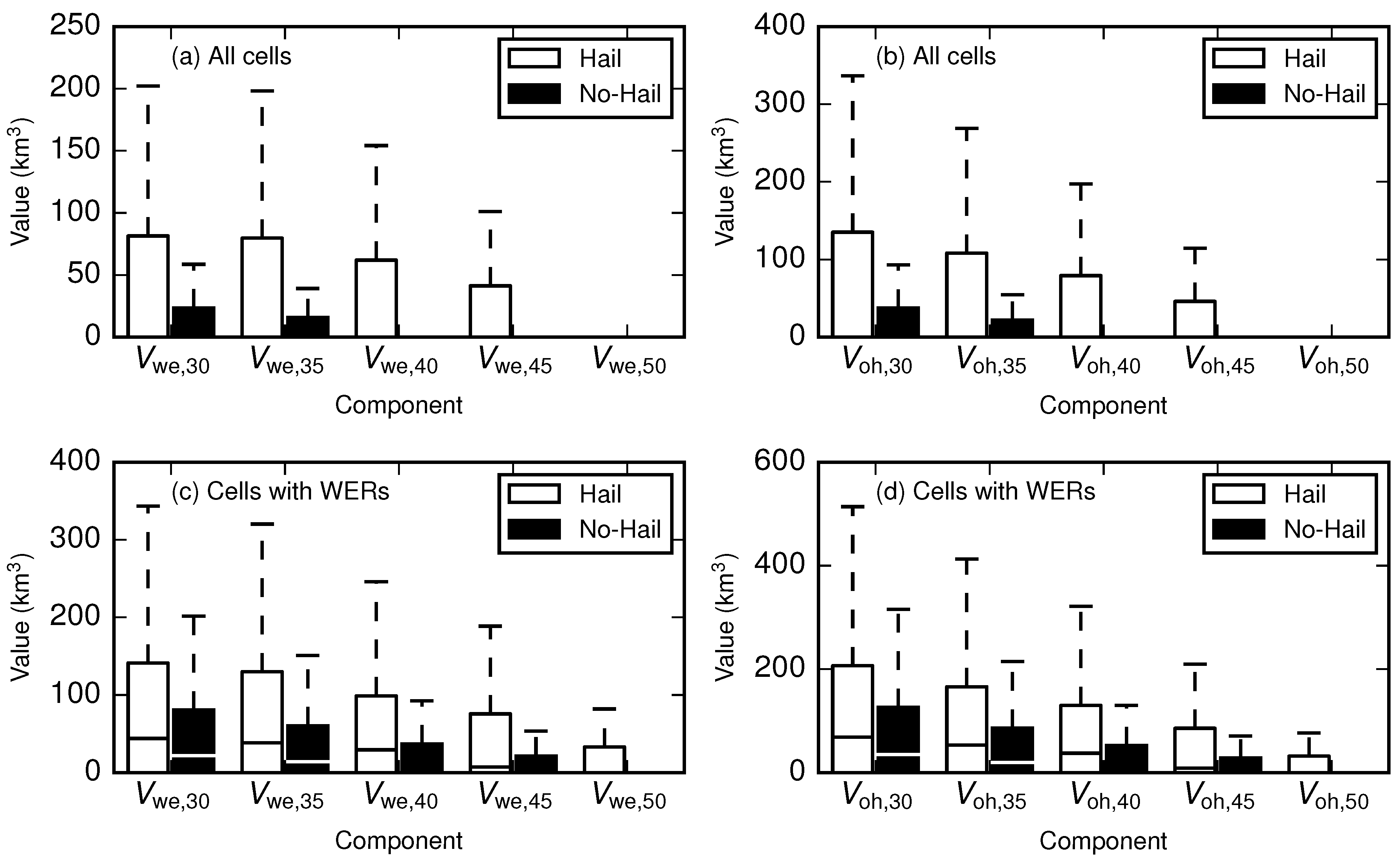
We ran the WER detection algorithm to obtain all cells with WERs and computed the values of and with reflectivity thresholds of 30, 35, 40, 45, and 50 on these cells. The values of the cells without WERs were all set to zero. Figure 10 shows the box plot of the results. From this figure, it can be seen that the median of all components was zero since most cells do not possess WERs. Except for the 50 , the distributions of and with other reflectivity thresholds were significantly different between hail and no-hail convective cells. Rare no-hail cells also have WERs with larger reflectivity than 40 . Therefore, we used and with reflectivity thresholds of 30, 35, 40, and 45 as the components of linear discriminant analysis.
Normalized coefficients determined by linear discriminant analysis are shown in Figure 11. It can be seen that and had the first two large coefficients. Generally, a component with a larger absolute coefficient value is a better predictor in linear discriminant analysis. It is worth noting that had a negative coefficient. As its absolute value was small, this does not mean that was negatively related to hail, but their correlation was not significant and the number of no-hail samples larger.
Figure 12a shows the probability density function of the WER parameters of cells with WERs, which is estimated by Gaussian kernel density estimation with automatic bandwidth selection [60,61]. For no-hail samples, most of their WER parameters were around zero, and very few samples exceeded 150. For hail samples, although most of their values were also near zero, and there were many samples with a WER parameter larger than 150. To compare the proportion of samples with different WER parameters, percentage changes are shown in Figure 12b. From this figure, it can be seen that, when the WER parameter was less than 150, no-hail samples accounted for the majority, while, when the value was in the range of 200–450, hail samples were in the majority. Detailed statistics for samples with values between 200 and 450 found that more than 85% were hail samples.
According to the above results, it is clear that the WER parameter cannot be used to forecast hail-producing thunderstorms alone. However, when values are in a certain range, more than 85% of the samples produced hail. Therefore, it can give a more confident forecast in some cases, and could be used as a parameter in multiparameter models to improve the overall performance of hail nowcasting.
4.3. Case Examples
Two hail cases from the Tianjin radar were used as examples to show the performance of the WER detection algorithm and the automatic vertical cross-section-making algorithm. Figure 13 shows the motion trajectories of cell centroids. Figure 14 shows the composite reflectivity images and the vertical cross-section images of the cells at each time step of Case 1. The line chart in Figure 15 displays the change of over time steps of Case 1. The images and line chart of Case 2 are shown in Figure 16 and Figure 17, respectively. Since the duration of Case 2 was long, only part of the time steps is shown. The vertical cross-sections of reflectivity in these figures were obtained automatically by the proposed algorithm.
For Case 1, the thunderstorm initiated in the south of Beijing and moved toward the south after 14:24 local time (LT = UTC + 8), 10 June 2014. Observation stations on the moving path started to report hail from 15:42 LT. At 14:54 LT, the algorithm started to detect WERs in the south of the cell. As convective cells evolved, WERs became larger. From Figure 15, it can be seen that the WER became largest at 07:54 LT and then began to decay. The cross-section images from 14:54–16:12 LT in Figure 14 show that WERs were bounded on both sides (BWERs).
For Case 2, the strong convective cell formed in the west of Tianjin at 14:30 LT, 27 July 2015. Then, it moved toward the northeast. The earliest hail record was at 16:48 LT. In the life cycle of this case, there were two significant WER processes. First, at 15:18 LT, the algorithm identified a WER in the northeast of the cell, but it lasted for a short time and did not grow large. A more significant WER was detected from 16:30 LT, and it became largest at about 17:00 LT. Figure 16 clearly shows the development of the two WER processes.
5. Conclusions
This paper proposed three algorithms related to weak echo regions, including a WER morphology detection algorithm, an automatic vertical cross-section-making algorithm, and a weak echo region quantification method.
The WER morphology identification algorithm finds candidate WER regions by pairing regions with a high echo bottom height and regions with a high echo bottom gradient, then filters candidate regions that are not caused by updrafts by using low-level reflectivity gradients. Validation results on real data of the Tianjin radar indicate that the identification algorithm had a CSI score of 0.61. Based on the identification algorithm, the automatic vertical cross-section-making algorithm determines the cross-section line by finding a point in the overlapping area of a high echo bottom height region and a high echo bottom gradient region, calculating the average tilt direction of the wall echoes. Two case examples showed that each vertical cross-section generated by the algorithm could exhibit obvious WERs. These two algorithms provide convenient tools for severe thunderstorm analysis that can be used in many applications, such as retrospective studies and operational hail suppression. Compared with manual cross-section making, it can save much time and be more accurate.
The WER quantification algorithm quantifies a WER with the linear combination of several components. The components are volumes of different WER parts, and the coefficients are generated by linear discriminant analysis trained on historical data. Results on Tianjin data showed that, when the WER parameter was between 200 and 450, more than 85% of the samples produced hail. It can be used as an auxiliary parameter in multiparameter forecasting approaches such as logistic regression [33] to improve the performance of hail nowcasting.
Although we used several reflectivity features to filter out WER lookalikes that were not caused by updrafts, detection performance was still limited because the single-polarization radar cannot provide more information. Therefore, applying the algorithm on dual-polarization radars and introducing more parameters may improve performance. As dual-polarization radars are not widely used in some regions, our algorithm is still useful.
In this paper, we only analyzed the relationships between WER parameters and hail-producing thunderstorms. In a future study, we plan to use the WER parameter as a feature in a machine learning classifier [62,63,64] with other classic hail parameters to test how much it can improve overall performance.
Author Contributions
Methodology, J.S.; software, J.S.; validation, D.W.; investigation, D.W.; resources, H.J.; data curation, H.J.; writing, original-draft preparation, J.S.; writing, review and editing, P.W.; supervision, P.W.; project administration, J.S.; funding acquisition, P.W.
Funding
This study was partially supported by the Natural Science Foundation of Tianjin, China, under Grant No. 14JCYBJC21800.
Acknowledgments
The authors would like to thank the Tianjin Meteorological Observatory for providing radar data and weather-station data. We thank the reviewers for their professional suggestions and comments.
Conflicts of Interest
The authors declare no conflict of interest.
Abbreviations
The following abbreviations are used in this manuscript:
| WER | Weak echo region |
| BWER | Bounded weak echo region |
| PPI | Plan-position indicator |
| MICAPS | Meteorological Information Combine Analysis and Process System |
| SCIT | Storm cell identification and tracking |
| TITAN | Thunderstorm identification, tracking, analysis, and nowcasting |
| HEBGR | High echo bottom gradient region |
| HEBHR | High echo bottom height region |
| LDA | Linear discriminant analysis |
| POD | Probability of detection |
| FAR | False alarm rate |
| CSI | Critical success index |
| LT | Local time |
References
- Xiaobo, L.J.Q. Spatial and Temporal Characteristics of Thunderstorm in China. Meteorol. Mon. 2008, 11, 22–30. [Google Scholar]
- Liu, D.; Qie, X.; Peng, L.; Li, W. Charge structure of a summer thunderstorm in North China: Simulation using a regional atmospheric model system. Adv. Atmos. Sci. 2014, 31, 1022–1034. [Google Scholar] [CrossRef]
- Allaby, M.; Park, C. A Dictionary of Environment and Conservation; OUP: Oxford, UK, 2013. [Google Scholar]
- Zhao, Z.; Qie, X.; Zhang, T.; Zhang, T.; Zhang, H.; Wang, Y.; She, Y.; Sun, B.; Wang, H. Electric field soundings and the charge structure within an isolated thunderstorm. Chin. Sci. Bull. 2010, 55, 872–876. [Google Scholar] [CrossRef]
- Cintineo, R.M.; Stensrud, D.J. On the predictability of supercell thunderstorm evolution. J. Atmos. Sci. 2013, 70, 1993–2011. [Google Scholar] [CrossRef]
- Williams, E.R. Meteorological aspects of thunderstorms. In Handbook of Atmospheric Electrodynamics, Volume I; CRC Press: Boca Raton, FL, USA, 2017; pp. 27–60. [Google Scholar]
- Loney, M.L.; Zrnić, D.S.; Straka, J.M.; Ryzhkov, A.V. Enhanced polarimetric radar signatures above the melting level in a supercell storm. J. Appl. Meteorol. 2002, 41, 1179–1194. [Google Scholar] [CrossRef]
- Van Lier-Walqui, M.; Fridlind, A.M.; Ackerman, A.S.; Collis, S.; Helmus, J.; MacGorman, D.R.; North, K.; Kollias, P.; Posselt, D.J. On Polarimetric Radar Signatures of Deep Convection for Model Evaluation: Columns of Specific Differential Phase Observed during MC3E. Mon. Weather Rev. 2016, 144, 737–758. [Google Scholar] [CrossRef] [PubMed]
- Starzec, M.; Homeyer, C.R.; Mullendore, G.L. Storm Labeling in Three Dimensions (SL3D): A Volumetric Radar Echo and Dual-Polarization Updraft Classification Algorithm. Mon. Weather Rev. 2017, 145, 1127–1145. [Google Scholar] [CrossRef]
- Browning, K. Some inferences about the updraft within a severe local storm. J. Atmos. Sci. 1965, 22, 669–677. [Google Scholar] [CrossRef]
- Marwitz, J.D. The structure and motion of severe hailstorms. Part I: Supercell storms. J. Appl. Meteorol. 1972, 11, 166–179. [Google Scholar] [CrossRef]
- Browning, K. The structure and mechanisms of hailstorms. In Hail: A Review of Hail Science and Hail Suppression; Springer: Boca Raton, FL, USA, 1977; pp. 1–47. [Google Scholar]
- Lemon, L. Severe Thunderstorm Evolution-Its Use in a New Technique for Radar Warnings. In Bulletin of the American Meteorological Society; American Meteorological Society: Boston, MA, USA, 1977; Volume 58, p. 676. [Google Scholar]
- Conway, J.W.; Zrnić, D.S. A Study of Embryo Production and Hail Growth Using Dual-Doppler and Multiparameter Radars. Mon. Weather Rev. 1993, 121, 2511–2528. [Google Scholar] [CrossRef] [Green Version]
- Kennedy, P.C.; Detwiler, A.G. A Case Study of the Origin of Hail in a Multicell Thunderstorm Using In Situ Aircraft and Polarimetric Radar Data. J. Appl. Meteorol. 2003, 42, 1679–1690. [Google Scholar] [CrossRef] [Green Version]
- Grant, L.D.; Van Den Heever, S.C. Microphysical and dynamical characteristics of low-precipitation and classic supercells. J. Atmos. Sci. 2014, 71, 2604–2624. [Google Scholar] [CrossRef]
- Nelson, S.P. The influence of storm flow structure on hail growth. J. Atmos. Sci. 1983, 40, 1965–1983. [Google Scholar] [CrossRef]
- Heymsfield, A.J. Case Study of a Halistorm in Colorado. Part IV: Graupel and Hail Growth Mechanisms Deduced through Particle Trajectory Calculations. J. Atmos. Sci. 1983, 40, 1482–1509. [Google Scholar] [CrossRef] [Green Version]
- Dennis, E.J.; Kumjian, M.R. The impact of vertical wind shear on hail growth in simulated supercells. J. Atmos. Sci. 2017, 74, 641–663. [Google Scholar] [CrossRef]
- Foote, G.B. A study of hail growth utilizing observed storm conditions. J. Clim. Appl. Meteorol. 1984, 23, 84–101. [Google Scholar] [CrossRef]
- Miller, L.J.; Tuttle, J.D.; Foote, G.B. Precipitation production in a large Montana hailstorm: Airflow and particle growth trajectories. J. Atmos. Sci. 1990, 47, 1619–1646. [Google Scholar] [CrossRef]
- Smalley, D.J.; Donaldson, R.J. Quantification of severe storm structures. In Proceedings of the 27th Conference on Radar Meteorology, Vail, CO, USA, 9–13 October 1995; American Meteorological Society: Boston, MA, USA, 1995; pp. 617–619. [Google Scholar]
- Lakshmanan, V.; Witt, A. Detection of bounded weak echo regions in meteorological radar images. In Proceedings of the 13th International Conference on Pattern Recognition, Vienna, Austria, 25–29 August 1996; IEEE: Washington, DC, USA, 1996; Volume 3, pp. 895–899. [Google Scholar]
- Lakshmanan, V. Using a genetic algorithm to tune a bounded weak echo region detection algorithm. J. Appl. Meteorol. 2000, 39, 222–230. [Google Scholar] [CrossRef]
- Pal, N.R.; Mandal, A.K.; Pal, S.; Das, J.; Lakshmanan, V. Fuzzy Rule–Based Approach for Detection of Bounded Weak-Echo Regions in Radar Images. J. Appl. Meteorol. Climatol. 2006, 45, 1304–1312. [Google Scholar] [CrossRef]
- Doswell, C. Severe Convective Storms; Springer: Boca Raton, FL, USA, 2001; Chapter 6; Volume 28, pp. 230–231. [Google Scholar]
- Waldvogel, A.; Federer, B.; Grimm, P. Criteria for the detection of hail cells. J. Appl. Meteorol. 1979, 18, 1521–1525. [Google Scholar] [CrossRef]
- Greene, D.R.; Clark, R.A. Vertically integrated liquid water—A new analysis tool. Mon. Weather Rev. 1972, 100, 548–552. [Google Scholar] [CrossRef]
- Amburn, S.A.; Wolf, P.L. VIL density as a hail indicator. Weather Forecast. 1997, 12, 473–478. [Google Scholar] [CrossRef]
- Witt, A.; Eilts, M.D.; Stumpf, G.J.; Johnson, J.; Mitchell, E.D.W.; Thomas, K.W. An enhanced hail detection algorithm for the WSR-88D. Weather Forecast. 1998, 13, 286–303. [Google Scholar] [CrossRef]
- Skripniková, K.; Řezáčová, D. Radar-based hail detection. Atmos. Res. 2014, 144, 175–185. [Google Scholar] [CrossRef]
- López, L.; Sánchez, J. Discriminant methods for radar detection of hail. Atmos. Res. 2009, 93, 358–368. [Google Scholar] [CrossRef]
- Stefan, S.; Barbu, N. Radar-derived parameters in hail-producing storms and the estimation of hail occurrence in Romania using a logistic regression approach. Meteorol. Appl. 2018, 25, 614–621. [Google Scholar] [CrossRef] [Green Version]
- Mallafré, M.C.; Ribas, T.R.; Botija, M.D.C.L.; Sánchez, J.L. Improving hail identification in the Ebro Valley region using radar observations: Probability equations and warning thresholds. Atmos. Res. 2009, 93, 474–482. [Google Scholar] [CrossRef]
- Wapler, K.; Hengstebeck, T.; Groenemeijer, P. Mesocyclones in Central Europe as seen by radar. Atmos. Res. 2016, 168, 112–120. [Google Scholar] [CrossRef]
- Rigo, T.; Llasat, M.C. Forecasting hailfall using parameters for convective cells identified by radar. Atmos. Res. 2016, 169, 366–376. [Google Scholar] [CrossRef]
- Besic, N.; Grazioli, J.; Gabella, M.; Germann, U.; Berne, A. Hydrometeor classification through statistical clustering of polarimetric radar measurements: A semi-supervised approach. Atmos. Meas. Tech. 2016, 9. [Google Scholar] [CrossRef]
- Roberto, N.; Baldini, L.; Adirosi, E.; Facheris, L.; Cuccoli, F.; Lupidi, A.; Garzelli, A. A support vector machine hydrometeor classification algorithm for dual-polarization radar. Atmosphere 2017, 8, 134. [Google Scholar] [CrossRef]
- Liu, Y.; Zhou, X.; Wei, W.; Shi, Z. An analysis of a hail cloud process and it’s hail suppression operation. In Proceedings of the 2011 International Conference on Electronics, Communications and Control (ICECC), Ningbo, China, 9–11 September 2011; IEEE: Washington, DC, USA, 2011; pp. 2520–2522. [Google Scholar]
- Min, J.; Cao, X.; Duan, Y.; Liu, H.; Wang, S. Analysis on the Climate Characteristics of Hail and Its Break in Beijing, Tianjin and Hebei During Recent 30 Years. Meteorol. Mon. 2012, 38, 189–196. [Google Scholar]
- Wang, Y.; Wang, H.Q.; Han, L.; Lin, Y.J.; Zhang, Y. Statistical Characteristics of Unsteady Storms in Radar Observations for the Beijing–Tianjin Region. J. Appl. Meteorol. Climatol. 2015, 54, 106–116. [Google Scholar] [CrossRef]
- Zhang, C.; Zhang, Q.; Wang, Y. Climatology of hail in China: 1961–2005. J. Appl. Meteorol. Climatol. 2008, 47, 795–804. [Google Scholar] [CrossRef]
- Xie, B.; Zhang, Q.; Wang, Y. Trends in hail in China during 1960–2005. Geophys. Res. Lett. 2008, 35. [Google Scholar] [CrossRef]
- Liu, L.; Wu, L.; Yang, Y. Development of fuzzy-logical two-step ground clutter detection algorithm. Acta Meteorol. Sin. 2007, 65, 252–260. [Google Scholar]
- Wang, P.; Zhang, Y.; Jia, H.Z. Doppler weather radar clutter suppression based on texture feature. In Proceedings of the 2012 International Conference on Machine Learning and Cybernetics, Xi’an, China, 15–18 July 2012; IEEE: Washington, DC, USA, 2012; Volume 4, pp. 1339–1344. [Google Scholar]
- Johnson, J.; MacKeen, P.L.; Witt, A.; Mitchell, E.D.W.; Stumpf, G.J.; Eilts, M.D.; Thomas, K.W. The storm cell identification and tracking algorithm: An enhanced WSR-88D algorithm. Weather Forecast. 1998, 13, 263–276. [Google Scholar] [CrossRef]
- Suzuki, S. Topological structural analysis of digitized binary images by border following. Comput. Vis. Graph. Image Process. 1985, 30, 32–46. [Google Scholar] [CrossRef]
- Dixon, M.; Wiener, G. TITAN: Thunderstorm identification, tracking, analysis, and nowcasting—A radar-based methodology. J. Atmos. Ocean. Technol. 1993, 10, 785–797. [Google Scholar] [CrossRef]
- Bowler, N.E.; Pierce, C.E.; Seed, A. Development of a precipitation nowcasting algorithm based upon optical flow techniques. J. Hydrol. 2004, 288, 74–91. [Google Scholar] [CrossRef]
- Del Moral, A.; Rigo, T.; Llasat, M.C. A radar-based centroid tracking algorithm for severe weather surveillance: Identifying split/merge processes in convective systems. Atmos. Res. 2018, 213, 110–120. [Google Scholar] [CrossRef]
- Hu, J.; Rosenfeld, D.; Zrnic, D.; Williams, E.; Zhang, P.; Snyder, J.C.; Ryzhkov, A.; Hashimshoni, E.; Zhang, R.; Weitz, R. Tracking and characterization of convective cells through their maturation into stratiform storm elements using polarimetric radar and lightning detection. Atmos. Res. 2019, 226, 192–207. [Google Scholar] [CrossRef]
- Farnell, C.; Rigo, T.; Martin-Vide, J. Application of cokriging techniques for the estimation of hail size. Theor. Appl. Climatol. 2018, 131, 133–151. [Google Scholar] [CrossRef]
- Lakshmanan, V.; Hondl, K.; Potvin, C.K.; Preignitz, D. An improved method for estimating radar echo-top height. Weather Forecast. 2013, 28, 481–488. [Google Scholar] [CrossRef]
- Fisher, N.I. Statistical Analysis of Circular Data; Cambridge University Press: Cambridge, UK, 1995. [Google Scholar]
- Lemon, L.R. The radar “three-body scatter spike”: An operational large-hail signature. Weather Forecast. 1998, 13, 327–340. [Google Scholar] [CrossRef]
- Cai, M.; Zhou, Y.; Jiang, Y.; Liu, L.; Jing, L.I. Observations, Analysis, and Hail-Forming Area Identification of a Supercell Hailstorm. Chin. J. Atmos. Sci. 2014, 38, 845–860. [Google Scholar]
- Hastie, T.; Tibshirani, R.; Friedman, J. Linear Discriminant Analysis. In The Elements of Statistical Learning: Data Mining, Inference, and Prediction; Springer: Boca Raton, FL, USA, 2009; pp. 106–118. [Google Scholar]
- Donaldson, R.; Dyer, R.M.; Kraus, M.J. Objective evaluator of techniques for predicting severe weather events. In Bulletin of the American Meteorological Society; American Meteorological Society: Boston, MA, USA, 1975; Volume 56, p. 755. [Google Scholar]
- Bradski, G.; Kaehler, A. The OpenCV Library. J. Softw. Tools 2000, 3, 122–125. [Google Scholar]
- Scott, D.W. Multivariate Density Estimation: Theory, Practice, and Visualization; John Wiley & Sons: Hoboken, NJ, USA, 1992. [Google Scholar]
- Bashtannyk, D.M.; Hyndman, R.J. Bandwidth selection for kernel conditional density estimation. Comput. Stat. Data Anal. 2001, 36, 279–298. [Google Scholar] [CrossRef] [Green Version]
- Gagne, D.J.; McGovern, A.; Haupt, S.E.; Sobash, R.A.; Williams, J.K.; Xue, M. Storm-based probabilistic hail forecasting with machine learning applied to convection-allowing ensembles. Weather Forecast. 2017, 32, 1819–1840. [Google Scholar] [CrossRef]
- Herman, G.R.; Schumacher, R.S. Money doesn’t grow on trees, but forecasts do: Forecasting extreme precipitation with random forests. Mon. Weather Rev. 2018, 146, 1571–1600. [Google Scholar] [CrossRef]
- Haberlie, A.M.; Ashley, W.S. A method for identifying mid-latitude mesoscale convective systems in radar mosaics. Part I: Segmentation and classification. J. Appl. Meteorol. Climatol. 2018, 57, 1575–1598. [Google Scholar] [CrossRef]
Figure 1.
Schematic diagram of weak echo region formation in (a) vertical cross-section and (b) plan view. Grayscale indicates reflectivity. In (b), the grayscale image represents low-level echoes, and the dashed-dotted line represents the contour line of high-level echoes. The solid line in (b) is the cross-section line. This figure is adapted from [13].

Figure 2.
(a) General view of study area. (b) Zoomed view of the study area with the Tianjin radar and manual observation stations. The yellow circle shows the scanning range of the Tianjin radar.
Figure 2.
(a) General view of study area. (b) Zoomed view of the study area with the Tianjin radar and manual observation stations. The yellow circle shows the scanning range of the Tianjin radar.

Figure 3.
Flowchart describing the weak echo region (WER) detection algorithm.

Figure 4.
Schematic diagram of estimating dBZ echo bottom height at a pixel.

Figure 5.
Schematic diagram of the WER detection algorithm. HEBHR, high echo bottom height region; HEBGR, high echo bottom gradient region.
Figure 5.
Schematic diagram of the WER detection algorithm. HEBHR, high echo bottom height region; HEBGR, high echo bottom gradient region.

Figure 6.
Examples of WER lookalikes.

Figure 7.
Schematic diagram of filtering candidate results using a tight low-level reflectivity gradient region. (a) Dividing the convective cell image into eight parts with equal angles. (b) Rule to screen candidate results. In (a), the grayscale image represents low-level echoes. In (b), the solid-line contour is the reserved results, and the dashed-line contours are filtered-out results.

Figure 8.
Schematic diagram of two volumes and in cross-section view.

Figure 9.
Schematic diagram of using height threshold to eliminate the influences of different minimum detectable heights on estimating volumes.
Figure 9.
Schematic diagram of using height threshold to eliminate the influences of different minimum detectable heights on estimating volumes.

Figure 10.
Box plot of (a,c) , and (b,d) with different reflectivity thresholds . Result comparison of (a,b) all cells in the sample set and (c,d) cells with WERs.
Figure 10.
Box plot of (a,c) , and (b,d) with different reflectivity thresholds . Result comparison of (a,b) all cells in the sample set and (c,d) cells with WERs.

Figure 11.
Normalized coefficients for the linear discriminant analysis model.

Figure 12.
Comparison of WER parameters. (a) Probability density function of the WER parameter. (b) Proportion of hail and no-hail samples when the WER parameter changes. The dotted line indicates the interclass mean of linear discriminant analysis.
Figure 12.
Comparison of WER parameters. (a) Probability density function of the WER parameter. (b) Proportion of hail and no-hail samples when the WER parameter changes. The dotted line indicates the interclass mean of linear discriminant analysis.

Figure 13.
Cell movements of two example cases. The local time of several time steps is marked.

Figure 14.
Composite reflectivity images (above) and vertical cross-section images generated automatically by the algorithm (below) of cells at each time step of Case 1 (10 June 2014). Images are superpixel-interpolated. In each composite reflectivity image, the black line is the cross-section line, and white and black contours are the locations of overhang echoes and tilted wall echoes, respectively. In each cross-section image, horizontal pink and blue lines refer to the melting layer and −20 degree layer, respectively.

Figure 15.
Changes of over time steps of Case 1 (10 June 2014).

Figure 16.
Composite reflectivity images (above) and vertical cross-section images generated automatically by the algorithm (below) of cells at each time step of Case 2 (27 July 2015). Images are superpixel-interpolated. In each composite reflectivity image, the black line is the cross-section line, and white and black contours are the locations of overhang echoes and tilted wall echoes, respectively. In each cross-section image, horizontal pink and blue lines refer to the melting layer and −20 degree layer, respectively.

Figure 17.
Changes of over time steps of Case 2 (27 July 2015).


Table 1.
Contingency table for WER detection.
| Detections | |||
|---|---|---|---|
| Yes | No | ||
| Events | Yes | ||
| No | 15,795 | ||
© 2019 by the authors. Licensee MDPI, Basel, Switzerland. This article is an open access article distributed under the terms and conditions of the Creative Commons Attribution (CC BY) license (http://creativecommons.org/licenses/by/4.0/).
Share and Cite
MDPI and ACS Style
Shi, J.; Wang, P.; Wang, D.; Jia, H. Radar-Based Automatic Identification and Quantification of Weak Echo Regions for Hail Nowcasting. Atmosphere 2019, 10, 325. https://0-doi-org.brum.beds.ac.uk/10.3390/atmos10060325
AMA Style
Shi J, Wang P, Wang D, Jia H. Radar-Based Automatic Identification and Quantification of Weak Echo Regions for Hail Nowcasting. Atmosphere. 2019; 10(6):325. https://0-doi-org.brum.beds.ac.uk/10.3390/atmos10060325
Chicago/Turabian StyleShi, Junzhi, Ping Wang, Di Wang, and Huizhen Jia. 2019. "Radar-Based Automatic Identification and Quantification of Weak Echo Regions for Hail Nowcasting" Atmosphere 10, no. 6: 325. https://0-doi-org.brum.beds.ac.uk/10.3390/atmos10060325
Note that from the first issue of 2016, this journal uses article numbers instead of page numbers. See further details here.