RePLaT-Chaos: A Simple Educational Application to Discover the Chaotic Nature of Atmospheric Advection


Department of Theoretical Physics, and MTA–ELTE Theoretical Physics Research Group, H-1117 Budapest, Hungary
Atmosphere 2020, 11(1), 29; https://0-doi-org.brum.beds.ac.uk/10.3390/atmos11010029
Submission received: 10 November 2019
/
Revised: 16 December 2019
/
Accepted: 21 December 2019
/
Published: 27 December 2019
(This article belongs to the Special Issue Air Pollution Modelling: Local-, Regional-, and Global-Scale Application)
Abstract
:Large-scale atmospheric pollutant spreading via volcano eruptions and industrial accidents may have serious effects on our life. However, many students and non-experts are generally not aware of the fact that pollutant clouds do not disperse in the atmosphere like dye blobs on clothes. Rather, an initially compact pollutant cloud soon becomes strongly stretched with filamentary and folded structure. This is the result of the chaotic behaviour of advection of pollutants in 3-D flows, i.e., the advection dynamics of pollutants shows the typical characteristics such as sensitivity to the initial conditions, irregular motion, and complicated but well-organized (fractal) structures. This study presents possible applications of a software called RePLaT-Chaos by means of which the characteristics of the long-range atmospheric spreading of volcanic ash clouds and other pollutants can be investigated in an easy and interactive way. This application is also a suitable tool for studying the chaotic features of the advection and determines two quantities which describe the chaoticity of the advection processes: the stretching rate quantifies the strength of the exponential stretching of pollutant clouds; and the escape rate characterizes the rate of the rapidity by which the settling particles of a pollutant cloud leave the atmosphere.

1. Introduction
Air pollution is an important environmental issue, especially, in cases when pollutants travel thousands of kilometers, affecting air quality far away from their initial source. In the last decade several events drew even non-specialists’ attention to the potential continental and global impacts of pollutant emissions from natural sources or anthropogenic industrial accidents. For example, in April and May 2010 the eruptions of the Icelandic Eyjafjallajökull volcano resulted in airspace closures across Europe. As a consequence, e.g., between 15–21 April 15 to 90% of the flight routes were cancelled implying also significant economic impacts (see, e.g., [1,2]). According to radar and satellite measurements the plumes from Eyjafjallajökull often reached the height of 5–10 km between 14–18 April and 3–20 May [3,4]. The ash particles and gases injected high into the atmosphere were transported mostly by westerly and northwesterly winds towards Europe, and small particles often travelled thousands of kilometers before being removed from the atmosphere. Ash plumes could be detected from several parts of Europe, including Great Britain, Germany, Poland, the Netherlands and Norway, at 1 to 7 km altitude in plumes of 100 m to 3 km depth and 100 to 300 km width [5]. At the beginning of May, due to the northerly flows in the Atlantic region, the ash plumes reached even the Iberian Peninsula within three to five days at an altitude as high as 11–12 km [6,7], and volcanic plumes from the Eyjafjallajökull eruptions were detected as far as Western Siberia, Russia, about 5000 km away from Iceland, on 20–26 April [8,9]. One year later, in May 2011, the volcanic ash clouds of the Grímsvötn volcano (Iceland) quickly rose to 20–25 km in altitude [10] and reached some part of Greenland and Scandinavia within a few days [11,12], impacting the air traffic in Northern Europe. Furthermore, traces of the volcanic clouds could also be detected in the stratosphere over Western Siberia [9]. In March–April 2011, due to the Fukushima Daiichi nuclear disaster (Japan), radioactive materials were transported in the atmosphere over the Pacific Ocean [13,14,15] causing measurable concentration even in Europe [16,17,18] within a few weeks in several countries like Greece [19], Germany [20], and Serbia [21]. In April 2015 the plumes from the Calbuco volcano in Chile rising to 15–23 km height [22,23] reached Argentina and Uruguay [24] and influenced even the development of the Antarctic ozone hole in 2015 [25]. In the same year, in Europe, the intense eruption of Mount Etna [26,27] attracted people’s attention in December, and its SO plumes circumnavigated the whole Northern Hemisphere in an increasingly stretched filament shape [28].
Massive eruptions with plumes injected into the stratosphere can even have an impact on the global climate. It is the consequence of the ability of small aerosol particles or gases to travel in the atmosphere for a long time—even months or years—before they are removed (see, e.g., [29,30]). Additionally, within this time-frame they become substantially mixed over the hemispheres [31]. For example, the global surface temperature dropped by 0.5–0.7 C for about two years due to a significant reduction of irradiation as a result of the Mount Pinatubo volcano’s eruption in 1991 [32,33,34].
The rapid spread of pollutants in the atmosphere is due to the fact that in 3-D flows, as is the case for the atmosphere, individual particles carry out a so-called chaotic motion [35,36]. Its typical characteristics are (i) the sensitivity to the initial conditions, which implies that initially nearby particle trajectories diverge rapidly, namely, exponentially within a short time, (ii) the particle’s motion is irregular, and (iii) the development of complicated but well-organized fractal structures. The chaotic nature implies that initially small and compact pollutant clouds stretch rapidly in time and evolve into a more and more complicated filamentary and tortuous structure (as can also be seen, e.g., on satellite observations and in model simulations in [12,28]). The intensity of the chaoticity of the pollutant spreading can be studied by means of different quantities. One of them is topological entropy [35,37,38], which, in the atmospheric context, characterizes the rate of the stretching of the length of pollutant clouds distorted into filament-like shapes. Topological entropy is also closely related to the unpredictability of the spreading and the complexity of the structure of a pollutant cloud [30,31,39].
Due to the impact of gravity, aerosol particles move downwards on average, hence they can travel in the atmosphere exhibiting the above-mentioned chaotic behavior only for a finite time interval before they are deposited on the ground. This kind of chaos is called transient chaos [37,38]. It can be shown that the time dependence of the number of non-deposited particles starts to decay approximately exponentially after a while. The rate of this exponential decrease is called the escape rate [29,37,38].
Even though, as the above examples demonstrate, volcano eruptions and industrial accidents may have an impact on a continental and global scale far away from their initial location, many of the students and non-experts are not familiar with the above-mentioned main properties of large-scale atmospheric pollutant spreading and deposition. For example, a common misconception is that pollutant clouds disperse in the atmosphere like dye blobs on clothes. There are some freely available atmospheric dispersion models with which simulations can be carried out, such as the Hybrid Single-Particle Lagrangian Integrated Trajectory (HYSPLIT) model [40,41] which has also a web based user interface, or the Lagrangian analysis tool LAGRANTO [42,43]. Nevertheless, the available models are principally designed for researchers, providing several options for dispersion calculations, and they often do not have user-friendly graphical user interface, as it is the case, e.g., for the FLEXible PARTicle (FLEXPART) dispersion model [44] and for the FALL3D [45,46,47]. To our knowledge, none of these models are designed to investigate the chaotic features of atmospheric spreading. Therefore, in this study we introduce a Lagrangian model called the Real Particle Lagrangian Trajectory model–Chaos version (RePLaT-Chaos), which specifically aims to demonstrate the chaotic behavior of pollutants. It is freely downloadable from [48]. Due to its easy-to-understand graphical user interface, it is also a suitable tool for students and for other non-experts who are interested in atmospheric spreading phenomena and would like to study this in an interactive way by monitoring the spreading process on maps. Similar educational tools on environmental topics which affect our everyday life have become popular nowadays. For desktop applications which allows students to explore the subject of climate change, see, e.g., Educational Global Climate Model (EdGCM) [49] or Planet Simulator (PlaSim) [50]).
The paper is organized as follows. In Section 2 the two chaotic quantities, the topological entropy and the escape rate, which can be determined by means of the RePLaT-Chaos application, are introduced. Section 3 presents the equations of motions for trajectory calculations, the computation of the topological entropy and escape rate, and a brief overview of the RePLaT-Chaos application. Section 4 demonstrates the applicability and possibilities of RePLaT-Chaos on different examples. It includes a simulation of the spreading of a volcanic ash cloud emanated from the Eyjafjalljökull volcano’s eruption. Furthermore, case studies regarding the topological entropy and escape rate are also presented in order to get an impression about their meaning and their magnitudes in different cases. Section 5 summarizes the chaotic characteristics of atmospheric pollutant spreading observable using RePLaT-Chaos and the main features of the application. Appendix A provides a detailed manual for the RePLaT-Chaos application, an overview of the user interface, including the description of its pages, and presents the options for starting new or loading saved simulations. It also contains instructions on how to obtain the topological entropy and the escape rate by means of RePLaT-Chaos.
2. Chaotic Quantities
2.1. Topological Entropy
In dynamical systems theory, topological entropy is a measure of the complexity of the motion [35,36]. Besides its abstract interpretations, its property which is the easiest to capture in measurements is that it also represents the growth rate of the length of line segments. The existence of the topological entropy is a basic property of chaos. A possible definition of chaos is that “a system is chaotic if its topological entropy is positive” [35,36].
As is mentioned in the Introduction, due to the chaotic nature of spreading, pollutant clouds stretch rapidly in time. The growth of the length L of a pollutant cloud in time t is approximately exponential after some days, i.e.,
Here h is called the topological entropy [35,36,51,52,53], or the stretching rate in the atmospheric context [30,39]. Topological entropy is the rate of the exponential increase of the filament length. It is a measure of chaoticity, i.e., it quantifies the complexity and irregularity of the advection of a pollutant cloud: the larger the topological entropy, the more quickly the pollutant cloud stretches, the more complicated the shape in which it develops, the more foldings and meanders it contains, and the larger the geographical area the pollutant cloud covers.
2.2. Escape Rate
Transient chaos means that chaotic behavior takes place only for a finite duration. This is the case for the spreading of aerosol particles in the atmosphere [35,37,38]. In this kind of systems, there exists a time-dependent set, the so-called chaotic saddle, which is responsible for the chaotic motion. The trajectories initialized on this saddle would never leave the saddle and carry out chaotic motion for an infinite amount of time. The chaotic saddle is a zero-measure set with fractal structure. As a consequence, in computational simulations using random initial conditions the probability for an initial condition to be located exactly on the chaotic saddle is zero and the trajectories sooner or later leave (i.e., “escape”) any arbitrary pre-selected region of the saddle. In the context of the atmospheric pollutant spreading problem, this region can be chosen as the entire atmosphere, therefore, escaping means the deposition of particles. After a sufficiently long time , the decay in the ratio of survivor particles is approximately exponential in transiently chaotic systems:
The coefficient is called the escape rate [35,37,38] and in the case of pollutant spreading it characterizes the speed of the deposition. Larger escape rate implies faster deposition process, i.e., more particles leaving the atmosphere up to a given time instant. In general, the average lifetime of the particles after can be estimated by .
3. Methods
RePLaT-Chaos is a simpler version of the previously developed Real Particle Lagrangian Trajectory (RePLaT) model [29,54,55]. It computes the trajectories of individual spherical particles of realistic size and density, taking into account advection and the role of gravity through the terminal velocity of individual particles. In this sense, RePLaT-Chaos (and RePLaT) differ from the dispersion models which track so-called computational particles, like FLEXPART [44] and HYSPLIT [40,41], i.e., when each particle carries a certain amount of mass assigned to them upon the release, and this mass can be changed, e.g., due to deposition processes. In contrast to this, in RePLaT-Chaos, each particle has its own radius and density (and thus, its own realistic mass), and the effect of gravitational settling is calculated individually for each particle based on its own properties. Consequently, if a particle deposits on the surface, the entire particle remains there, not only a certain ratio of its mass. This individual particle approach is essential in order for the chaotic features of spreading to be studied appropriately. A pollutant cloud in the simulations consists of such kind of particles.
The computational background and the validity of RePLaT-Chaos, the RePLaT model, was tested in a number of cases. By simulating the spreading of volcanic ash injected in the atmosphere during the eruption of the Eyjafjallajökull and Mount Merapi [29,56] a reasonable agreement was found between the distribution of volcanic ash in the simulations and in the satellite observations at different time instances over days. Furthermore, the simulation of the spreading and deposition of radioactive materials continuously released during the Fukushima Daiichi nuclear power plant disaster showed that the arrival times of the pollution at different remote locations (e.g., Chapel Hill, Richland (USA), Stockhom (Sweden)) coincided with the measurements, and the RePLaT simulations were able to reproduce even the measured concentrations with acceptable accuracy [57].
3.1. Calculation of Particle Trajectories
For small and heavy aerosol particles it can be shown that a particle is advected by the wind components in the horizontal direction and their vertical motion is influenced by its terminal velocity and the vertical velocity component of air (see, e.g., [29]). RePLaT-Chaos utilizes meteorological data given on a regular longitudinal–latitudinal grid horizontally and at different pressure levels vertically. Therefore, the equations of motion of the particles are written in spherical coordinates in the horizontal direction and in pressure coordinates in the vertical direction in agreement with the structure of the meteorological data:
where and are the longitude and latitude coordinates, is the pressure coordinate of a particle, km is the Earth’s radius, u and v are the zonal and meridional velocity component of the air in the units of m s, and are the same but in units of s fitted to the longitude–latitude coordinates, is the vertical air velocity component in the pressure system, and is the corresponding terminal velocity of the particle in motionless air of the form of
Here r and are the radius and the density of the particle, respectively, and are the kinematic viscosity and density of air, respectively, J kg K is the specific gas constant of dry air, g denotes the gravitational acceleration, is the drag coefficient (for particles assumed to be spheres ), and is the Reynolds number (where V is the instantaneous particle velocity). The limit of m can be considered as gas “particles”, the terminal velocity of which is .
The dependence of kinematic viscosity on temperature T and pressure p is calculated according to Sutherland’s law [58]
Here kg m s K is Sutherland’s constant and K is a reference temperature.
RePLaT-Chaos solves the differential Equations (3)–(5) by an explicit second-order Runge–Kutta method, i.e., by the second-order Petterssen scheme (applied often also in other Lagrangian dispersion models [40,41,44]). Hence the position of a particle at time instant , using the velocity at time t, reads as:
The utilized meteorological data should be available on a regular latitude–longitude grid on different pressure levels with a given (e.g., 3 or 6 h) time resolution. Therefore, in order to solve the equations of motion of the particles and to calculate the particle trajectories, the quantities u, v, , T are interpolated to the location of the particles in each time step. RePLaT-Chaos applies linear interpolation in each of the three directions and in time.
Users have the option to choose between variable time step and constant time step for the trajectory calculation. In the former option, the maximum time step for each particle is determined based on the grid size and the current atmospheric velocity components as
with where [rad], [rad] and [Pa] denote the grid size in longitudinal, meridional and vertical direction, respectively. By means of such a choice the smallest features resolved by the meteorological fields are taken into account as pointed out in [59]. The minimal time step is determined by the user, therefore, . If the obtained time step would be larger than the time interval up to the next writing of particle data to file or up to the next reading of new meteorological fields, then the time step is modified as
3.2. Calculation of the Topological Entropy
Topological entropy is calculated by RePLaT-Chaos as in [30,39]. In order for the length of a pollutant cloud to be appropriately determined, the user should initiate 1-D “pollutant clouds”, i.e., line segments or filaments. The length of a filament is the sum of the distances of its neighboring particle pairs:
where is the position of the ith particle and is the number of particles. The distance in units of km are calculated along great circles neglecting the vertical stretching which proved to be to times smaller than the horizontal one [31]:
where and are the zonal and meridional coordinate of the ith particle, respectively. The factor converts the unit from radian to kilometer using the fact that the spherical distance of along a great circle corresponds to a length of 111.1 km along the surface. Note that a filament remains a single filament forever, and cannot split up into two or more branches, because it would require a wind vector that points in more than one direction at some location. Hence the determination of the full (folded) length is unambiguous.
Since subsequent particles may travel far away from each other in time, the length of a pollutant cloud that consists of a finite number of particles may be underestimated compared to a pollutant cloud with the same initial condition consisting of an infinite number of particles (i.e., “continuous” pollutant cloud). This implies that after a certain amount of time, when there are several “cut-off” segments among the particles, the computed length differs from the expected approximately exponential function as its values are lower than the expected ones. Therefore, in order to reduce the underestimation of the length, there is an option for users that if the distance of two neighboring particles becomes larger than a threshold distance defined by the user, a sufficient number of new particles is inserted between them uniformly.
Based on Equation (1) the topological entropy is determined as the slope h of a linear least squares fit applied to the natural logarithm of the length of the filament for the time interval chosen by the user.
3.3. Calculation of the Escape Rate
In order to determine the escape rate it is worth tracking the trajectories of a large number of particles until they leave the atmosphere one by one. At each time instant t RePLaT-Chaos determines the number of the particles still moving in the atmosphere, i.e., the number of the non-escaped particles. Based on Equation (2) the value of the escape rate is calculated as the slope of a linear least squares fit applied to the natural logarithm of the ratio of non-escaped particles [29,55] for the time interval chosen by the user. It is worth noting that the time in Equation (2), after which the exponential decay starts, depends on the initial conditions, the initialization time instant and the properties of the particles as well.
3.4. RePLaT-Chaos in a Nutshell
RePLaT-Chaos is a desktop application with user-friendly graphical user interface and simulates the atmospheric spreading of pollutant clouds in the time interval and with simulation setups given by the user. Pollutant clouds consist of individual particles, the number of which is determined by the user. The initial position, size, and other properties of the pollutant cloud (and its particles) can be set up on the user interface, and pre-generated pollutant clouds can also be read for the simulations. For the spreading calculations, meteorological files containing the appropriate meteorological data that overlap the defined time interval are required. RePLaT-Chaos determines the new position of each particle of the pollutant cloud from Equations (3)–(5) in each time step based on the meteorological data and writes the particle data to file. Furthermore, there are options for computing the length of the pollutant cloud or the ratio of the particles not deposited from the atmosphere. These data are needed for the calculation of the two quantities characterizing the chaoticity of the spreading: the topological entropy and the escape rate. RePLaT-Chaos provides an opportunity to replay simulations saved in files and to determine the above-mentioned two chaotic measures. The detailed manual for the application can be found in Appendix A. In the next section, the applicability of RePLaT-Chaos are presented, drawing attention to the main features of the large-scale atmospheric spreading of pollutants and its chaotic characteristics.
4. Results from RePLaT-Chaos Simulations
4.1. Spreading of a Volcanic Ash Cloud Emitted during the Eyjafjalljökull Volcano’s Eruption
The Eyjafjalljökull volcano in Iceland showed an increased seismic activity in the spring of 2010. After the first eruption on 20 March, one of the most intense eruptions happened on 14 April 2010 [60]. For about four days, the vertical extent of the emitted ash columns often exceeded the height of 4 to 5 km, with the top of the column occasionally reaching even the altitude of 10 km according to weather radar, LIDAR, and satellite measurements (see, e.g., [3,4]). The mean size and density of the particles which travelled across Europe were found to be between to 10 m and kg m, respectively (see, e.g., [5,61,62,63]).
Based on these data, to get a first impression about the main characteristics of atmospheric pollutant spreading by means of RePLaT-Chaos, Figure 1 shows the simulation of the spreading of a single, initially compact ash cloud of height of 4 km injected into the atmosphere due to the eruption of the Eyjafjallajökull on 14 April 2010 at 06:00 UTC. The ash cloud in the simulation consisted of particles with m and kg m.
Figure 1 illustrates that within a few days the ash cloud travels over Scandinavia and reaches Eastern Europe due to being transported by the northwesterly winds of a high pressure system located south of Iceland at the beginning and then moving towards Scandinavia. Figure 1 demonstrates well that the spreading of volcanic ash clouds (and any atmospheric pollutants) differs from the dispersion of dye droplets on clothes. The latter is of a slowly growing circular shape, while Figure 1 shows that an important feature of atmospheric pollutant spreading is the rapid distortion of an initially small and compact cloud into an increasingly stretched, filament-like shape, extending to a region of some thousands of kilometers within a few days. As mentioned in the Introduction, the observed rapid stretching of pollutant clouds is a consequence of the chaotic nature of the spreading. Therefore, the rate of the stretching is a possible measure of the strength of chaos which will be illustrated through some examples in Section 4.2.
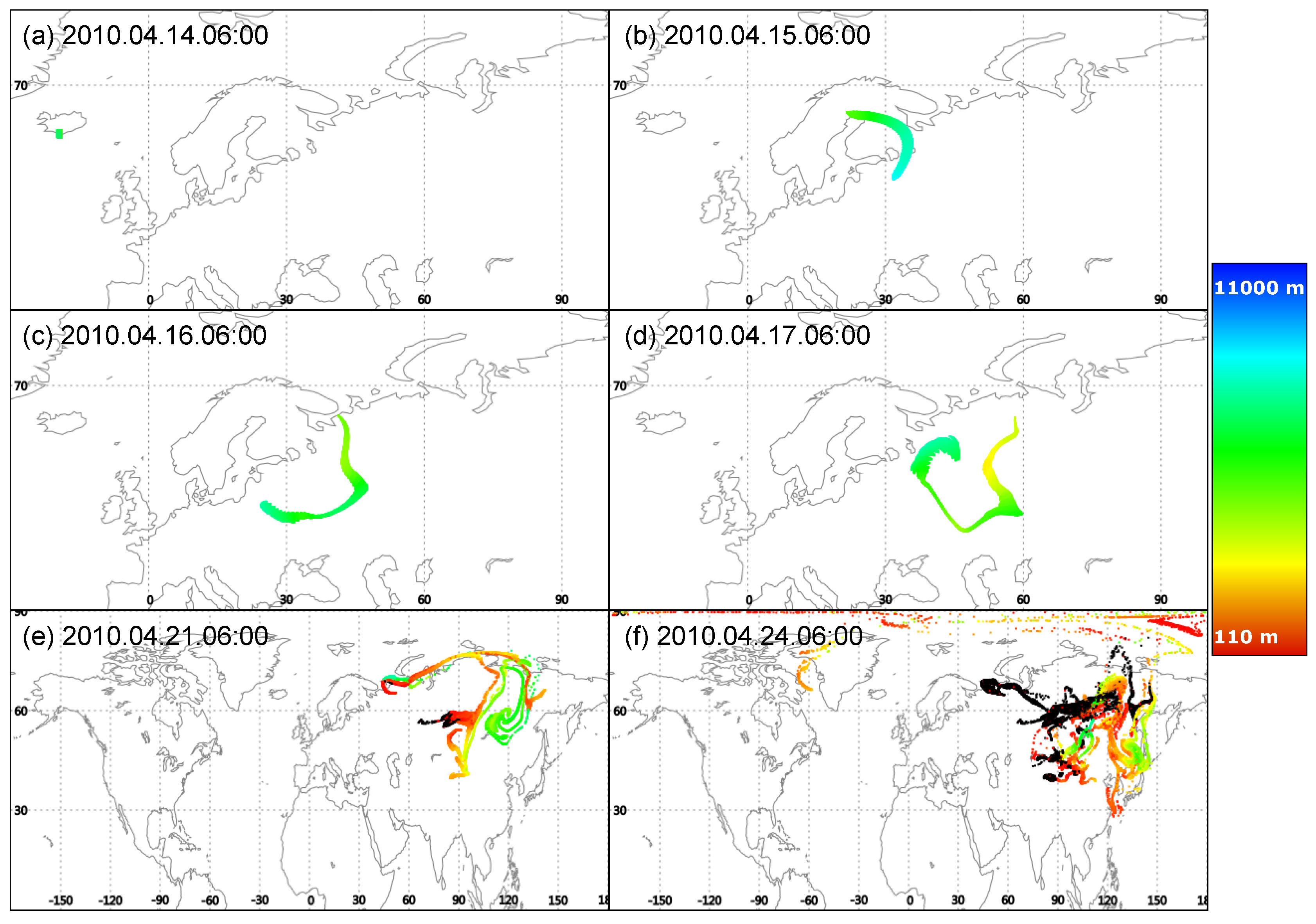
At the beginning (see Figure 1a), the top of the ash cloud reaches the altitude of 9 km (cyan color). However, due to the impact of gravity, the particles descend in the atmosphere more or less continuously (but not uniformly), and after two days they reach the altitude of about 4–6 km (green color, Figure 1c). Within three days, the altitude of the ash cloud in an extended region decreases even below 2–3 km (yellow color, Figure 1d). After 10 days a large number of particles are found to be deposited on the ground (black color, Figure 1f) across Siberia. The deposition distribution shows another important characteristic, typical of chaotic phenomena, namely that it is inhomogeneous with filamentary structure, with denser and sparser regions. Additionally, it can be also seen that particles do not fall out from the atmosphere at almost the same time as a coherent patch but rather some parts of the ash cloud are deposited by the 7th day after the eruption already (Figure 1e), while several particles are still in the middle of the troposphere, at an altitude of about 5 km (green) even after 10 days (Figure 1f). As it is introduced in Section 1, this kind of deposition dynamics is characteristic to transiently chaotic phenomena. The measure of the rapidity of deposition processes will be discussed in Section 4.3 in detail.
4.2. Stretching of the Pollutant Clouds—The Topological Entropy
Section 4.1 has shown that even an initially cuboid-shaped pollutant cloud soon becomes distorted into a tortuous, filamentary shape due to the chaotic nature of atmospheric spreading, and the extension of the cloud grows rapidly. To quantify this growth, by means of RePLaT-Chaos application, the time-dependence of the length increase of 1-D pollutant clouds (i.e., lines or filaments) can be measured. The stretching rate of the length, the topological entropy h in Equation (1), quantifies the intensity of the underlying chaotic dynamics which the pollutant cloud is subjected to during spreading.
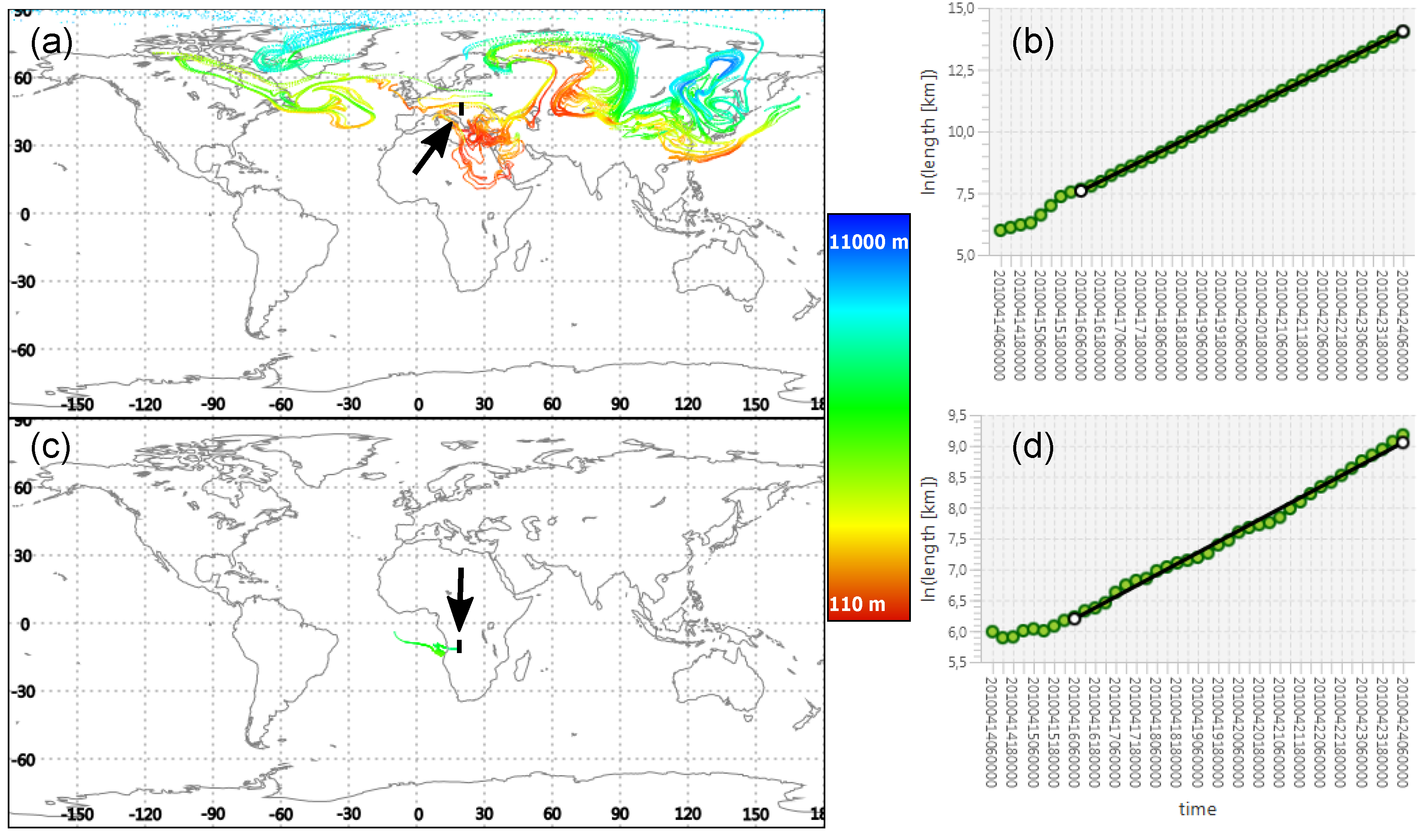
To get an impression of the meaning and consequences of the value of the topological entropy h, Figure 2 illustrates the distribution of two meridional line segments (having the same length at the emission) after 10 days and the corresponding curves of their length increase. Both cases show that the length of the filaments indeed grows in an approximately exponential manner in time (Figure 2b,d) after a few days (as a line in the semi-logarithmic plot). In Figure 2b the slope of the linear fit is day, while in Figure 2d the slope is found to be about 56% smaller, day. These values mean that in every and days the length of the pollutant cloud stretches by a factor of , respectively. With h being in the exponent in Equation (1), this approximately double factor between the topological entropies results in the fact that the length of the filaments after 10 days is about km for the filament initiated in Europe and km for the one emitted in Africa (calculated as and , respectively, reading the length data on April 24 at 6 UTC from the graphs.). The nearly 100-fold difference in their length (and the corresponding deviation of their topological entropies) obviously implies remarkably different distribution patterns at the end of the simulation. While day in Figure 2c is associated with a slightly crumpled filament which has not travelled far away from its initial location as it is drifting slowly with the trade winds near the Equatorial region, the filament in Figure 2a has a much more complicated shape with several foldings and meanders that cover a considerable part of the Northern Hemisphere. We note that, in general, larger topological entropy values and more intense spreading characterize the pollutant clouds initiated at the mid- and high latitudes than the ones start in the tropical region [30,31]. This is a consequence of the enhanced cyclonic activity in the extratropics associated with intensified shearing and mixing effects on the pollutant clouds. It is also worth noting that certain atmospheric features can be identified based on the pattern formed by the particles of the pollutant clouds: e.g., in Figure 2a south of Greenland and east of Scandinavia the trace of two cyclones can be noticed drawn by the spiral formations of the pollutant cloud.
4.3. Deposition of the Particles—The Escape Rate
Section 4.1 draws attention to the fact that the lifetime of particles even in an initially small pollutant cloud may be quite different. The reason behind the observed differences is that the particles do not fall directly purely vertically from their initial position onto the ground, but travel along complicated trajectories due to the chaotic nature of spreading. In this way their vertical movement is affected by both their terminal velocity and the local instantaneous vertical component of the air. Both the terminal velocity (Equation (5)) through kinematic viscosity and/or air density and the vertical air velocity v (Equation (5)) depend on the position of the particle and the time instant. For light aerosol particles the value of the upward directional vertical air velocity often exceeds the downward effect of their terminal velocity, thus, besides falling downwards on average, these particles have more chance to move also upwards in the atmosphere with the flows. The chaotic nature of spreading implies that nearby particles may reach remote locations within short times where they are also subjected to different vertical velocities, therefore, they may be deposited at considerably different time instants and locations.
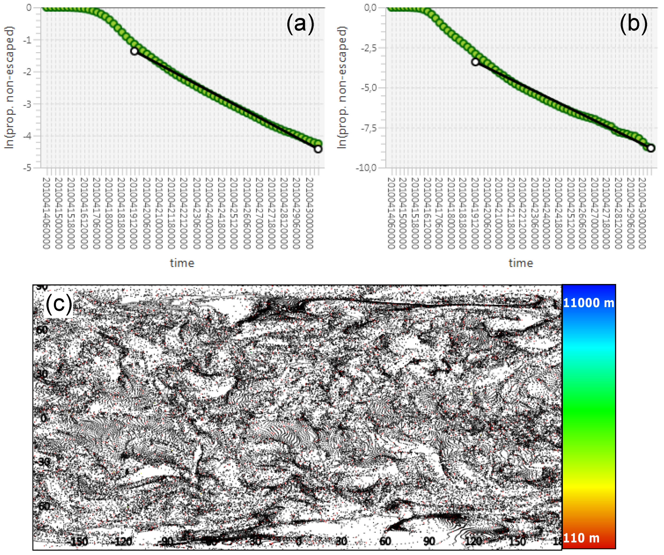
In order to study the process of deposition, Figure 3a,b shows how the ratio of non-deposited particles initially distributed uniformly over the globe at the altitude of 5.5 km changes in time. At the beginning of the simulation, a short plateau can be seen for both particles of radius m (Figure 3a) and m (Figure 3b), which indicates that a certain time is needed even for the “fastest falling” particles to reach the surface. After a short transient, the plateau is followed by an approximately exponential decrease in the ratio of non-escaped particles, the rapidity of which is characterized by the escape rate in Equation (2). The escape rate is smaller ( day) for smaller particles (Figure 3a) and larger ( day) for larger particles (Figure 3b), as expected naively, but it depends on the atmospheric conditions, too. In fact, the dependence of on r for m particles proved to be quadratic in a recent research studying aerosol particles with a realistic density of 2000 kg m [55]. This is in harmony with the fact that the updrafts and downdrafts in the atmosphere approximately balance each other’s effect on the particles, thus particles in rough average fall with their terminal velocity , which depended quadratically on r for these small particles with (Equation (5)). The obtained s imply that after the exponential decay takes place, after and days, only a proportion of of the particles can still be found in the air, respectively. It is worth noting that the reciprocal of is often considered to be a rough estimate of the average lifetime of typical particles in the exponentially decreasing stage [37,38].
Figure 3a,b also confirms an interesting observation made in Section 4.1 that even identical particles may often have significantly different lifetimes. For example, the first particles in Figure 3a leave the atmosphere on 15 April, only one day after the emission, while after more than two weeks, on 30 April, there are still 1.4% of the particles ( from the data of the graph) drifting in the atmosphere. Simulating the atmospheric spreading of a larger number of particles with m for a longer time period, it turns out that a ratio of – of the particles is able to survive more than two months in the atmosphere, as well as that the initial location of the long- and short-living particles folds into each other in thin filaments in a fractal structure in extended regions [55].
Figure 3c demonstrates that the inhomogeneity and irregularity in the pattern of the deposited particles in Figure 1f is not the consequence of the initially small extension of the volcanic ash cloud studied in Section 4.1. The filamentary deposition pattern with denser and sparser regions, typical for transient chaos, can also be seen even for particles initially distributed completely uniformly over the whole globe.
5. Conclusions
In this paper, the Lagrangian particle-tracking trajectory model RePLaT-Chaos is introduced and is shown to be applicable for the study of the main features of atmospheric pollutant spreading, which are also discussed in detail. Due to its user-friendly graphical user interface, RePLaT-Chaos is a suitable tool for anyone who is interested in studying the characteristics of the atmospheric spreading of pollutants. Users can design their own “volcano eruptions” changing the location, altitude, extent of the pollutant clouds, as well as the number of the tracked particles and their density and diameter. It can be easily observed how these parameters alter the spreading, and other interesting questions can also be studied, e.g.:
- How much faster do particles with larger size/higher density leave the atmosphere compared to smaller/lighter ones?
- Do the particles deposit on the surface in the shape of patches or in a filamentary structure?
- Is it possible for the particles of an initially small and compact pollutant cloud to cover more or less homogeneously the hemisphere where they are initialized, or the whole globe, and how long does it take?
- How does the initial geographical location of the pollutant clouds affect the rate of their stretching?
- Does the rapidity of the deposition or the stretching of a pollutant cloud depend on initialization time, e.g., the season in a year?
- Can cyclones, jet streams, etc. be revealed by tracking pollutant particles?
By means of RePLaT-Chaos, it can be easily shown that the spreading of volcanic ash and other atmospheric pollutants is peculiar, because it is an example of what is called a chaotic process. One can reveal that the basic difference between the dispersion of a dye droplet on clothes and the spreading of volcanic ash in the atmosphere is that the former grows slowly in a compact shape, while the latter becomes rapidly distorted into a filament, the length of which increases quickly in time. Furthermore, users can become acquainted with the basic concepts of chaos on their own. They experience the rapid divergence of nearby trajectories, the particles’ irregular motion in the atmosphere, and the above-mentioned quick development of pollutant clouds into a filamentary, tortuous and complicated but yet organized shape with many foldings and meanders.
Users can easily assign two quantities to their spreading events to characterize the chaotic behavior. One of them is the stretching rate of the pollutant clouds, the topological entropy: the greater its value the more quickly the length of the pollutant cloud grows, and the more foldings and complicated shape it has. Therefore, it can be considered as the measure of the strength of chaos and of the unpredictability of the spreading. The other eligible quantity, the escape rate, describes the rapidity of the approximately exponentially decaying process of particle deposition. Based on the graphs of the non-deposited particles, the users can observe on their own the quite different lifetimes of even identical aerosol particles injected into the atmosphere at very nearby geographic locations at the same time instant. In this way, RePLaT-Chaos can be considered as an educational reconstruction of results obtained from contemporary research regarding atmospheric spreading of pollutant clouds and chaotic advection.
As an outlook, we mention that RePLaT-Chaos has another version called RePLaT-Chaos-edu [64] with the same computational background and fewer simulation parameter options but with a more colorful user interface, designed especially for secondary school students. It is intended to serve as a tutorial about the main features of atmospheric pollutant spreading phenomenon. Therefore, besides allowing students to design their own pollution events, it includes a lot of eye-catching animations and easy-to-understand explanations in order to draw the students’ attention to the phenomena. The software was tested with a few group of students and received positive feedback [65].
Funding
This research was funded by the János Bolyai Research Scholarship of the Hungarian Academy of Sciences and by the National Research, Development and Innovation Office—NKFIH under grants PD-121305, PD-132709, FK-124256 and K-125171.
Acknowledgments
Fruitful discussions with T. Tél on chaotic advection and how to introduce it to students are gratefully acknowledged. The author thanks M. Herein and M. Vincze for testing the application, and G. Drotos, K. Klemm, M. Pinter and I. Takacs for suggestions on wording.
Conflicts of Interest
The author declares no conflict of interest.
Abbreviations
The following abbreviations are used in this manuscript:
| RePLaT | Real Particle Lagrangian Trajectory model |
Appendix A. RePLaT-Chaos Manual
Appendix A.1. First Steps and Data Format Requirements
Appendix A.1.1. Launching RePLaT-Chaos
RePLaT-Chaos can be downloaded from the website of the Institute for Theoretical Physics, Eötvös Loránd University [48]. Both a Windows executable installer file and a compressed file including a Java Archive application (usable also on Linux platforms) are accessible. In the former case, the installer installs the application in the folder RePLaT-Chaos in a user selected location. RePLaT-Chaos can be launched by clicking RePLaT-Chaos.exe in the folder. In the latter case the downloaded zip file should be unpacked, and the application can be launched, e.g., from the command prompt by typing the java -jar RePLaT-Chaos.jar command from folder RePLaT-Chaos. In both cases the folder RePLaT-Chaos has a sub-folder named default which contains the default values for the text fields of the user interface (default/default_*.txt files) and the continents.txt file for displaying the map for the simulations. Therefore, this folder and its contents should not be renamed or removed, however, the content of the default_*.txt files may be changed preserving their formats. Sample meteorological data in the required format are also available on the website for a 16-day time period overlapping with the Eyjafjallajökull volcano’s eruptions in 2010.
On the user interface the menu items and buttons with underlined letter/number can be reached not only by mouse clicks but also by keyboard shortcut Alt + <letter>/<number>.
Appendix A.1.2. Input Meteorological Data
For the simulation of the spreading of pollutant clouds meteorological data in Network Common Data Form (NetCDF) format files are needed. Data should be downloaded for the entire globe and at least six hours of time resolution. Such data are accessible in different temporal and spatial resolutions, e.g., from the European Center for Medium-Range Weather Forecasts (ECMWF) datasets [66] (ERA-40, ERA-Interim, etc.). The properties of the files required by RePLaT-Chaos are:
- Meteorological data on a regular longitude–latitude grid () at different pressure levels, where and are the horizontal grid resolutions. The software considers the lowest level as Earth’s surface and the highest one as the “top” of the simulation region.
- Required meteorological variables: zonal [m/s] and meridional [m/s] wind components, vertical velocity component [Pa/s] and temperature [K].
- A meteorological file contains the values of one of the meteorological variables on the above-mentioned grid for a single time instant.
- File name convention: <variable name><yyyyMMddhhmmss>.nc, where the format <yyyyMMddhhmmss> denotes the following: year (yyyy), month (MM), day (dd), hour (hh), minute (mm), second (ss) given in 4, 2, 2, 2, 2, and 2 digits, respectively.
Appendix A.1.3. Output Data
RePLaT-Chaos writes the data of the particles of the pollutant clouds to comma-separated values text files with CSV file extension, therefore, these files can be easily read or analyzed with other tools, too. An output file represents again a single time instant and contains one line for each particle. The file name convention is <file name pattern><yyyyMMddhhmmss>.csv. The comma separated data in a line are: , , z, r, , , where
- is the longitude coordinate of the particle [rad] ,
- is the latitude coordinate of the particle [rad] ,
- z is the vertical coordinate of the particle [m] calculated from its pressure coordinate p based on the equations of the standard atmosphere [67],
- r is the particle radius [m] ,
- is the particle density [kg m] ,
- represents whether the particle is in the atmosphere yet [1] or not [0].
The application computes the length of the pollutant cloud [km] and/or the ratio of the non-escaped particles if the user chooses this/these option(s). It writes the natural logarithms of these quantities to file at the time instants given by the user. The file of the length and the ratio of the non-escaped particles contain lines of format of <yyyyMMddhhmmss><tab>ln(value of the quantity).
Appendix A.2. Running a Simulation
In RePLaT-Chaos two setup options are available for a new simulation. In the first one parameters both for the simulation and for the pollutant cloud should be given. This screen is accessible via File menu clicking menu item New simulation—set parameters. The other options is New simulation—read parameters. In the latter case, pollutant clouds are not initialized according to user-given parameters rather its particles are read from a file.
Appendix A.2.1. Setting the Simulation Parameters
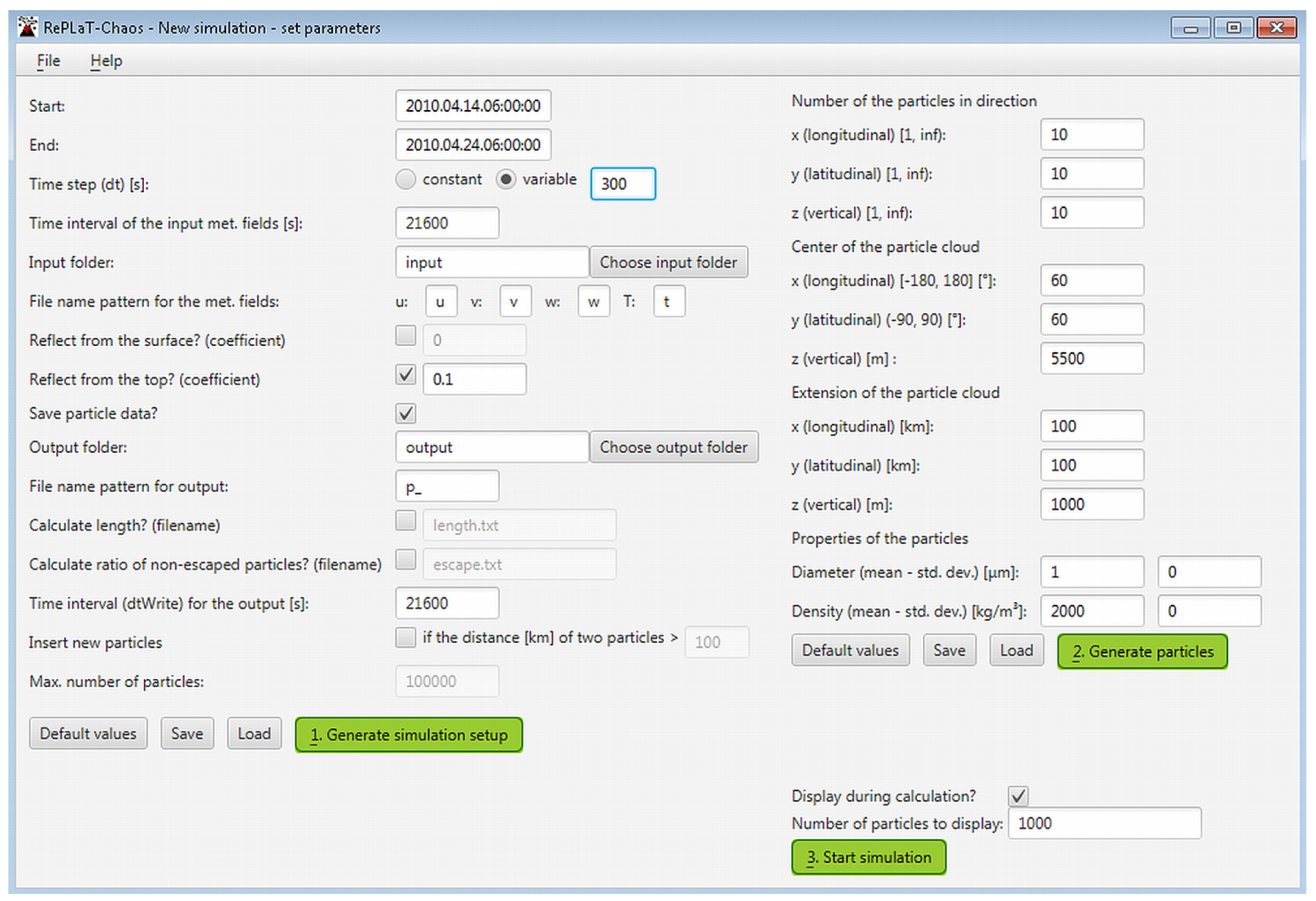
The user chooses either the New simulation—set parameters or the New simulation—read parameters menu item, in both cases the simulation parameters should be given at first (left panel of the screen in Figure A1 and Figure A2). These parameters are the following:
- Start: start date and time of the simulation (format: <yyyy.MM.dd.hh:mm:ss>).
- End: end date and time of the simulation (format: <yyyy.MM.dd.hh:mm:ss>).
- Time step: if it is constant then the text field represents the value of the constant time step [s] (format: integer); if it is variable then the text field corresponds to defined in Section 3.1.
- Input folder: folder of the meteorological files. Clicking the Choose input folder button it can be chosen or it can be written directly to the text field.
- File name pattern for the met. fields: the part of the file name before date and time for the meteorological files of the zonal (u), meridional (v), vertical (w) velocity component of air and the temperature (T).
- Reflect from the surface?: if the box is checked each particle bounces back from the lowest meteorological level according to the Reflection coefficient for the surface (format: real). For topological entropy (length) calculation, the box is worth checking and 1 should be given for the reflection coefficient.
- Reflect from the top?: if the box is checked each particle bounces back from the highest meteorological level according to the Reflection coefficient for the top (format: real). Generally, the box is worth checking unless the user especially wants to study how many particles leave the meteorological region at the highest level.
- Save particle data?: should the data of the particles of the pollutant cloud (and the length data and the ratio of the non-escaped particles) be written to file. For example, user should not check the box if he/she carries out test calculations and would like to see the spreading of pollutant cloud only once, i.e., when the user does not need the data later.
- Output folder: the folder of the files for particle data, length data and ratio of the non-escaped particles. Clicking the Choose output folder button it can be chosen or it can be written directly to the text field.
- File name pattern for the output: the part of the particle data file name before date and time.
- Calculate length? (filename): should the length of the pollutant cloud be calculated, and if yes, what should be the name of the length file to which the data are written. The length of the pollutant cloud is computed as the sum of the distances between the subsequent particles as described in Section 3.2. Therefore, the result of the calculation equals to the real length in the unit of km only if the particles are initiated as a one-dimensional “pollutant cloud”, i.e, a line segment.
- Calculate ratio of non-escaped particles? (filename): should the ratio of the non-escaped particles be calculated, and if yes, what should be the name of the escape file to which the data are written.
- Time interval for the output: the time interval [s] for writing the data of the pollutant cloud, of the length and of the ratio of the non-escaped particles to file (format: integer)
- Insert new particles if the distance [km] of two particles: should new particles be inserted in the pollutant cloud if the distance of two subsequent particles is greater than the given distance (format: real). The box is worth checking for length calculation; otherwise subsequent particles may travel far away from each other which results in the underestimation of the length of the pollutant cloud as described in Section 3.2.
- Max. number of particles: The number of the particles in the simulation, including the inserted ones, does not exceed the given number (format: integer).
By default, the fields are filled with the default setting parameters loaded from default/ default_simulation_setup.txt. After overwriting any field, the user can reload the default values by clicking the Default button, new data can be loaded in the fields from a chosen file by clicking the Load button, or the values of the fields can be saved in a new file by clicking the Save button. If there is a wrong or empty text field, data could not be saved: the problem is indicated by an alert window.
At first, for starting a simulation the generation of the simulation setup is required: the user can generate it by clicking the Generate simulation setup button. If there is a wrong or empty text field, similarly to saving, the problem is indicated by an alert window. If there is no wrong or empty text field, a pop-up window indicates that the Simulation setup is generated. Then the disabled right panel (the parameter settings of the pollutant cloud (Figure A1) or the data for reading particles of a pollutant cloud (Figure A2)) becomes enabled.
Figure A1.
New simulation—set parameters. Starting a new simulation by setting the parameters of the simulation and the pollutant cloud.
Figure A1.
New simulation—set parameters. Starting a new simulation by setting the parameters of the simulation and the pollutant cloud.

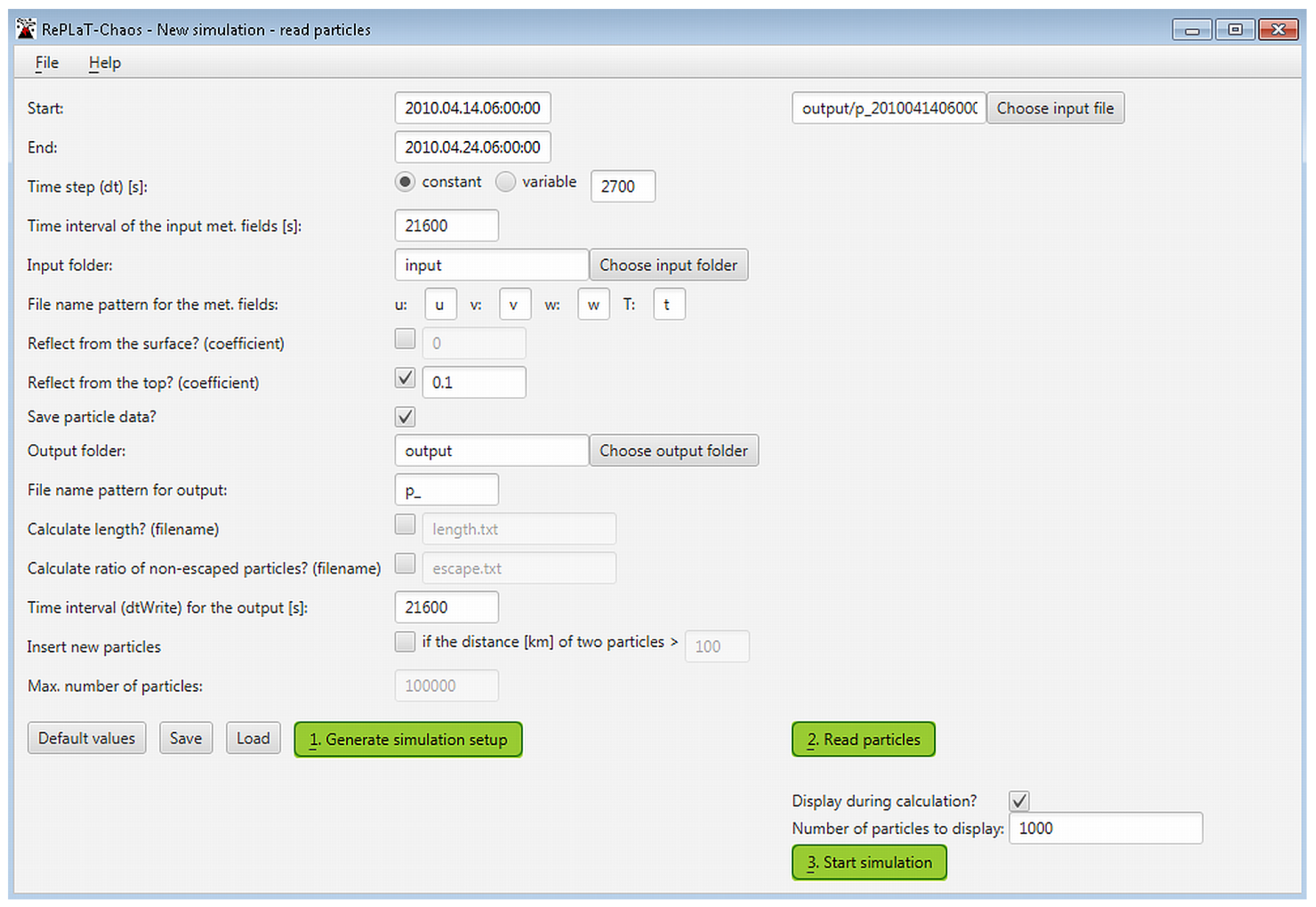
Figure A2.
New simulation - read particles. Starting a new simulation by setting the parameters of the simulation and reading the particles of the pollutant clouds from file.
Figure A2.
New simulation - read particles. Starting a new simulation by setting the parameters of the simulation and reading the particles of the pollutant clouds from file.

Appendix A.2.2. Setting the Parameters of the Pollutant Cloud
In case of choosing the New simulation—set parameters option (Figure A1) the user should set the following parameters of the particles which will fill a rectangular cuboid:
- Number of particles in direction x/y/z: the number of the particles in zonal, meridional and vertical direction (format: integers, greater or equal than 1).
- Center of the particle cloud x/y/z: zonal [], meridional [] and vertical [m] coordinate of the center of the pollutant cloud (format: real numbers in the given intervals)
- Extension of the particle cloud x/y/z: length of the sides of the rectangular cuboid representing the pollutant cloud in zonal [km], meridional [km] and vertical [m] direction (format: non-negative real)
- Diameter (mean–std.dev.): the diameter of the particles is log-normally distributed with the user given mean and standard deviation [m] (format: non-negative real). As mentioned in Section 3.1, the diameter 0 m corresponds to gas particles which are advected by the instantaneous velocity of the atmospheric flow at each time instant (their terminal velocity in Equation (5) is 0).
- Density (mean–std.dev.): the density of the particles is log-normally distributed with the user given mean and standard deviation [kg m] (format: non-negative real).
By default, the fields are filled with the default setting parameters loaded from default/ default_particle_parameter_setup.txt. The usage of the Default, Save and Load buttons are analogous to the ones in the simulation setup panel.
For starting a simulation the generation of the pollutant cloud is required: the user can generate it by clicking the Generate particles button. If there is a wrong or empty text field, the problem is indicated by an alert window. Otherwise a pop-up window indicates that the pollutant cloud is generated (Number of particles: <particle number>.). Then the disabled bottom right panel (for setting the display properties of the simulation and starting the simulation calculation (Figure A1)) becomes enabled.
Appendix A.2.3. Reading the Particles of the Pollutant Cloud From File
In the case of reading the particles of the pollutant cloud (Figure A2), the user chooses the file containing the initial conditions of its particles by clicking the Choose input file button. The default file path is in the file default/default_particle_file_setup.txt. The formats and the values of data in the file should meet the requirements which are listed in Appendix A.1.3. The particle data are read from the file by clicking the Read particles button. In the case of wrong values an alert window indicates the problem: There were invalid data while reading from file <file> <wrong lines>. If every line is correct, a pop-up window indicates that the pollutant cloud is generated (Number of particles: <particle number>.). Then the disabled bottom right panel (for setting the display properties of the simulation and starting the simulation calculation (Figure A2)) becomes enabled.
This way of generating a pollutant cloud is worth applying when the user does not want to initialize the particles filling a rectangular cuboid (mentioned in the previous section) rather than the user needs particles with arbitrary positions. For example, in this way several different particle groups (i.e., different pollutant clouds) initialized at different locations can be tracked simultaneously.
Appendix A.2.4. Starting a New Simulation
In the bottom right panel (Figure A1 and Figure A2) the user should check whether if she/he wants to watch the spreading of the pollutant cloud during the simulation calculation (Display during calculation?) and if yes, how many particles of the pollutant cloud should be drawn (Number of particles to display, format: integer). By clicking the Start simulation button the simulation calculation starts and the progress (and the particle cloud if chosen) can be tracked in a new window (Figure A3).
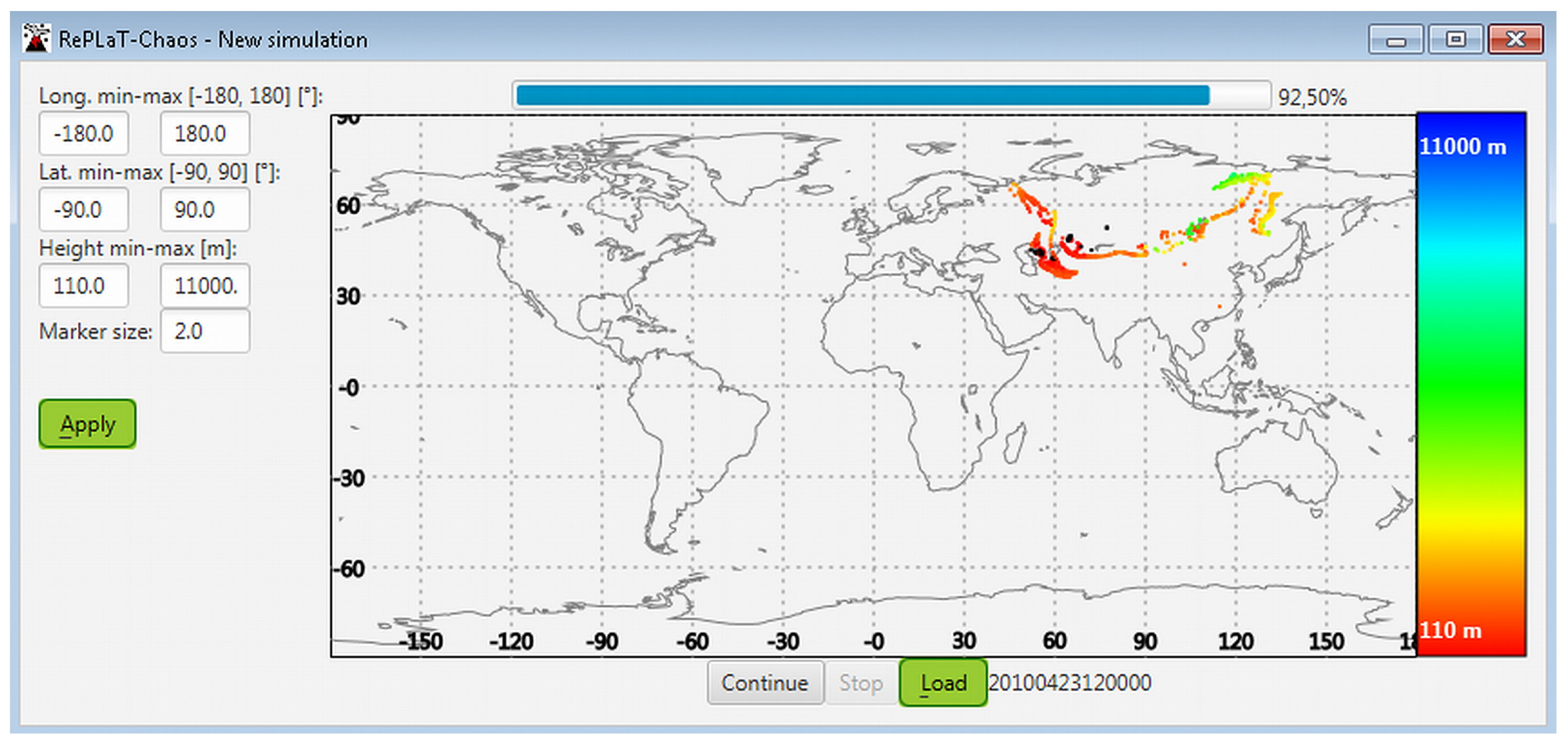
Figure A3.
Example for tracking the calculation of the simulation with displaying the particle positions. The simulation and the pollutant cloud are initialized with the parameters in Figure A1. The colorbar indicates the altitude of the particles.
Figure A3.
Example for tracking the calculation of the simulation with displaying the particle positions. The simulation and the pollutant cloud are initialized with the parameters in Figure A1. The colorbar indicates the altitude of the particles.

Appendix A.2.5. Setting the Display Properties of the Simulation
If the user has chosen the display option, the position of the particles of the pollutant cloud is displayed continuously colored according to the vertical coordinate of the particles on a map (Figure A3) during the simulation calculation. Otherwise only a progressbar is visible to show the percentage of the progress of the calculation and the corresponding date and time in the simulation. The user can stop and continue the calculation by clicking the Stop or Continue buttons, respectively, and she/he can load the particle data saved in files for replay by clicking the Load button. The longitudinal and latitudinal boundaries of the map, the vertical boundaries of the coloring and the marker size of the particles can be changed on the left side (formats: real numbers in the given intervals). The settings are applied by clicking the Apply button. If there is a wrong or empty text field, the problem is indicated by an alert window.
Appendix A.3. Replaying a Saved Simulation
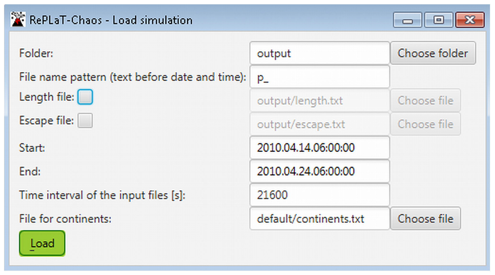
A saved simulation can be loaded by clicking the Load simulation menu item in File menu on the new simulation screen or by clicking the Load button in the case of an ongoing simulation. Then the parameters defining the saved simulation appear in a new window (Figure A4). For ongoing simulation text fields are filled with the parameters of the simulation, otherwise they are filled with the values loaded from the default/default_load_setup.txt. The following parameters should be given:
- Folder: folder of the files to be loaded. Clicking the Choose folder button it can be chosen or it can be written directly to the text field.
- File name pattern: the part of the name of the particle files before date and time.
- Length file: should length data be loaded, and if yes from which file. Clicking the Choose file button it can be chosen or it can be written directly to the text field.
- Escape file: should the data of the ratio of non-escaped particles be loaded, and if yes from which file. Clicking the Choose file button it can be chosen or it can be written directly to the text field. The format of the lines of the length and escape file should coincide with the requirements mentioned in Appendix A.1.3.
- Start: start of the display (format: <yyyy.MM.dd.hh:mm:ss>)
- End: end of the display (format: <yyyy.MM.dd.hh:mm:ss>)
- Time interval of the input files: time interval [s] between subsequent files to be displayed (format: integer)
- File for continents: the file which contains the coordinates ( [rad]) of the coastlines of the continents. Clicking the Choose file button it can be chosen, or it can be written directly to the text field.
Figure A4.
Setting simulation data for loading saved simulation.

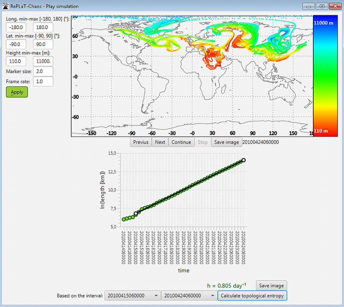
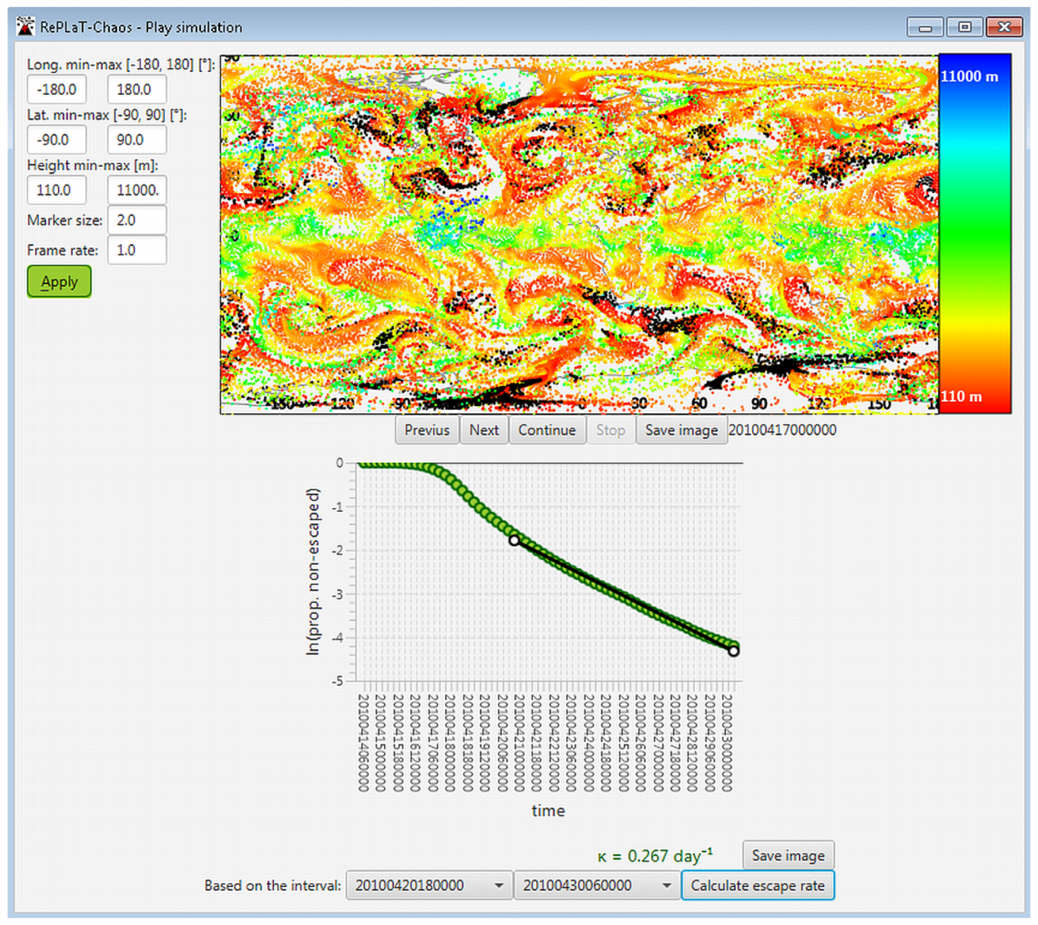
The selected simulation is loaded by clicking the Load button. If the Length file/Escape file is checked, the time dependence of the natural logarithm of the length of the pollutant cloud/the time dependence of the natural logarithm of the ratio of the non-escaped particles also appears on the display panel (Figure A5 and Figure A6). By default, the forward loop of the spreading of pollutant cloud is displayed according to the given Frame rate. The user can stop (Stop) and continue (Continue) the replay, and can move frame by frame the replay forward/backward by clicking the Previous/Next buttons. The instantaneous position of the pollutant cloud can be saved as an image by the Save image button. The properties of the display can be changed similarly as described in Appendix A.2.5 by clicking the Apply button. Beyond those options the speed of the animation (Frame rate) can be modified, too.
If the user has loaded length data/data for the ratio of the non-escaped particles from file, she/he can select a start and end date and time from two lists in the bottom of the panel in Figure A5 or Figure A6. By clicking the Calculate topological entropy/Calculate escape rate button a line is fitted to the graph between the given time instants using the least squares approach (Section 3.2 and Section 3.3) and its slope (i.e., the topological entropy h (Figure A5))/ slope (i.e., the escape rate (Figure A6)) appears. The value of the obtained topological entropy h in Figure A5 means that in every days the length of the pollutant cloud stretches by a factor of . Analogously, the value of the escape rate in Figure A6 implies that within days after the start time of the fit only of the particles (which are non-escaped at the start time of the fit) are still in the air. The graphs can be saved by clicking the Save image button.
Figure A5.
Displaying saved simulation and the time dependence of the length of a pollutant cloud. The simulation is initialized with the simulation parameters on the left of Figure A1 but with top and bottom reflection coefficients of 1 and inserting new particles if the distance of two particles is greater than 100 km. The pollutant cloud is initialized as a meridional line segment of 400 km at 47 N, 19 E and at the altitude of 5500 m. It consists of 1000 particles at the beginning. The particle radius is 0 m.

Figure A6.
Displaying saved simulation and the time dependence of the ratio of non-escaped particles. The simulation is initialized with the simulation parameters on the left of Figure A1 but with an end date of “2010.04.30.06:00:00” and with calculating the ratio of non-escaped particles. The pollutant cloud is initialized as particles at 0 N, 0 E and at the altitude of 5500 m with an extension of (i.e., covering the entire globe uniformly). The particle radius and density is 7 m and 2000 kg m, respectively.

References
- Ulfarsson, G.F.; Unger, E.A. Impacts and Responses of Icelandic Aviation to the 2010 Eyjafjallajökull Volcanic Eruption: Case Study. Transp. Res. Rec. 2011, 2214, 144–151. [Google Scholar] [CrossRef]
- Wilkinson, S.M.; Dunn, S.; Ma, S. The vulnerability of the European air traffic network to spatial hazards. Nat. Hazards 2012, 60, 1027–1036. [Google Scholar] [CrossRef] [Green Version]
- Arason, P.; Petersen, G.; Bjornsson, H. Observations of the altitude of the volcanic plume during the eruption of Eyjafjallajökull, April–May 2010. Earth Syst. Sci. Data 2011, 3, 9–17. [Google Scholar] [CrossRef] [Green Version]
- Stohl, A.; Prata, A.; Eckhardt, S.; Clarisse, L.; Durant, A.; Henne, S.; Kristiansen, N.I.; Minikin, A.; Schumann, U.; Seibert, P.; et al. Determination of time-and height-resolved volcanic ash emissions and their use for quantitative ash dispersion modeling: The 2010 Eyjafjallajökull eruption. Atmos. Chem. Phys. 2011, 11, 4333–4351. [Google Scholar] [CrossRef] [Green Version]
- Schumann, U.; Weinzierl, B.; Reitebuch, O.; Schlager, H.; Minikin, A.; Forster, C.; Baumann, R.; Sailer, T.; Graf, K.; Mannstein, H.; et al. Airborne observations of the Eyjafjalla volcano ash cloud over Europe during air space closure in April and May 2010. Atmos. Chem. Phys. 2011, 11, 2245–2279. [Google Scholar] [CrossRef] [Green Version]
- Sicard, M.; Guerrero-Rascado, J.L.; Navas-Guzmán, F.; Preißler, J.; Molero, F.; Tomás, S.; Bravo-Aranda, J.A.; Comerón, A.; Rocadenbosch, F.; Wagner, F.; et al. Monitoring of the Eyjafjallajökull volcanic aerosol plume over the Iberian Peninsula by means of four EARLINET lidar stations. Atmos. Chem. Phys. 2012, 12, 3115–3130. [Google Scholar] [CrossRef] [Green Version]
- Pappalardo, G.; Mona, L.; D’Amico, G.; Wandinger, U.; Adam, M.; Amodeo, A.; Ansmann, A.; Apituley, A.; Alados Arboledas, L.; Balis, D.; et al. Four-dimensional distribution of the 2010 Eyjafjallajökull volcanic cloud over Europe observed by EARLINET. Atmos. Chem. Phys. 2013, 13, 4429–4450. [Google Scholar] [CrossRef] [Green Version]
- Burlakov, V.; Dolgii, S.; Nevzorov, A.; Samokhvalov, I.; Nasonov, S.; Zhivotenyuk, I.; El’nikov, A.; Nazarov, E.; Plusnin, I.; Shikhantsov, A. Traces of eruption of Eyjafjallajökull volcano according to data of lidar observations in Tomsk and Surgut. Atmos. Ocean. Opt. 2012, 25, 110–117. [Google Scholar] [CrossRef]
- Zuev, V.V.; Burlakov, V.D.; Nevzorov, A.V.; Pravdin, V.L.; Savelieva, E.S.; Gerasimov, V.V. 30-year lidar observations of the stratospheric aerosol layer state over Tomsk (Western Siberia, Russia). Atmos. Chem. Phys. 2017, 17, 3067–3081. [Google Scholar] [CrossRef] [Green Version]
- Petersen, G.; Bjornsson, H.; Arason, P.; Löwis, S.V. Two weather radar time series of the altitude of the volcanic plume during the May 2011 eruption of Grímsvötn, Iceland. Earth Syst. Sci. Data 2012, 4, 121–127. [Google Scholar] [CrossRef] [Green Version]
- Tesche, M.; Glantz, P.; Johansson, C.; Norman, M.; Hiebsch, A.; Ansmann, A.; Althausen, D.; Engelmann, R.; Seifert, P. Volcanic ash over Scandinavia originating from the Grímsvötn eruptions in May 2011. J. Geophys. Res. Atmos. 2012, 117. [Google Scholar] [CrossRef]
- Wilkins, K.; Western, L.; Watson, I. Simulating atmospheric transport of the 2011 Grímsvötn ash cloud using a data insertion update scheme. Atmos. Environ. 2016, 141, 48–59. [Google Scholar] [CrossRef] [Green Version]
- Bowyer, T.W.; Biegalski, S.R.; Cooper, M.; Eslinger, P.W.; Haas, D.; Hayes, J.C.; Miley, H.S.; Strom, D.J.; Woods, V. Elevated radioxenon detected remotely following the Fukushima nuclear accident. J. Environ. Radioact. 2011, 102, 681–687. [Google Scholar] [CrossRef] [PubMed]
- Leon, J.D.; Jaffe, D.; Kaspar, J.; Knecht, A.; Miller, M.; Robertson, R.; Schubert, A. Arrival time and magnitude of airborne fission products from the Fukushima, Japan, reactor incident as measured in Seattle, WA, USA. J. Environ. Radioact. 2011, 102, 1032–1038. [Google Scholar] [CrossRef] [PubMed] [Green Version]
- MacMullin, S.; Giovanetti, G.; Green, M.; Henning, R.; Holmes, R.; Vorren, K.; Wilkerson, J. Measurement of airborne fission products in Chapel Hill, NC, USA from the Fukushima Dai-ichi reactor accident. J. Environ. Radioact. 2012, 112, 165–170. [Google Scholar] [CrossRef] [PubMed] [Green Version]
- Masson, O.; Baeza, A.; Bieringer, J.; Brudecki, K.; Bucci, S.; Cappai, M.; Carvalho, F.; Connan, O.; Cosma, C.; Dalheimer, A.; et al. Tracking of airborne radionuclides from the damaged Fukushima Dai-ichi nuclear reactors by European networks. Environ. Sci. Technol. 2011, 45, 7670–7677. [Google Scholar] [CrossRef]
- Bossew, P.; Kirchner, G.; De Cort, M.; De Vries, G.; Nishev, A.; De Felice, L. Radioactivity from Fukushima Dai-ichi in air over Europe; part 1: Spatio-temporal analysis. J. Environ. Radioact. 2012, 114, 22–34. [Google Scholar] [CrossRef]
- Stohl, A.; Seibert, P.; Wotawa, G.; Arnold, D.; Burkhart, J.; Eckhardt, S.; Tapia, C.; Vargas, A.; Yasunari, T. Xenon-133 and caesium-137 releases into the atmosphere from the Fukushima Dai-ichi nuclear power plant: Determination of the source term, atmospheric dispersion, and deposition. Atmos. Chem. Phys. 2012, 12, 2313–2343. [Google Scholar] [CrossRef] [Green Version]
- Manolopoulou, M.; Vagena, E.; Stoulos, S.; Ioannidou, A.; Papastefanou, C. Radioiodine and radiocesium in Thessaloniki, Northern Greece due to the Fukushima nuclear accident. J. Environ. Radioact. 2011, 102, 796–797. [Google Scholar] [CrossRef]
- Pittauerová, D.; Hettwig, B.; Fischer, H.W. Fukushima fallout in Northwest German environmental media. J. Environ. Radioact. 2011, 102, 877–880. [Google Scholar] [CrossRef]
- Bikit, I.; Mrda, D.; Todorovic, N.; Nikolov, J.; Krmar, M.; Veskovic, M.; Slivka, J.; Hansman, J.; Forkapic, S.; Jovancevic, N. Airborne radioiodine in northern Serbia from Fukushima. J. Environ. Radioact. 2012, 114, 89–93. [Google Scholar] [CrossRef] [PubMed]
- Castruccio, A.; Clavero, J.; Segura, A.; Samaniego, P.; Roche, O.; Le Pennec, J.L.; Droguett, B. Eruptive parameters and dynamics of the April 2015 sub-Plinian eruptions of Calbuco volcano (southern Chile). Bull. Volcanol. 2016, 78, 62. [Google Scholar] [CrossRef]
- Romero, J.; Morgavi, D.; Arzilli, F.; Daga, R.; Caselli, A.; Reckziegel, F.; Viramonte, J.; Díaz-Alvarado, J.; Polacci, M.; Burton, M.; et al. Eruption dynamics of the 22–23 April 2015 Calbuco Volcano (Southern Chile): Analyses of tephra fall deposits. J. Volcanol. Geotherm. Res. 2016, 317, 15–29. [Google Scholar] [CrossRef] [Green Version]
- Reckziegel, F.; Bustos, E.; Mingari, L.; Báez, W.; Villarosa, G.; Folch, A.; Collini, E.; Viramonte, J.; Romero, J.; Osores, S. Forecasting volcanic ash dispersal and coeval resuspension during the April–May 2015 Calbuco eruption. J. Volcanol. Geotherm. Res. 2016, 321, 44–57. [Google Scholar] [CrossRef] [Green Version]
- Ivy, D.J.; Solomon, S.; Kinnison, D.; Mills, M.J.; Schmidt, A.; Neely, R.R. The influence of the Calbuco eruption on the 2015 Antarctic ozone hole in a fully coupled chemistry-climate model. Geophys. Res. Lett. 2017, 44, 2556–2561. [Google Scholar] [CrossRef]
- Corsaro, R.A.; Andronico, D.; Behncke, B.; Branca, S.; Caltabiano, T.; Ciancitto, F.; Cristaldi, A.; De Beni, E.; La Spina, A.; Lodato, L.; et al. Monitoring the December 2015 summit eruptions of Mt. Etna (Italy): Implications on eruptive dynamics. J. Volcanol. Geotherm. Res. 2017, 341, 53–69. [Google Scholar] [CrossRef]
- Pompilio, M.; Bertagnini, A.; Del Carlo, P.; Di Roberto, A. Magma dynamics within a basaltic conduit revealed by textural and compositional features of erupted ash: The December 2015 Mt. Etna paroxysms. Sci. Rep. 2017, 7, 4805. [Google Scholar] [CrossRef]
- Athanassiadou, M. The Mt Etna SO2 eruption in December 2015—The view from space. Weather 2016, 71, 273–279. [Google Scholar] [CrossRef]
- Haszpra, T.; Tél, T. Escape rate: A Lagrangian measure of particle deposition from the atmosphere. Nonlinear Process. Geophys. 2013, 20, 867–881. [Google Scholar] [CrossRef] [Green Version]
- Haszpra, T.; Herein, M. Ensemble-based analysis of the pollutant spreading intensity induced by climate change. Sci. Rep. 2019, 9, 3896. [Google Scholar] [CrossRef] [Green Version]
- Haszpra, T.; Tél, T. Topological entropy: A Lagrangian measure of the state of the free atmosphere. J. Atmos. Sci. 2013, 70, 4030–4040. [Google Scholar] [CrossRef] [Green Version]
- Dutton, E.G.; Christy, J.R. Solar radiative forcing at selected locations and evidence for global lower tropospheric cooling following the eruptions of El Chichon and Pinatubo. Geophys. Res. Lett. 1992, 19, 2313–2316. [Google Scholar] [CrossRef]
- Kerr, R.A. Pinatubo global cooling on target. Science 1993, 259, 594–595. [Google Scholar]
- Self, S.; Zhao, J.X.; Holasek, R.E.; Torres, R.C.; King, A.J. The atmospheric impact of the 1991 Mount Pinatubo eruption. In Fire and Mud: The Eruptions and Lahars of Mount Pinatubo, Philippines; Newhall, C.G., Punongbayan, R., Eds.; University of Washington Press: Seattle, WA, USA, 1996; pp. 1089–1116. [Google Scholar]
- Ott, E. Chaos in Dynamical Systems; Cambridge University Press: New York, NY, USA, 1993; p. 385. [Google Scholar]
- Tél, T.; Gruiz, M. Chaotic Dynamics: An Introduction Based on Classical Mechanics; Cambridge University Press: Cambridge, UK, 2006; p. 393. [Google Scholar]
- Lai, Y.C.; Tél, T. Transient Chaos: Complex Dynamics on Finite Time Scales; Springer-Verlag New York: New York, NY, USA, 2011; Volume 173. [Google Scholar]
- Tél, T. The joy of transient chaos. Chaos Interdiscip. J. Nonlinear Sci. 2015, 25, 097619. [Google Scholar] [CrossRef]
- Haszpra, T. Intensification of Large-Scale Stretching of Atmospheric Pollutant Clouds due to Climate Change. J. Atmos. Sci. 2017, 74, 4229–4240. [Google Scholar] [CrossRef]
- Stein, A.; Draxler, R.R.; Rolph, G.D.; Stunder, B.J.; Cohen, M.; Ngan, F. NOAA’s HYSPLIT atmospheric transport and dispersion modeling system. Bull. Am. Meteorol. Soc. 2015, 96, 2059–2077. [Google Scholar] [CrossRef]
- Rolph, G.; Stein, A.; Stunder, B. Real-time environmental applications and display sYstem: READY. Environ. Model. Softw. 2017, 95, 210–228. [Google Scholar] [CrossRef]
- Miltenberger, A.K.; Pfahl, S.; Wernli, H. An online trajectory module (version 1.0) for the nonhydrostatic numerical weather prediction model COSMO. Geosci. Model Dev. 2013, 6, 1989–2004. [Google Scholar] [CrossRef] [Green Version]
- Sprenger, M.; Wernli, H. The LAGRANTO Lagrangian analysis tool—Version 2.0. Geosci. Model Dev. 2015, 8, 2569–2586. [Google Scholar] [CrossRef] [Green Version]
- Pisso, I.; Sollum, E.; Grythe, H.; Kristiansen, N.; Cassiani, M.; Eckhardt, S.; Arnold, D.; Morton, D.; Thompson, R.L.; Groot Zwaaftink, C.D.; et al. The Lagrangian particle dispersion model FLEXPART version 10.3. Geosci. Model Dev. Discuss. 2019, 2019, 1–67. [Google Scholar] [CrossRef] [Green Version]
- Costa, A.; Macedonio, G.; Folch, A. A three-dimensional Eulerian model for transport and deposition of volcanic ashes. Earth Planet. Sci. Lett. 2006, 241, 634–647. [Google Scholar] [CrossRef]
- Folch, A.; Costa, A.; Macedonio, G. FALL3D: A computational model for volcanic ash transport and deposition. Comput. Geosci. 2009, 35, 1334–1342. [Google Scholar] [CrossRef]
- Folch, A.; Costa, A.; Macedonio, G. FPLUME-1.0: An integral volcanic plume model accounting for ash aggregation. Geosci. Model Dev. 2016, 9, 431–450. [Google Scholar] [CrossRef] [Green Version]
- RePLaT-Chaos. Available online: http://theorphys.elte.hu/fiztan/volcano/#full (accessed on 21 December 2019).
- Chandler, M.A.; Richards, S.J.; Shopsin, M. EdGCM: Enhancing climate science education through climate modeling research projects. In Proceedings of the 85th Annual Meeting of the American Meteorological Society, 14th Symposium on Education, San Diego, CA, USA, 8–14 January 2005; p. P1. [Google Scholar]
- Fraedrich, K.; Jansen, H.; Kirk, E.; Luksch, U.; Lunkeit, F. The Planet Simulator: Towards a user friendly model. Meteorol. Z. 2005, 14, 299–304. [Google Scholar] [CrossRef]
- Newhouse, S.; Pignataro, T. On the estimation of topological entropy. J. Stat. Phys. 1993, 72, 1331–1351. [Google Scholar] [CrossRef]
- Thiffeault, J.L. Braids of entangled particle trajectories. Chaos 2010, 20, 017516. [Google Scholar] [CrossRef] [Green Version]
- Budišić, M.; Thiffeault, J.L. Finite-time braiding exponents. Chaos 2015, 25, 087407. [Google Scholar] [CrossRef] [Green Version]
- Haszpra, T.; Horányi, A. Some aspects of the impact of meteorological forecast uncertainties on environmental dispersion prediction. Idojaras 2014, 118, 335–347. [Google Scholar]
- Haszpra, T. Intricate features in the lifetime and deposition of atmospheric aerosol particles. Chaos Interdiscip. J. Nonlinear Sci. 2019, 29, 071103. [Google Scholar] [CrossRef]
- Haszpra, T.; Tél, T. Volcanic ash in the free atmosphere: A dynamical systems approach. In Journal of Physics: Conference Series; IOP Publishing: Bristol, UK, 2011; Volume 333, p. 012008. [Google Scholar]
- Haszpra, T.; Tél, T. Individual particle based description of atmospheric dispersion: A dynamical systems approach. In The Fluid Dynamics of Climate; Springer-Verlag Wien: Wien, Austria, 2016; pp. 95–119. [Google Scholar]
- Sutherland, W. LII. The viscosity of gases and molecular force. Philos. Mag. Ser. 1893, 36, 507–531. [Google Scholar] [CrossRef] [Green Version]
- Stohl, A.; Wotawa, G.; Seibert, P.; Kromp-Kolb, H. Interpolation errors in wind fields as a function of spatial and temporal resolution and their impact on different types of kinematic trajectories. J. Appl. Meteorol. 1995, 34, 2149–2165. [Google Scholar] [CrossRef] [Green Version]
- Flentje, H.; Claude, H.; Elste, T.; Gilge, S.; Köhler, U.; Plass-Dülmer, C.; Steinbrecht, W.; Thomas, W.; Werner, A.; Fricke, W. The Eyjafjallajökull eruption in April 2010–detection of volcanic plume using in-situ measurements, ozone sondes and lidar-ceilometer profiles. Atmos. Chem. Phys. 2010, 10, 10085–10092. [Google Scholar] [CrossRef] [Green Version]
- Belosi, F.; Santachiara, G.; Prodi, F. Eyjafjallajökull volcanic eruption: Ice nuclei and particle characterization. Atmos. Clim. Sci. 2011, 1, 48. [Google Scholar]
- Campanelli, M.; Estelles, V.; Smyth, T.; Tomasi, C.; Martìnez-Lozano, M.; Claxton, B.; Muller, P.; Pappalardo, G.; Pietruczuk, A.; Shanklin, J.; et al. Monitoring of Eyjafjallajökull volcanic aerosol by the new European Skynet Radiometers (ESR) network. Atmos. Environ. 2012, 48, 33–45. [Google Scholar] [CrossRef]
- Revuelta, M.; Sastre, M.; Fernández, A.; Martín, L.; García, R.; Gómez-Moreno, F.; Artíñano, B.; Pujadas, M.; Molero, F. Characterization of the Eyjafjallajökull volcanic plume over the Iberian Peninsula by lidar remote sensing and ground-level data collection. Atmos. Environ. 2012, 48, 46–55. [Google Scholar] [CrossRef]
- RePLaT-Chaos-edu. Available online: http://theorphys.elte.hu/fiztan/volcano/#edu (accessed on 21 December 2019).
- Haszpra, T.; Kiss, M.; Izsa, É. RePLaT-Chaos-edu: An interactive educational tool for secondary school students for the illustration of the spreading of volcanic ash clouds. J. Phys. Conf. Ser. 2019. submitted. [Google Scholar]
- ECMWF Public Datasets. Available online: http://apps.ecmwf.int/datasets/ (accessed on 21 December 2019).
- Holton, J.R. An Introduction to Dynamic Meteorology, 4th ed.; Academic Press: Cambridge, MA, USA, 2004; p. 535. [Google Scholar]
Figure 1.
Simulation of the spreading of volcanic ash particles from the Eyjafjallajökull volcano’s eruption at different time instants in the form of “year.month.day.hour:minute” indicated in the panels’ label (a–f). particles of m and kg m are initiated in a rectangular cuboid of size of 100 km × 100 km × 4 km at 63.63 N, 19.6 W, at the altitude of 7 km on 14 April 2010 at 06 UTC. Simulation is initialized with the parameters on the left of Figure A1. Colorbar indicates the altitude of the particles, black color marks deposited particles.

Figure 2.
(a,c) The advection pattern of a pollutant cloud after 10 days, and (b,d) the time dependence of the logarithm of the length of the pollutant clouds, respectively. The simulations are initialized with the simulation parameters on the left of Figure A1 but with top and bottom reflection coefficients of 1 and inserting new particles if the distance of two particles became greater than 100 km. The pollutant clouds are initialized as meridional line segments of 400 km at the altitude of 5500 m at (a,b) 47 N, 19 E and (c,d) 10 S, 19 E. They consist of 1000 particles at the beginning. Their initial position is indicated by the thick black lines to which arrows are pointing. The particle radius is 0 m. Colorbar indicates the altitude of the particles. In panel (b,d) the black line indicates a linear fit to the logarithm of the length for the time interval from 16 April, 6 UTC to 24 April, 6 UTC. Its slope is (b) day and (d) day.

Figure 3.
(a,b) The time-dependence of the logarithm of the ratio of non-escaped particles. The simulations are initialized with the simulation parameters on the left of Figure A1 but with an end date of “2010.04.30.12:00:00” and with calculating the ratio of non-escaped particles. The pollutant clouds are initialized as particles at 0 N, 0 E and at the altitude of 5500 m with an extension of (i.e., covering the entire globe uniformly at a single altitude). The particle density is 2000 kg m and the particle radius is (a) 7 m and (b) 9 m, respectively. The black lines indicate linear fits to the logarithm of ratio of non-escaped particles for the time interval from 19 April, 12 UTC to 30 April, 12 UTC. The slopes are (a) day and (b) day. (c) The deposition pattern of the particles in panel (b) at 30 April 2010 at 12 UTC. Colorbar indicates the altitude of the particles, black color marks deposited particles.

© 2019 by the author. Licensee MDPI, Basel, Switzerland. This article is an open access article distributed under the terms and conditions of the Creative Commons Attribution (CC BY) license (http://creativecommons.org/licenses/by/4.0/).
Share and Cite
MDPI and ACS Style
Haszpra, T. RePLaT-Chaos: A Simple Educational Application to Discover the Chaotic Nature of Atmospheric Advection. Atmosphere 2020, 11, 29. https://0-doi-org.brum.beds.ac.uk/10.3390/atmos11010029
AMA Style
Haszpra T. RePLaT-Chaos: A Simple Educational Application to Discover the Chaotic Nature of Atmospheric Advection. Atmosphere. 2020; 11(1):29. https://0-doi-org.brum.beds.ac.uk/10.3390/atmos11010029
Chicago/Turabian StyleHaszpra, Tímea. 2020. "RePLaT-Chaos: A Simple Educational Application to Discover the Chaotic Nature of Atmospheric Advection" Atmosphere 11, no. 1: 29. https://0-doi-org.brum.beds.ac.uk/10.3390/atmos11010029
Note that from the first issue of 2016, this journal uses article numbers instead of page numbers. See further details here.