Article

Modeling the Effect of COVID-19 Lockdown on Mobility and NO2 Concentration in the Lombardy Region

1
Politecnico di Milano–Dipartimento di Ingegneria Civile e Ambientale, Piazza Leonardo da Vinci 32, 20133 Milano, Italy
2
Ricerca sul Sistema Energetico—RSE S.p.a, via Rubattino 54, 20134 Milano, Italy
3
Agenzia Mobilità Ambiente e Territorio—AMAT, Via Tommaso Pini 1, 20134 Milano, Italy
4
ARPA Lombardia, via Rosellini 17, 20124 Milano, Italy
*
Author to whom correspondence should be addressed.
Submission received: 30 October 2020 / Revised: 25 November 2020 / Accepted: 3 December 2020 / Published: 5 December 2020
(This article belongs to the Special Issue Coronavirus Pandemic Shutdown Effects on Urban Air Quality)

Abstract

:
Recent observation and modeling-based studies have shown how air quality has been positively affected by the containment measures enforced due to the COVID-19 outbreak. This work aims to analyze Lombardy’s NO2 atmospheric concentration during the spring lockdown. The region of Lombardy is known for having the largest number of residents in Italy and high levels of pollution. It is also the region where the first European confinement measures were imposed by the Italian government. The modeling suite composed of CAMx (Comprehensive Air Quality Model with Extensions) and WRF (Weather Research and Forecasting model) provides the setting to compare the atmospheric NO2 concentration from mid-February to the end of March with a business as usual situation. The main interest in this work is to investigate the response of NO2 atmospheric concentration to increasingly reduced road traffic. We can simulate, for the first time, a real circumstance of progressively reduced mobility, as well as validating it with measured air quality data. Focusing on the city of Milan, we found that the decrease in NO2 concentration reflects progressively reduced traffic contraction. In the case of a large traffic abatement (71%), the concentration level is reduced by one third. We also find that industrial activities have a relevant impact on NO2 atmospheric concentration, especially in the provinces of Brescia and Bergamo. This study provides an overview of how incisive policies must be implemented to achieve the set environmental targets and protect human health.

1. Introduction

Air pollution is a big issue especially when focusing on poor air quality the consequences it has on the quality of life in urban areas [1]. Road transport exhaust emissions play a significant role in air pollution in urban environments, causing much concern about the effects of urban air quality on human health [2]. Overall, transport contributes some 30% of total nitrogen oxide (NOx) emissions and 20% of total PM emissions near road networks in towns and cities, where the population density is often high [3]. Even though the European transport sector has achieved significant reductions in the emissions of certain major air pollutants [4], more work is needed to continue to reduce pollution levels and to achieve the “zero pollution” ambition set by the European Green Deal [5], which has targeted a 90% reduction in transport emissions by 2050.
The COVID-19 outbreak began in December 2019 in Wuhan, Hubei Province, China, and spread rapidly across a wide range of countries [6], imposing quarantine measures all around. These extreme changes in human behavior let scientists assess, for the first time, how the decrease in citizens’ mobility and relevant production activities affects air pollution. This unprecedented circumstance created unique conditions to estimate how incisive mitigation measures should be to achieve concrete goals.
Many studies worldwide have addressed the same issue, among these we want to mention Cole et al., 2020, who quantified the impact of the Wuhan COVID-19 lockdown on concentrations of four air pollutants. They found a reduction of 63% from the pre-lockdown level in NO2 concentrations and a similar reduction in PM10, albeit for a shorter period. Similar results for Chinese air quality were also published by Silver et al., 2020, and Brimblecombe and Lai, 2020 [7,8,9,10,11,12]. In general, the lockdown caused an important reduction in NO2 atmospheric concentration, while particulate matter and O3 reacted with milder, if not worsening, changes. Despite the fact that the majority of studies available on the subject found improvements in air quality for one or more pollutants, it is worth mentioning studies in the scientific literature which found insignificant changes despite stay-at-home orders [13,14].
In this work, the impact of the unprecedented spring lockdown on Lombardy’s air quality is analyzed. In Italy, COVID-19 containment measures were adopted first by the Lombardy region and then imposed nationwide. On 24 February 2020, the first confinement measures were imposed, limiting travel, social, cultural, and economic activities and closing schools [15]. The full national lockdown began on 8 March 2020, when the Italian government adopted heavy containment measures and prohibiting all travel if it was not necessary to reach one’s workplace or related to essential needs [16]. Industrial activities remained open until 23 March 2020, when a total lockdown was imposed, and only factories attributable to essential supply chains (e.g., food, pharmaceuticals) were authorized to remain operative [17,18,19].
We assessed the effect of anthropogenic activities on air pollutants on Lombardy as it is one of the most polluted areas of Italy and Europe [20,21]. This region is known for its poor air quality conditions, especially during the winter, due to increased emissions but also typical meteorological conditions such as atmospheric stability, temperature inversions, and low wind speed [22,23,24,25,26]. Figure 1 shows Lombardy’s complex orography, which includes a fraction of the Alpine chain, a small portion of the Ligurian Apennines, and part of the Po Valley. Most people and related activities are concentrated in the Po river basin, as well as the main highways and roads. The Metropolitan City of Milan is the most affected city by atmospheric pollution.
Many studies [12,19,27,28,29,30], based on atmospheric pollution measurement, have shown how NO2 and particulate matter reduced during the March–April 2020 lockdown, compared to previous years. This comparison includes a bias related to different meteorological conditions and a possible year-to-year decrease in anthropogenic emissions, while the use of atmospheric models allows calculating, exclusively, the air quality benefits concerning the reduction in human activities. A similar modeling approach adopted by Menut et al., 2020 [31], and by Guaevara et al., 2020 [32], is used and three simulations are carried out from mid-February to the end of March 2020. A reference simulation with “business as usual” (BAU) emissions is implemented along with two lockdown scenarios: one accounting only for road traffic reductions and another including emission reductions due to other restricted activities. The comparison of scenarios with BAU provides the actual estimate of the air quality benefit.
A more detailed explanation of the case study is found in Section 2.1. The modeling system is described in Section 2.2. The methodology implemented for both scenarios is described in Section 2.3 for Lombardy and Milan. The main results are discussed in Section 3, including brief performance analysis of the meteorological model (Section 3.1) and the analysis of NO2 concentration (Section 3.2). The discussion and conclusions are presented, respectively, in Section 4 and Section 5.

2. Case Study and Modeling Setup

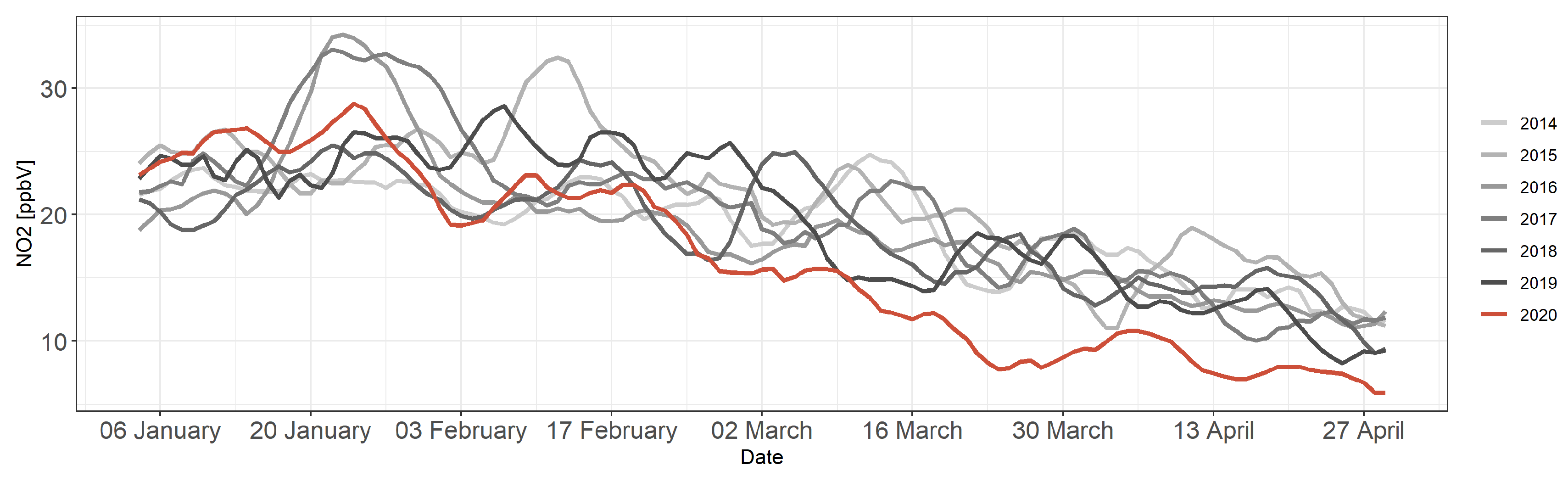
2.1. The “COVID” Case Study

In this study, the impact of COVID-19 containment measures on Lombardy’s air quality is quantified by comparing two simulations, which consider the emission reductions during the lockdown, with a reference BAU scenario. To highlight the importance of traffic reduction on NO2 concentration variations, the LOCK_TRA scenario assumes that only transport-related emissions are reduced, while the more realistic LOCK_ALL scenario also accounts for the decline in industrial activities. The application of increasingly rigorous and containment measures in Lombardy was made weekly, and for that reason, the two scenarios are designed by rescaling BAU emissions with weekly emission reduction factors. Figure 2 shows the timeline with the main government decrees and the setup of the three simulations. The case study is focused on a five-week period, from 24 February to the end of March, and LOCK_TRA and LOCK_ALL are the same until 23 March, when only factories attributable to essential supply chains were authorized to remain operative. The period before 24 February can be considered as a spin-up. More implementation details are provided in Section 2.3.
Comparing the measured concentration values at the ARPA (Agenzia Regionale per la Protezione dell’Ambiente) Lombardia sites with previous years shows the first sign of NO2 atmospheric concentration reduction during the lockdown. Figure 3 shows the NO2 concentration moving average from 2014 to 2020, for the first four months of each year.
The NO2 concentration contraction starts at the beginning of March, when the first containment measures were implemented, reaching halved values at the end of March, compared to previous years.
A statistical analysis on the averages was performed to assess if the difference in concentration observable in Figure 3 can be considered significant. Statistical software R [33] was used in combination with the R package rstatix [34]. The analysis focuses on two different periods:
  • Pre-lockdown: NO2 daily means from 1 January to 7 March for years 2014 to 2020;
  • Lockdown: NO2 daily means from 8 March to 30 April for years 2014 to 2020.
The Kruskal–Wallis rank sum test was used to check for a significant difference in daily averages among years, and the Mann–Whitney–Wilcoxon test with p-values adjusted with the Bonferroni method was used to identify where the difference occurs. A significant difference was found using Kruskal–Wallis for both periods, but the Mann–Whitney test found no difference between the year 2020 and every other year in the pre-lockdown period. A strong and significant difference was instead found in the lockdown period for the year 2020, with low adjusted p-values and a large effect size for the combination of the year 2020 and every other year. A summary of both test results can be found in Supplementary Material Tables S1–S3. The comparison of the statistical analysis results computed over the two different periods shows that the lockdown had a significant effect on NO2 concentration in the Lombardy region, causing a drop in the observed concentration.
Air pollutant concentration is affected by different factors, including weather, causing favorable or unfavorable conditions for pollutant diffusion, dispersion, and transformation. For this reason, an analysis of the main atmospheric circulation, during the case study period, was performed. This assessment was aimed at identifying the principal weather events of the period, on one hand, and to make a comparison with the weather of the previous years, which occurred in the same period, on the other.
During February and March 2020, the region was characterized by typical late winter/spring weather, with mostly sunny days, interrupted by a few days of rain. This period is also characterized by important changes in wind regimes, both in terms of direction and intensity. Figure 4 shows the air temperature, relative humidity, wind velocity, and total daily precipitation trends observed in Milan, during the three years, between mid-February and the end of March. This preliminary analysis excludes the occurrence of unusual weather regimes during the period of time between February and March 2020. Analyzing the temperature trend in Figure 4 shows how 2019 and 2020 are very similar throughout, while 2018 experienced colder days until early March.
During February and March 2020, the region was characterized by typical variability of late winter and spring weather conditions, with a dynamic sequence of anticyclonic and cyclonic conditions. The period was also characterized by important changes in wind regimes, both in terms of direction and intensity. In order to evaluate the presence or absence of particular meteorological conditions during the case study period, a brief analysis was carried out by comparing the time series of the surface variables affecting the lower atmosphere during recent years. Figure 4 shows the last three-year time series of air temperature, relative humidity, wind velocity, and total daily precipitation observed in Milan, between mid-February and the end of March. Analyzing the temperature in Figure 4, it can be noticed that in 2019 and 2020, this variable shows similar variability for both years, while 2018 experienced colder days until early March. Considering the wind intensity, comparable patterns can be noticed for 2019 and 2020, while 2018 shows, in general, lower wind intensities. Instead, 2018 appears more similar to 2020 in terms of precipitation, with many rainy days and significant rainfall. Considering relative humidity, important fluctuations characterize all the years. The years 2019 and 2020 differ from 2018 in their repeated cases of sudden drops in air humidity due to the presence of strong wind events.
A more detailed description of the meteorological conditions which occurred during the lockdown is reported. In Figure 5, the maps of the geopotential height Z (dam) and temperature at the 850 hPa level (a,c,e,g) in correspondence with the more interesting weather situations are also presented. To give an idea of the effect of the general circulation in the lower atmosphere, the corresponding planetary boundary layer (PBL) height is also reported alongside.
The beginning of February was characterized by the presence of strong winds and some weak perturbations with rain, resulting in favorable conditions for a pollutant concentration decrease. Later, an anticyclonic circulation occurred, resulting in a steady atmosphere and favorable conditions for pollutant accumulation. This period was interrupted by an intense foehn event, a warm and dry downslope wind descending the Alps as a result of cross-barrier flow over the mountain range. This is characterized by strong and gusty winds, hence favoring pollutant dispersion. The evidence of this phenomenon can be seen in Figure 5a, in the nose-like profile in the pressure ridge over the Alps, on the northern border of Lombardy. An important effect of this circulation was the presence of a very high PBL (Figure 5b), with favorable conditions for pollutant dispersion.
During the second half of the month, the weather changed often, with stable and warm weather, as represented, for example, in the geopotential map of Figure 5c related to the 15 of February, accompanied by low values of the PBL height (Figure 5d), interrupted by weak rain and another foehn event at the end of the month. The foehn brought intense winds and a drop in humidity, enhancing the effect of the initial measures adopted to face the COVID-19 epidemic, with a drastic reduction in pollutant concentrations.
The month of March was characterized by weather conditions typical of early spring, with variable weather, rainy at the beginning, followed by a significant increase in temperature and low wind during the week 16–22 March. These environmental conditions led to stable conditions of the atmosphere favorable for pollutant accumulation, and an example can be observed on 17 March when an anticyclonic ridge affected Central Europe (Figure 5e,f). Nevertheless NO2 concentration is reduced with respect to previous years (Figure 3).
A noteworthy meteorological event was the strong advection of dust, deriving from the Sahara, the Caspian Sea, and the Karakorum Desert, toward the Mediterranean basin at the end of March. This desert dust intrusion caused a huge concentration of particulate matter in the Lombardy region. In Figure 5g, related to 25 March, a deep low-pressure system over North Africa and the Mediterranean Sea generated intense easterly winds blowing toward the Po valley with a consequent transport of dust. Although this event did not affect the NO2 concentration, it is useful to point out the importance of meteorological analysis in air quality studies.

2.2. CAMx Configuration and Input Data

The Comprehensive Air Quality Model with Extensions (CAMx) model v6.30 [35] was used to calculate the concentration of NO2 throughout Italy, between mid-February and the end of March 2020. The model was applied over a computational domain covering all of the Italian peninsula with a spatial resolution of 4 km (Figure 1) and 14 terrain-following vertical levels. For this study, only the portion of the domain covering Lombardy is analyzed and shown. The overall configuration of the modeling chain follows the one presented in Meroni et al. [36] and Giani et al. [37], the main difference being the use of the traditional Secondary Organic Aerosol Processor (SOAP) [38] aerosol scheme for organic matter modeling. The meteorological input derives from a customized configuration of the numerical weather prediction (NWP) model Weather Regional Forecast (WRF) [39]. WRF is driven by initial and boundary conditions provided every 6 h by the Global Forecast System (GFS) produced by the European National Centers for Environmental Prediction (NCEP). WRF-ARW (version 3.9) was used to perform the dynamical downscaling of the GFS. The WRF model is managed by the University Corporation for Atmospheric Research (UCAR), which is a consortium of about a hundred American universities. UCAR provides a major-release update at least once a year. The current set of parameterizations was chosen after many sensitivity tests. The computational domain and the spatial resolution of the WRF model are the same as those used for CAMx except for a frame of buffer cells at the edge of the grid, added to avoid boundary effects. The convection was explicit and the vertical levels of the models were set to 36. Finally, a spectral nudging technique [40,41] was also performed to better drive the large-scale fields within the WRF-ARW domain, allowing a better coherency with the GFS forecast. Spectral nudging was applied on the geopotential field, temperature, and horizontal wind components at all vertical model levels. Additionally, temperature and horizontal wind components were nudged within the PBL. After some sensitivity tests on NO2 concentration with different emission inventories, i.e., the European Monitoring and Evaluation Program (EMEP) gridded emission inventory and the Italian national inventory of anthropogenic emissions developed by ISPRA (Istituto Superiore per la Protezione e la Ricerca Ambientale), the latter was used for the Italian fraction of the domain, while EMEP (2010 version) was used outside Italy. In particular, we used the latest version available of the inventory, i.e., ISPRA 2015, even though a decreasing trend in Italian NOx emissions was reported in the National Inventory Report [42] with specific reference to the years from 1990 to 2016. In particular, the emissions of NOx into the atmosphere related to the road transport sector are gradually decreasing [43].
Both the inventories were processed with the Sparse Matrix Operator for Kernel Emission model (SMOKE v3.5) [44] in order to obtain hourly gridded emission fields over the domain. Then, biogenic and sea salt emissions estimated, respectively, using the Model of Emissions of Gases and Aerosols from Nature (MEGAN v2.03) [45] and the SEASALT model [46,47] were added to the anthropogenic emissions. Boundary and initial conditions necessary for CAMx were obtained from the CHIMERE model using INERIS’ Prev’Air service [48].

2.3. Emission Scenarios

The case study analyzed in this work starts on 10 February and is composed of a spin-up period of two weeks (during which BAU and scenarios correspond) and then a five-week simulation, each one taking into account the restrictions imposed by the COVID-19 containment measures, according to the methodological scheme shown in Figure 2. The estimate of regional emissions during the lockdown was published by ARPA Lombardia [49], which provides specific reduction rates for the main emission sources. These rates are estimated by assessing the variation in environmental pressure factors, based on different data sources. Road traffic was calculated by means of data collected for the Move-In (MOnitoraggio dei VEicoli INquinanti) project [50], which is a regional service for emission monitoring. Other data from highways and roads were provided by ANAS [51] (Azienda Nazionale Autonoma delle Strade), who is in charge of the maintenance of Italian roads. More precisely, the variation in traffic flows on urban and extra-urban roads and highways for cars, light-duty vehicles, and heavy-duty vehicles was evaluated for the months of the lockdown. Flight data from Eurocontrol and radar tracks (collected by ARPA Lombardia) were considered to evaluate the decrease in emissions from planes and airports’ activities. The variation in industrial activities and domestic heating was estimated from data of the electric energy load published by TERNA [52] and of natural gas consumption published by SNAM [53]. Furthermore, data from regional emission monitoring networks and agriculture activities were included in the evaluation. By the knowledge of the emission factors for each activity available in INEMAR [54], the regional emission inventory database, and the variations in activities, the change in emissions of the principal pollutants was calculated on a daily basis. Albeit the reduction in industrial activities has relevant effects, such coefficients suggest that road traffic is the main element responsible for the drastic reduction in NOX emissions. The LOCK_ALL scenario, including also such effects, allows highlighting the share of air quality improvement due to the reduction in combustion in the manufacturing industry (SNAP 03) as well as production processes (SANP 04) with respect to traffic. For what concerns road transport emissions (SNAP 07), different coefficients were used for the metropolitan area of Milan, where we were able to distinguish private transport from public and commercial, which is less affected by COVID-19 containment measures. In the city of Milan, traffic reduction coefficients are calculated and published by the city’s mobility and environment agency, AMAT. During the lockdown, hourly traffic counts collected by the automatic control systems of both “Area B” (a Low Emission Zone that includes most parts of the city, i.e., 72% of the municipality and 98% of the population) and “Area C” (the Congestion Charge Area of the city center) were published [55]. The two datasets, which have different characteristics, were merged in order to quantify the distinction between private/public vehicles and passenger/commercial vehicles.
Under the assumption of linearity between road traffic intensity and atmospheric emissions, the aforementioned coefficients were applied to all pollutants simulated by the CAMx model. To this aim, the SMOKE model was used to simulate the emission scenario fields by applying reduction coefficients to the BAU scenario emission fields. All the reduction coefficients used in this work, for both the Lombardy region and the metropolitan area of Milan, are summarized in Table 1 and Table 2, respectively.

3. Results

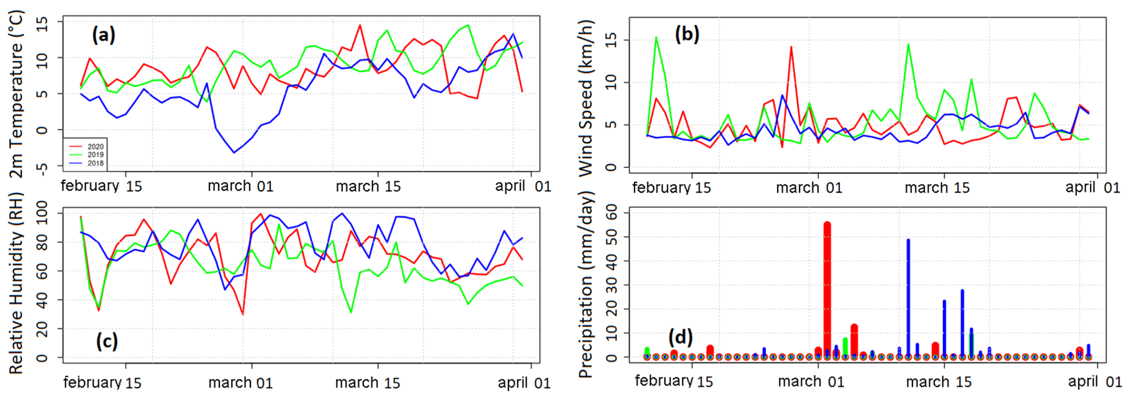
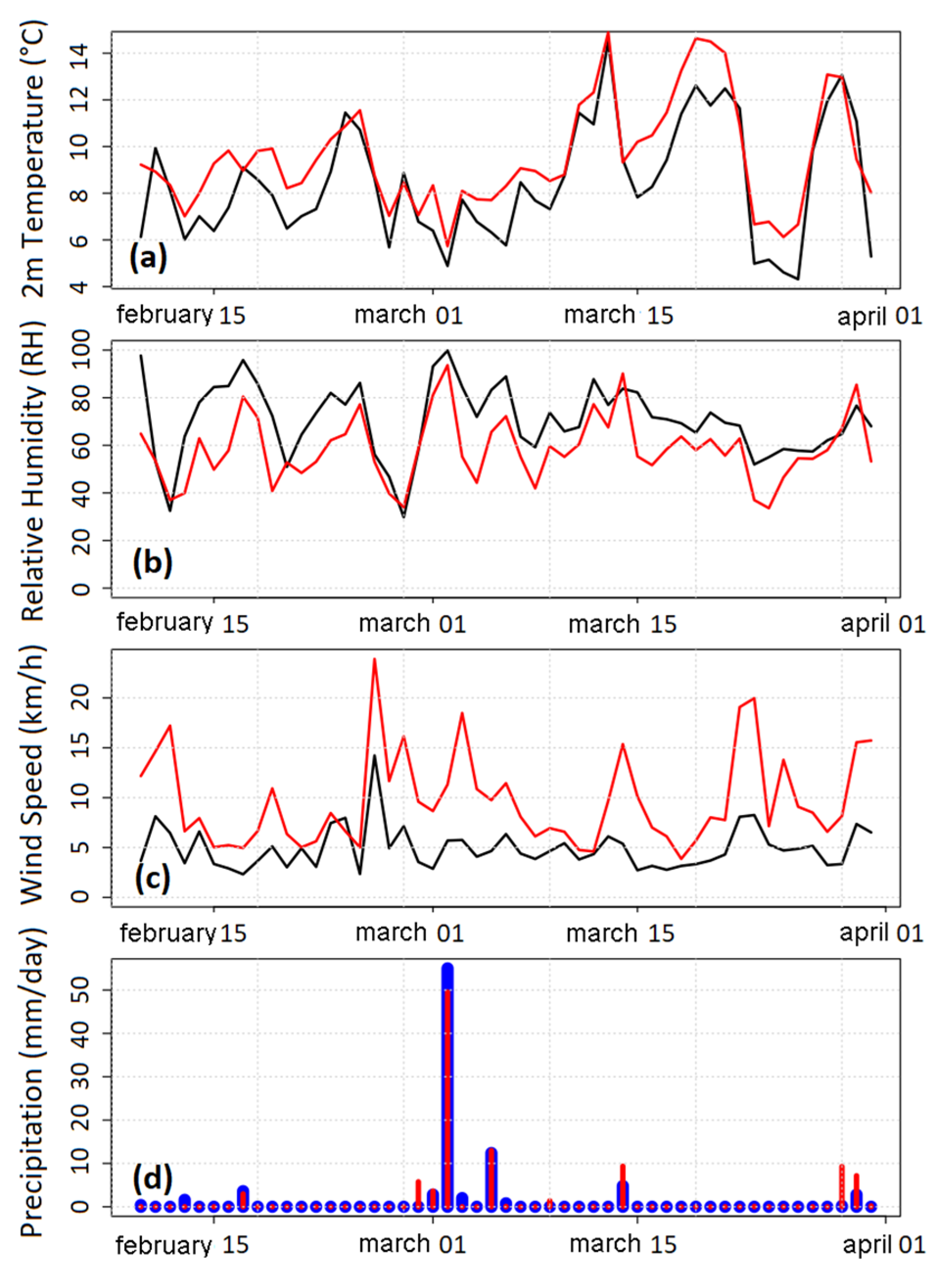
3.1. Meteorological Parameters

This work provides an overall understanding of how the physical and chemical dynamics have characterized the first part of the spring lockdown in Lombardy. We aim to analyze how meteorological processes have allowed or prevented the improvement in air quality due to emissions reduction. Figure 6 shows the validation of the simulated meteorological parameters with the observations. The measured air temperature trend, relative humidity, wind intensity, and rainfall recorded in the city of Milan are compared to the modeled variables. In general, a good agreement between observations and modeled variables is found, except for the wind speed where a partial overestimation for the city of Milan can be observed. Such behavior can be partially attributed to the resolution of the model, which is too coarse to represent properly the friction caused by the presence of the urban canopy fabric and consequently the wind speed reduction.

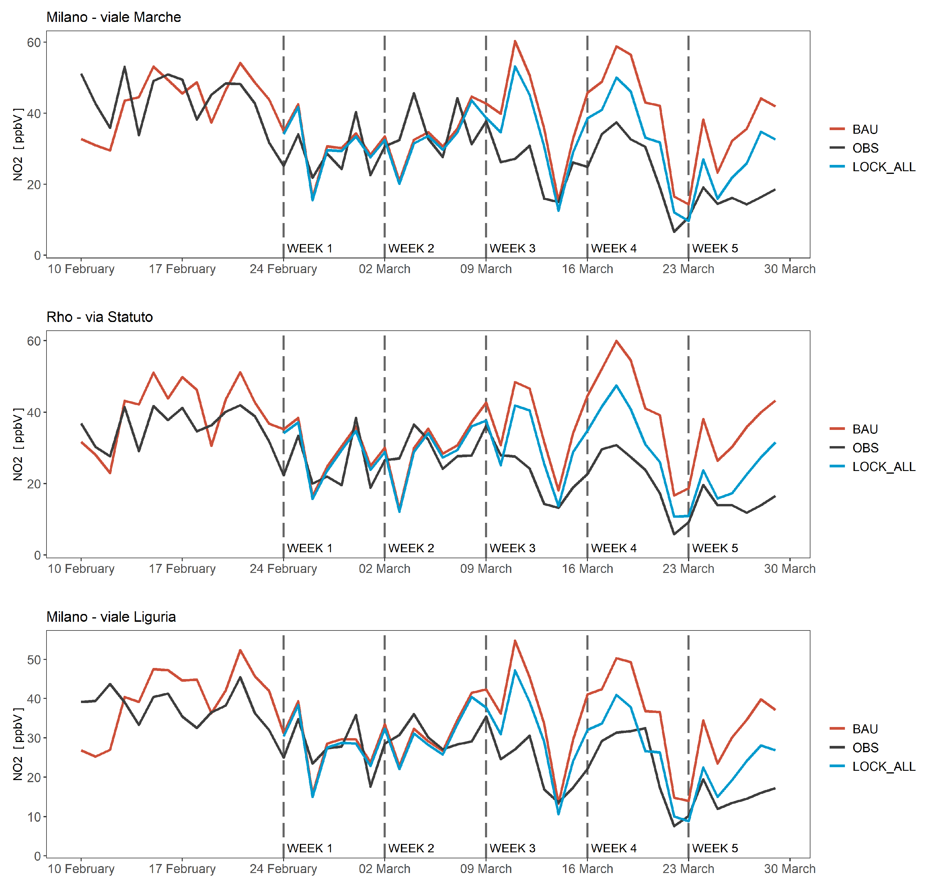
3.2. NO2 Concentration

Lombardy is characterized by inhomogeneous orographic and demographic characteristics as well as by a high gradient of NO2 atmospheric concentration distribution. The highest values are reached in the city of Milan and its surroundings. The CAMx model, with 4 km of horizontal resolution, can simulate properly the NO2 concentration gradient. In Figure 7a,c, the average BAU weekly concentration of NO2 is shown, respectively, for the first and the last weeks of March 2020, corresponding to the second and fifth week of the analyzed period. Besides the capital city of Milan, where the average nitrogen dioxide concentration exceeds 30 ppbV during March, another highly polluted area is the province of Monza e Brianza as well as the fraction of Bergamo, Como, and Varese provinces which is placed in the Po Valley. Another spot, characterized by high NO2 concentration, is located around the city of Brescia. The air quality benefit caused by the lockdown can be appreciated in Figure 7b,d, where the absolute difference between the LOCK_ALL scenario and BAU is shown, for the previously mentioned two weeks. As expected, the most important reductions are found in the Metropolitan City of Milan and neighboring areas, along with the highways A1, A4, and A14, albeit in a more contained way. During the first week of March (from 2 to 8 March), due to the small slowdown of human activities, the lockdown caused a reduction in NO2 concentration that rarely exceeded 1 ppbV, with an average value of −0.4 ppbV and a maximum of −1.2 ppbV. After three weeks, the CAMx model estimated a reduction of about −12 ppbV in Milan and about −5 ppbV in the remaining highly polluted part of the region. The impact of the industrial sector is estimated by comparing the two LOCK_ALL and LOCK_TRA scenarios. The shutdown of non-essential industrial activities put in place by the government at the beginning of week 4 led to a further drop in concentration, but with low values compared to the reduction in concentration caused by the road transport sector. The share of the overall difference in concentration levels between the BAU scenario and LOCK_ALL averaged over Lombardy due to the industrial sector (SNAP 3 and 4) is 7.2% in week 4 and 9.4% in week 5. As shown in Figure 8, the difference in concentration between the two scenarios is appreciable only in the provinces of Bergamo, Brescia, and Varese, where the values are higher than the average, with a concentration drop of around 15−20%. Other results for weeks 2, 3, and 4 can be found in the Supplementary Materials.
Moreover, comparing the NO2 hourly mean concentration simulated with CAMx (BAU, LOCK_TRA and LOCK_ALL) with air quality data from the ARPA Lombardia database [56] allows for the following:
  • Calculating the difference between the BAU and lockdown scenarios, day by day, during all of the case study period;
  • Estimating the impact of meteorological conditions on NO2 atmospheric concentration;
  • Understanding what is the impact of reduced mobility with respect to the overall decrease in human activity;
  • Performing sensitivity tests and calibrating CAMx simulations;
  • Assessing the methodology implemented to calculate NO2 emissions during the lockdown.
The validation for the six stations listed in Table 3 and shown in Figure 1 is discussed below, while the exact position of each monitoring station with respect to the urban structure can be found in the Supplementary Material Figure S1.
Figure 9 and Figure 10 show NO2 time series measured and simulated with CAMx model, respectively for the city of Milan and for the cities of Bergamo and Brescia, during the case study period. As introduced in Section 2.1, during the analyzed period, unstable and stable atmospheric conditions succeeded one another, leading to, respectively, dispersion and accumulation of the NO2 atmospheric concentration. The role of primary nitrogen dioxide [57] emissions in the development of NO2 concentrations in a traffic environment explains the immediate response of the NO2 atmospheric concentration once the measures adopted to face the COVID-19 pandemic started. This trend can be appreciated in both the modeled and measured time series. The reduction in pollutant concentration was enhanced by the foehn event at the end of February. Another example of the impact of meteorological conditions on NO2 concentration is the increase in temperature and low wind during the week 16–22 March. These factors led to stable conditions of the atmosphere, then the accumulation of NO2 concentration. For the six selected sites, the agreement between BAU-simulated NO2 values and the observations during the pre-pandemic period is quite good as well as for the first two weeks of the analyzed period. The lockdown scenarios start to diverge from BAU after 9 March, once stronger containment measures were applied and most of the population stayed home, and the reduction coefficients concerning road traffic are three times larger with respect to the previous week. As expected from this moment, both LOCK_ALL- and LOCK_TRA-simulated concentrations approach the observed values. Nevertheless, during the third and fourth weeks, the CAMx model tends to overestimate NO2 concentration and this mismatch can be due to several causes. First of all, local sources can affect measured concentrations that a 4 km resolution chemical transport model cannot reproduce well. Figure S1 shows the geographical location of all monitoring stations analyzed in this work with respect to the CAMx computational grid. Depending on the urban structure contained in the grid cell, the modeled concentration can be more or less representative of the measured one at a monitoring site. Further, modeling assumptions can be at the origin of this mismatch, e.g., using a five years earlier inventory which tends to overestimate human activities and related emissions [42,43]. Finally, for the fifth week, the modeled LOCK_ALL scenario NO2 values match very well with the observations, especially for Treviglio and Bergamo via Garibaldi sites.

4. Discussion

The lockdown imposed on the Lombardy region and then extended to the whole country has allowed, for the first time, researchers to assess and quantify what is the impact of the huge reduction in road traffic emissions on air quality. Moreover, the more and more incisive lockdown measures allowed us to evaluate the impact on pollutant concentration of gradual emission reductions, providing realistic indications on the traffic limitation that should be imposed to reach specific air quality targets. As expected, road transport has a relevant effect on the atmospheric concentration of NO2. The CAMx model estimates that if road traffic reduces by 12%, the NO2 atmospheric concentration reduces by about −4%, while for a reduction of one third of the NO2 concentration, road traffic should be reduced by about 70%. The exact weekly average correspondence between emissions and NO2 concentration reduction is found in Table 2 and Table 3, respectively, for Lombardy and the city of Milan. Road transport yields, on a yearly basis, about 50% and 65% of NOX emissions over Lombardy and Milan, respectively [49]. During winter, such relative contribution is slightly lower due to the residential heating. Therefore, a reduction of 77% in the NOX emissions of road transport implies about a 30–35% reduction in total NOX emissions over Lombardy, roughly corresponding to a relative reduction in NO2 concentration. Similar results can be obtained for other emission reduction levels, as can be inferred from Table 2 and Table 3. This result provides a rather clear relationship between NOX emission reduction for road transport and NO2 concentration decline, thus providing valuable support for policy-makers. The lockdown also offers a unique chance to assess the modeling chain performances in simulating sustainable mobility-like scenarios as well as the methodology to build the scenario (discussed in Section 2.3). Even if it is well known that road transport is the greatest source of NOX emissions and therefore the main factor responsible for the NO2 concentration [58], the more realistic scenario LOCK_ALL was built, in order to match, as much as possible, the observations. After all, a good agreement between LOCK_ALL and measured NO2 concentration was found, confirming the reliability of the implemented approach. The results of this study are comparable with other works published in the literature and mentioned in Section 1. The report published in the frame of the European life project PREPAIR [27] estimates a reduction of 35–50% in NO2 atmospheric concentration for the Po Valley region, during the second half of March. Another study published by SNPA (Sistema Nazionale Protezione Ambiente) estimates that nitrogen dioxide has reduced by 40% over Lombardy [30]. Moreover, Menut et al. [31] found a maximum daily concentration delta reached in March of about 44% in both urban and rural areas, using a modeling approach. The results found for Lombardy are more incisive for the city of Milan, which normally attracts more than 350,000 workers and 100,000 students every day [59] and which has the role of being the cultural and economic hub of the region. According to the city of Milan statistical analysis published in 2011, most commuters going to the capital city as well as 36% of its residents prefer private transport compared to public [59]. Consequently, the air quality improvement in the city of Milan during the lockdown can be attributed exclusively to the reduction in road traffic, e.g., during the last week of March, the NO2 concentration decreased by about 10 ppbV, which is twice the value reached in Bergamo and Brescia.

5. Conclusions

The first COVID-19 containment measures in Europe were enforced on Italy, initially in Lombardy, on 24 February, when schools closed. Travel restrictions and the obligation for people to remain at homes were imposed two weeks after and, at the end of March, all unnecessary commercial and production activities stopped. The study is focused on nitrogen dioxide (NO2), a pollutant that is harmful to human health and strongly correlated with vehicular traffic, therefore particularly suitable for a study on the impact of mobility on air quality. A quantitative assessment of the effects of the lockdown was carried out, by comparing three simulations, one with standard emissions (BAU) and the other two with reduced emissions, in road traffic (LOCK_TRA) and all affected emission sources (LOCK_ALL). Obtained results show that NOX emission reduction, over the whole region, ranges between 12% and 74% with corresponding reductions in NO2 concentrations ranging between 4.3% and 33.7%, which corresponds to a decrease of about 20 ppbV in the areas of maximum pollution. Similar results are obtained in the city of Milan. Modeled NO2 concentrations for BAU, LOCK_TRA, and LOCK_ALL were then compared with the measured values at six sites, showing a good agreement with observations in both pre- and post-pandemic periods. For the first time, we are able to validate the modeling chain’s ability to reconstruct reduced mobility, emissions, and pollutant concentration. The validation of the weather forecasting used in the input to CAMx, strengthens the quality of the results obtained from the modeling suite, allowing for demarcating the effects of emission reduction on pollutant concentration concerning meteorological conditions.
Besides the analysis of a specific case study about the effects of the spring lockdown on air quality, more general consideration can be taken of the effectiveness of mobility policies to achieve environmental targets. Regarding NO2, a real improvement in air quality is achieved after significant reductions in road emissions (over 70%). For this reason, incisive and realistic mobility policies should include a wide spectrum of intervention areas. Wide-ranging strategies, based on a substantial reduction in mobility as a whole, are needed. Smart working could help mobility management as well as redesigning urban areas to ensure proximity services for citizens and avoid unnecessary driving. Along with these facility changes, it is necessary to promote a “modal shift” towards more sustainable modes of transport, e.g., increasing walking and cycling, car sharing, and the use of public transport. In such a context, a greater benefit would derive from the renewal of a minimum indispensable vehicle fleet, replacing the cars currently in circulation with electric or low emission vehicles.

Supplementary Materials

The following are available online at https://0-www-mdpi-com.brum.beds.ac.uk/2073-4433/11/12/1319/s1, Figure S1: Location of air quality stations used in model validation with superimposed computational grid. (a) Bergamo—Via Garibaldi, (b) Treviglio, (c) Brescia—Broletto, (d) Milano—Viale Marche/Viale Liguria, (e) Rho—Via Statuto. Figure S2: NO2 weekly mean concentration (ppbV) for the BAU scenario for weeks 1 (a), 3 (c), and 4 (e). Absolute difference between LOCK_TRA and BAU scenarios for weeks 1 (b), 3 (d), and 4 (f). Figure S3: Computational domain of WRF-ARW with the underlying orography. The grid has a horizontal resolution of 4 km, and the simulations were conducted with 36 vertical levels. Table S1: Kruskal–Wallis test summary for pre-lockdown and lockdown period. Table S2: Mann–Whitney–Wilcoxon test summary report for pre-lockdown period. Table S3: Mann–Whitney–Wilcoxon test summary report for pre-lockdown period.

Author Contributions

Conceptualization: A.P., V.A. and G.P.; methodology: A.P., V.A., A.B. and G.P.; validation: R.B. and M.L.; formal analysis: A.P., V.A., A.B., M.B. and F.R.; investigation: E.C., R.B. and M.L.; writing—original draft: A.P., V.A., G.P., G.L., M.B., E.C., R.B. and M.L.; writing—review and editing: V.A, A.B., M.B., R.B., E.C., F.C., M.L., G.L., A.P., G.P., F.R., G.M.R, A.M.T.; visualization: A.P. and R.B.; supervision: A.B., G.P. and G.M.R. All authors have read and agreed to the published version of the manuscript.

Funding

This work has been financed by Research Fund for the Italian Electrical System with the Decree of 16 April 2018.

Acknowledgments

We thank the reviewers for their comments on the manuscript.

Conflicts of Interest

The authors declare no conflict of interest. The funders had no role in the design of the study; in the collection, analyses, or interpretation of data; in the writing of the manuscript, or in the decision to publish the results.

References

  1. Fenger, J. Urban air quality. Atmos. Environ. 1999, 33, 4877–4900. [Google Scholar] [CrossRef]
  2. World Health Organization. Health Effects of Transport-Related Air Pollution; Krzyżanowski, M., Kuna-Dibbert, B., Schneider, J., Eds.; World Health Organization: Geneva, Switzerland, 2005. [Google Scholar]
  3. Hitchcock, G.; Conlan, B.; Kay, D.; Brannigan, C.; Newman, D. Air Quality and Road Transport Impacts and Solutions; RAC Foundation: London, UK, 2014. [Google Scholar]
  4. European Economic Area. Transport and Public Health. Available online: https://www.eea.europa.eu/downloads/b396ad0066184a778099dbf50a0c88d9/1606129104/transport-and-public-health.pdf (accessed on 25 November 2020).
  5. Tsakalidis, A.; van Balen, M.; Gkoumas, K.; Pekar, F. Catalyzing sustainable transport innovation through policy support and monitoring: The case of TRIMIS and the European green deal. Sustainability 2020, 12, 3171. [Google Scholar] [CrossRef] [Green Version]
  6. Bao, R.; Zhang, A. Does lockdown reduce air pollution? Evidence from 44 cities in northern China. Sci. Total Environ. 2020, 731, 139052. [Google Scholar] [CrossRef]
  7. Cole, M.A.; Elliott, R.J.R.; Liu, B. The Impact of the Wuhan Covid-19 Lockdown on Air Pollution and Health: A Machine Learning and Augmented Synthetic Control Approach. Environ. Resour. Econ. 2020, 76, 553–580. [Google Scholar] [CrossRef]
  8. Brimblecombe, P.; Lai, Y. Effect of sub-urban scale lockdown on air pollution in Beijing. Urban Clim. 2020, 34, 100725. [Google Scholar] [CrossRef]
  9. Silver, B.; He, X.; Arnold, S.R.; Spracklen, D.V. The impact of COVID-19 control measures on air quality in China. Environ. Res. Lett. 2020, 15, 084021. [Google Scholar] [CrossRef]
  10. Singh, R.P.; Chauhan, A. Impact of lockdown on air quality in India during COVID-19 pandemic. Air Qual. Atmos. Health 2020, 13, 921–928. [Google Scholar] [CrossRef]
  11. Berman, J.D.; Ebisu, K. Changes in U.S. air pollution during the COVID-19 pandemic. Sci. Total Environ. 2020, 739, 139864. [Google Scholar] [CrossRef]
  12. Sicard, P.; De Marco, A.; Agathokleous, E.; Feng, Z.; Xu, X.; Paoletti, E.; Rodriguez, J.J.D.; Calatayud, V. Amplified ozone pollution in cities during the COVID-19 lockdown. Sci. Total Environ. 2020, 735, 139542. [Google Scholar] [CrossRef]
  13. Zangari, S.; Hill, D.T.; Charette, A.T.; Mirowsky, J.E. Air quality changes in New York City during the COVID-19 pandemic. Sci. Total Environ. 2020, 742, 140496. [Google Scholar] [CrossRef]
  14. Jia, C.; Fu, X.; Bartelli, D.; Smith, L. Insignificant Impact of the “Stay-At-Home” Order on Ambient Air Quality in the Memphis Metropolitan Area, USA. Atmosphere 2020, 11, 630. [Google Scholar] [CrossRef]
  15. President of the Council of Ministers of the Italian Republic Decree of the President of the Council of Ministers of the Italian Republic of 1 March 2020—Further Implementing Provisions of the Decree-Law of 23 February 2020, n. 6, Containing Urgent Measures Regarding the Containment and Management of the Epidemiol. Available online: https://www.gazzettaufficiale.it/eli/id/2020/03/01/20A01381/sg (accessed on 25 November 2020).
  16. President of the Council of Ministers of the Italian Republic Decree of the President of the Council of Ministers of the Italian Republic of 8 March 2020—Further Implementing Provisions of the Decree-Law of 23 February 2020, n. 6, Containing Urgent Measures Regarding the Containment and Management of the Epidemiological Emergency from COVID-19. Available online: https://www.gazzettaufficiale.it/eli/id/2020/03/08/20A01522/sg (accessed on 25 November 2020). (In Italian).
  17. President of the Council of Ministers of the Italian Republic Decree of the President of the Council of Ministers of the Italian Republic of 11 March 2020—Further Implementing Provisions of the Decree-Law of 23 February 2020, n. 6, Containing Urgent Measures Regarding the Containment and Management of the Epidemiological Emergency from COVID-19. Available online: https://www.gazzettaufficiale.it/eli/id/2020/03/11/20A01605/sg (accessed on 25 November 2020). (In Italian).
  18. President of the Council of Ministers of the Italian Republic Decree of the President of the Council of Ministers of the Italian Republic of 22 March 2020—Further Implementing Provisions of the Decree-Law of 23 February 2020, n. 6, Containing Urgent Measures Regarding the Containment and Management of the Epidemiological Emergency from COVID-19. Available online: https://www.gazzettaufficiale.it/eli/id/2020/03/22/20A01807/sg (accessed on 25 November 2020). (In Italian).
  19. Collivignarelli, M.C.; Abbà, A.; Bertanza, G.; Pedrazzani, R.; Ricciardi, P.; Carnevale Miino, M. Lockdown for CoViD-2019 in Milan: What are the effects on air quality? Sci. Total Environ. 2020, 732, 1–9. [Google Scholar] [CrossRef]
  20. Carugno, M.; Consonni, D.; Bertazzi, P.A.; Biggeri, A.; Baccini, M. Temporal trends of PM10 and its impact on mortality in Lombardy, Italy. Environ. Pollut. 2017, 227, 280–286. [Google Scholar] [CrossRef]
  21. Van Donkelaar, A.; Martin, R.V.; Brauer, M.; Boys, B.L. Use of Satellite Observations for Long-Term Exposure Assessment of Global Concentrations of Fine Particulate Matter. Environ. Health Perspect. 2015, 123, 135–143. [Google Scholar] [CrossRef] [Green Version]
  22. Caserini, S.; Giani, P.; Cacciamani, C.; Ozgen, S.; Lonati, G. Influence of climate change on the frequency of daytime temperature inversions and stagnation events in the Po Valley: Historical trend and future projections. Atmos. Res. 2017, 184, 15–23. [Google Scholar] [CrossRef] [Green Version]
  23. Pernigotti, D.; Georgieva, E.; Thunis, P.; Cuvelier, C.; de Meij, A. The Impact of Meteorology on Air Quality Simulations over the Po Valley in Northern Italy; Springer: Dordrecht, The Netherlands, 2011; pp. 485–490. [Google Scholar]
  24. Perrino, C.; Catrambone, M.; Dalla Torre, S.; Rantica, E.; Sargolini, T.; Canepari, S. Seasonal variations in the chemical composition of particulate matter: A case study in the Po Valley. Part I: Macro-components and mass closure. Environ. Sci. Pollut. Res. 2014, 21, 3999–4009. [Google Scholar] [CrossRef]
  25. Larsen, B.R.; Gilardoni, S.; Stenström, K.; Niedzialek, J.; Jimenez, J.; Belis, C.A. Sources for PM air pollution in the Po Plain, Italy: II. Probabilistic uncertainty characterization and sensitivity analysis of secondary and primary sources. Atmos. Environ. 2012, 50, 203–213. [Google Scholar] [CrossRef]
  26. Kukkonen, J.; Pohjola, M.; Sokhi, R.S.; Luhana, L.; Kitwiroon, N.; Fragkou, L.; Rantamäki, M.; Berge, E.; Ødegaard, V.; Slørdal, L.H.; et al. Analysis and evaluation of selected local-scale PM10 air pollution episodes in four European cities: Helsinki, London, Milan and Oslo. Atmos. Environ. 2005, 39, 2759–2773. [Google Scholar] [CrossRef]
  27. Deserti, M.; Raffaelli, K.; Ramponi, L.; Carbonara, C. Studio Preliminare Degli Effetti Delle Misure COVID-19 Sulle Emissioni in Atmosfera E Sulla Qualità Dell’aria nel Bacino Padano; ARPAE Emilia-Romagna: Emilia-Romagna, Italy, 2020. [Google Scholar]
  28. Cameletti, M. The Effect of Corona Virus Lockdown on Air Pollution: Evidence from the City of Brescia in Lombardia Region (Italy). Atmos. Environ. 2020, 239, 117794. [Google Scholar] [CrossRef]
  29. Rossi, R.; Ceccato, R.; Gastaldi, M. Effect of Road Traffic on Air Pollution. Experimental Evidence from COVID-19 Lockdown. Sustainability 2020, 12, 8984. [Google Scholar] [CrossRef]
  30. SNPA Pianura Padana, Graduale Riduzione Della Concentrazione di Biossido di Azoto (NO2) Nelle Ultime Settimane—SNPA—Sistema Nazionale Protezione Ambiente. Available online: https://www.snpambiente.it/2020/03/23/pianura-padana-biossido-di-azoto-no2-graduale-riduzione-della-concentrazione-nelle-ultime-settimane/ (accessed on 24 September 2020).
  31. Menut, L.; Bessagnet, B.; Siour, G.; Mailler, S.; Pennel, R.; Cholakian, A. Impact of lockdown measures to combat Covid-19 on air quality over western Europe. Sci. Total Environ. 2020, 741, 140426. [Google Scholar] [CrossRef]
  32. Guevara, M.; Jorba, O.; Soret, A.; Petetin, H.; Bowdalo, D.; Serradell, K.; Tena, C.; Denier van der Gon, H.; Kuenen, J.; Peuch, V.-H.; et al. Time-resolved emission reductions for atmospheric chemistry modelling in Europe during the COVID-19 lockdowns. Atmos. Chem. Phys. 2020, 1–37. [Google Scholar] [CrossRef]
  33. R Core Team R. A Language and Environment for Statistical Computing; R Foundation for Statistical Computing: Vienna, Austria, 2019. [Google Scholar]
  34. Kassambara, A. Rstatix: Pipe-Friendly Framework for Basic Statistical Tests. 2020. Available online: https://github.com/kassambara/rstatix (accessed on 5 December 2020).
  35. Environ CAMx User Guide v6.3; Ramboll Environ: Novato, CA, USA, 2016; 273p.
  36. Meroni, A.; Pirovano, G.; Gilardoni, S.; Lonati, G.; Colombi, C.; Gianelle, V.; Paglione, M.; Poluzzi, V.; Riva, G.M.; Toppetti, A. Investigating the role of chemical and physical processes on organic aerosol modelling with CAMx in the Po Valley during a winter episode. Atmos. Environ. 2017, 171, 126–142. [Google Scholar] [CrossRef]
  37. Giani, P.; Balzarini, A.; Pirovano, G.; Gilardoni, S.; Paglione, M.; Colombi, C.; Gianelle, V.L.; Belis, C.A.; Poluzzi, V.; Lonati, G. Influence of semi- and intermediate-volatile organic compounds (S/IVOC) parameterizations, volatility distributions and aging schemes on organic aerosol modelling in winter conditions. Atmos. Environ. 2019, 213, 11–24. [Google Scholar] [CrossRef] [Green Version]
  38. Strader, R.; Lurmann, F.; Pandis, S.N. Evaluation of secondary organic aerosol formation in winter. Atmos. Environ. 1999, 33, 4849–4863. [Google Scholar] [CrossRef]
  39. Skamarock, W.C.; Klemp, J.B.; Dudhia, J. A Description of the Advanced Research WRF Version 3. Tech. Note NCAR/TN-475+STR 2008. [Google Scholar] [CrossRef]
  40. Von Storch, H.; Langenberg, H.; Feser, F. A spectral nudging technique for dynamical downscaling purposes. Mon. Weather Rev. 2000, 128, 3664–3673. [Google Scholar] [CrossRef]
  41. Liu, P.; Tsimpidi, A.P.; Hu, Y.; Stone, B.; Russell, A.G.; Nenes, A. Differences between downscaling with spectral and grid nudging using WRF. Atmos. Chem. Phys. 2012, 12, 3601–3610. [Google Scholar] [CrossRef] [Green Version]
  42. Istituto Superiore per la Protezione e la Ricerca Ambientale. Italian Emission Inventory 1990–2018; Informative Inventory Report 2020; ISPRA: Roma, Italy, 2020; ISBN 978-88-448-0994-2.
  43. Iarocci, G.; Cocchiara, R.A.; Sestili, C.; Del Cimmuto, A.; La Torre, G. Variation of atmospheric emissions within the road transport sector in Italy between 1990 and 2016. Sci. Total Environ. 2019, 692, 1276–1281. [Google Scholar] [CrossRef]
  44. UNC SMOKE v3.5 User’s Manual. Available online: http://www.smoke-model.org/index.cfm (accessed on 3 December 2020).
  45. Guenther, A.; Karl, T.; Harley, P.; Wiedinmyer, C.; Palmer, P.I.; Geron, C. Estimates of global terrestrial isoprene emissions using MEGAN (Model of Emissions of Gases and Aerosols from Nature). Atmos. Chem. Phys. 2006, 6, 3181–3210. [Google Scholar] [CrossRef] [Green Version]
  46. Environ, R. Seasalt Guide Version 3.2; Seasalt Cornwall: Falmouth, UK, 2015. [Google Scholar]
  47. Gong, S.L. A parameterization of sea-salt aerosol source function for sub- and super-micron particles. Glob. Biogeochem. Cycles 2003, 17. [Google Scholar] [CrossRef]
  48. Institut National de l’EnviRonnement Industriel et des RisqueS (INERIS) PREV’AIR. Available online: http://www2.prevair.org/ (accessed on 24 September 2020).
  49. Marongiu, A.; Angelino, E.; Fossati, G.; Moretti, M.; Peroni, E.; Pantaleo, A.; Malvestiti, G.; Abbattista, M. Stima Preliminare Delle Emissioni in Lombardia Durante L’emergenza COVID-19; ARPA Lombardia—Agenzia Regionale per la Protezione dell’Ambiente della Lombardia: Milano, Italy, 2020.
  50. Move-In Regione Lombardia. Available online: https://www.movein.regione.lombardia.it/movein/#/index (accessed on 9 October 2020).
  51. Osservatorio del Traffico|Anas S.p.a. Available online: https://www.stradeanas.it/it/le-strade/osservatorio-del-traffico (accessed on 9 October 2020).
  52. Total Load—Terna S.p.a. Available online: https://www.terna.it/it/sistema-elettrico/transparency-report/total-load (accessed on 9 October 2020).
  53. SNAM. Available online: https://www.snam.it/it/trasporto/dati-operativi-business/2_Andamento_dal_2005/ (accessed on 9 October 2020).
  54. Inemar (Inemar. HomeLombardia). Available online: https://www.inemar.eu/xwiki/bin/view/Inemar/HomeLombardia (accessed on 9 October 2020).
  55. AMAT. Monitoraggio sistemi di mobilità durante l’emergenza Coronavirus—Agenzia Mobilità Ambiente Territorio. Available online: https://www.amat-mi.it/it/progetti/monitoraggio-mobilita-coronavirus/ (accessed on 24 September 2020).
  56. ARPA Lombardia Dati Sensori Aria|Open Data Regione Lombardia. Available online: https://www.dati.lombardia.it/Ambiente/Dati-sensori-aria/nicp-bhqi (accessed on 24 September 2020).
  57. Anttila, P.; Tuovinen, J.P.; Niemi, J.V. Primary NO2 emissions and their role in the development of NO2 concentrations in a traffic environment. Atmos. Environ. 2011, 45, 986–992. [Google Scholar] [CrossRef]
  58. European Environment Agency. Air Quality in Europe 2018; European Environment Agency: Copenhagen, Denmark, 2018. [Google Scholar]
  59. Settore Statistica Comune di Milano. Analisi del pendolarismo per studio e per lavoro a Milano; Settore Statistica Comune di Milano: Milano, Italia, 2020.
Figure 1. The Italian domain of simulation (a) and the Lombardy region domain of study (b) with its 13 provinces. The six markers show the position of the air quality stations analysed in this work.
Atmosphere 11 01319 g001
Figure 2. Correlation between the COVID-19 containment measures applied in the Lombardy region and the three simulations of this study.
Atmosphere 11 01319 g002
Figure 3. The 7-day moving average of NO2 atmospheric hourly concentration measured at ARPA Lombardia sites, from 1 January to 30 April for the years 2014–2020.
Atmosphere 11 01319 g003
Figure 4. Trends of air temperature in Celsius degrees (a), wind intensity in Km/h (b), relative humidity in percentage (c), and total daily precipitation in mm (d), registered in Milan in the period 10 February–31 March for the years 2018 (blue lines), 2019 (green lines), and 2020 (red lines).
Atmosphere 11 01319 g004
Figure 5. Maps of the geopotential height Z (dam) and temperature at the 850 hPa level (a,c,e,g) and of the planetary boundary layer (PBL) height (b,d,f,h) for the four more significant days in the analyzed period. In the left panels, the Global Forecast System (GFS) model output is reported; in the right panels, the WRF-ARW model is driven with GFS boundary conditions. The Lombardy borders and the point associated with the city of Milan have also been inserted in the maps to better identify the region of study.
Atmosphere 11 01319 g005
Figure 6. The 2m temperature (°C) (a), relative humidity (%) (b), wind speed (km/h) (c), and cumulative daily precipitation (mm) (d) in the city of Milan for the period 10 February–31 March 2020. Simulated variables with the WRF model are represented by red, and the observations are represented by black and blue (for precipitation).
Atmosphere 11 01319 g006
Figure 7. NO2 weekly mean concentration (ppbV) for the business as usual (BAU) scenario, respectively, for week 2 (a) and week 5 (c). Absolute difference between LOCK_ALL and BAU scenarios for week 2 (b) and week 5 (d).
Atmosphere 11 01319 g007aAtmosphere 11 01319 g007b
Figure 8. Absolute difference in NO2 concentration between LOCK_ALL and LOCK_TRA for week 4 (a) and week 5 (b).
Atmosphere 11 01319 g008
Figure 9. NO2 time series simulated for the BAU (red) and LOCK_ALL (light blue) scenarios, compared to the observations (black) in the city of Milan selected monitoring sites.
Atmosphere 11 01319 g009
Figure 10. NO2 time series simulated for the BAU (red), LOCK_ALL (light blue), and LOCK_TRA (green) scenarios, compared to the observations (black) in the Lombardy region selected monitoring sites.
Atmosphere 11 01319 g010
Table 1. Weekly average emission reduction coefficients calculated for the Lombardy region and corresponding NO2 average weekly concentration reduction estimated by the LOCK_ALL scenario.
EmissionsConcentration
WeekRoad TransportCombustion in Manufacturing IndustriesProduction ProcessesNO2 (LOCK_ALL Scenario)
1 (24 February–01 March)−12%--−4.3%
2 (02 March–08 March)−14%--−5.3%
3 (09 March–15 March)−43%--−19.2%
4 (16 March–22 March)−63%−26%−15%−31.1%
5 (23 March–29 March)−74%−39%−20%−33.7%
Table 2. Weekly average emission reduction coefficients for the city of Milan and corresponding NO2 average weekly concentration reduction estimated by the LOCK_ALL scenario.
EmissionsConcentration
WeekPrivate Road Transport Heavy- and Light-Duty Vehicles, BusesCombustion in Manufacturing IndustriesProduction ProcessesNO2 (LOCK_ALL Scenario)
1 (24 February–01 March)−18%−6%--−3.3%
2 (02 March–08 March)−17%−5%--−3.5%
3 (09 March–15 March)−53%−32%--−14.5%
4 (16 March–22 March)−71%−54%−26%−15%−23.9%
5 (23 March–29 March)−77%−66%−39%−20%−33.3%
Table 3. Main characteristics of air quality monitoring stations (ARPA Lombardia).
NAMECITYLATLONAREATYPE
Milano—Viale MarcheMilano, MI45.4969.191UrbanTraffic
Milano—Viale LiguriaMilano, MI45.4449.167UrbanTraffic
Rho—Via StatutoRho, MI45.5239.045UrbanBackground
Bergamo—via GaribaldiBergamo, BG45.6959.661UrbanTraffic
TreviglioTreviglio, BG45.5199.592UrbanTraffic
Brescia—BrolettoBrescia, BS45.54010.220UrbanTraffic
Publisher’s Note: MDPI stays neutral with regard to jurisdictional claims in published maps and institutional affiliations.

