The Effects of Green Roofs on Outdoor Thermal Comfort, Urban Heat Island Mitigation and Energy Savings


1
Department of Energy—R3C, Politecnico di Torino, 10129 Torino, Italy
2
Department of Energy—FULL, Politecnico di Torino, 10129 Torino, Italy
*
Author to whom correspondence should be addressed.
Atmosphere 2020, 11(2), 123; https://0-doi-org.brum.beds.ac.uk/10.3390/atmos11020123
Submission received: 11 December 2019
/
Revised: 14 January 2020
/
Accepted: 15 January 2020
/
Published: 21 January 2020
(This article belongs to the Special Issue Air Quality and Sustainable Development of Urban Agglomerations in the Mediterranean Area: Science, Technology and Policies)
Abstract
:There is growing attention to the use of greenery in urban areas, in various forms and functions, as an instrument to reduce the impact of human activities on the urban environment. The aim of this study has been to investigate the use of green roofs as a strategy to reduce the urban heat island effect and to improve the thermal comfort of indoor and outdoor environments. The effects of the built-up environment, the presence of vegetation and green roofs, and the urban morphology of the city of Turin (Italy) have been assessed considering the land surface temperature distribution. This analysis has considered all the information recorded by the local weather stations and satellite images, and compares it with the geometrical and typological characteristics of the city in order to find correlations that confirm that greenery and vegetation improve the livability of an urban context. The results demonstrate that the land-surface temperature, and therefore the air temperature, tend to decrease as the green areas increase. This trend depends on the type of urban context. Based on the results of a green-roofs investigation of Turin, the existing and potential green roofs are respectively almost 300 (257,380 m2) and 15,450 (6,787,929 m2). Based on potential assessment, a strategy of priority was established according to the characteristics of building, to the presence of empty spaces, and to the identification of critical areas, in which the thermal comfort conditions are poor with low vegetation. This approach can be useful to help stakeholders, urban planners, and policy makers to effectively mitigate the urban heat island (UHI), improve the livability of the city, reduce greenhouse gas (GHG) emissions and gain thermal comfort conditions, and to identify policies and incentives to promote green roofs.
1. Introduction
The development of cities, with the consequent use of territory and the increase in built-up areas, causes some environmental issues, such as the urban heat island (UHI) effect, which is able to increase the air temperature by 2%–5% in a city, affecting noise and air pollution, and storm water run-off [1]. Buildings are one of the main contributors toward increments in the local urban air temperature [2]. UHI mitigation has become one of the priorities of the European Union, which has promoted green infrastructure using policy initiatives and incentives in order to reach sustainable and resilient cities [3]. Various UHI mitigation strategies may be used to improve the indoor and outdoor thermal comfort in urban areas [4]. For example, the absence of vegetation in a high-density urban context is one of the factors that contribute toward the increase in urban air temperatures. Green roofs could represent a solution for the development of resilient urban cities as they promote the mitigation of the microclimate, energy savings, reductions in atmospheric and sound pollution, reductions in the water runoff speed, the growth of biodiversity, better performances of photovoltaic coverage panels and social and economic benefits [5]. Covering roofs with vegetation helps to mitigate the UHI effect by modifying microclimate and local climate [6]. A map can be created, through an analysis of the land cover, to identify green urban spaces, such as parks, playgrounds and residential green areas [7]. Moreover, through the use of a geographic information system (GIS) tool, it is possible to analyze the presence of vegetation according to the availability of the data. An analysis of the green spaces in urban contexts is essential for urban planning to identify sustainable policies in order to improve the quality and comfort of indoor and outdoor spaces in a city [8]. In order to assess the sustainability of a neighbourhood or a city, it is possible to refer to environmental protocols, such as the LEED (leadership in energy and environmental design) protocol. LEED introduces a weighting system which, on the basis of several indicators, allocates points according to the ability to reduce environmental problems. For example, the solar reflectance index (SRI) is used to minimize the effects of UHIs on microclimates and on human and wildlife habitats.
Basel, Sheffield (i.e., Green Roof Centre), London, Copenhagen (i.e., Green Roofs Copenhagen Strategy), Rotterdam, Amsterdam, Paris (i.e., Vegetalision la Ville), Madrid (i.e., Madrid + Natural), Stuttgart and Berlin (i.e., German Federal Building Code) are just some of the European cities that have introduced green measures to mitigate the UHI effect, global warming, and climate changes. The experiences of Toronto, Chicago, San Francisco, Portland, Denver, and New York are also worth mentioning. New York has recently promoted the Climate Mobilization Act to mitigate the significant effects of greenhouse gas emissions from buildings, as buildings contribute 71% of citywide emissions. The NYC legislative package stipulates that the roofs of new or renovated buildings should be equipped with a solar photovoltaic system or a green roof.
In Italy, green roofs are considered one of the solutions for environmental sustainability in the municipal building code of some cities (e.g., Turin), with exemptions on the payment of contributions to the construction costs. Moreover, the “green bonus”, which provides tax deductions related to green areas and the landscape, such as green roofs and hanging gardens, was introduced in Italy in 2018.
In this work, different parameters have been used to describe the UHI mitigation and indoor and outdoor thermal conditions of buildings and urban environments. The first step was an analysis of the green areas and vegetation of outdoor urban spaces. Various tools were integrated with geographic information system (GIS) software to produce accurate land cover and vegetation maps. The second step was the analysis of outdoor thermal comfort using weather station (WS) data, which provides information on the air temperature, relative humidity, wind speed, and solar radiation. The land cover was assessed through satellite images, with the albedo, normalized difference vegetation index (NDVI), and the land-surface temperature (LST). The analysis was completed with the calculation of several thermal comfort indexes. An analysis of the thermal performance of green roofs has been performed in the last part of this work to investigate the energy and greenhouse gas (GHG) emissions savings and indoor thermal comfort conditions, in relation to different green-roof technologies.
2. Literature Review
An analysis of the state of art was conducted to obtain an overview on the effect of vegetation on the mitigation of UHI to improve indoor and outdoor thermal comfort, and three themes were analyzed: (i) the methodologies used to evaluate green roofs and green urban areas, (ii) the effect of green urban areas on outdoor thermal comfort, and (iii) the effect of green roofs on energy savings and on indoor thermal comfort. The main databases that were consulted were: Web of Science, Scopus, and Google Scholar. Table 1 shows the main articles published for each category.
2.1. Research Background
This section presents an overview of the researches carried out on the three themes indicated in the previous section. Here, we present information on the different methodologies that are applied to analyse green roofs and green urban spaces and examine the impacts on indoor and outdoor thermal comfort with the aim of achieving more sustainable and resilient cities.
2.1.1. GIS-Based Methodology to Evaluate Green Roofs and Green Urban Areas
The perception of overheating in cities is central key as far as the urban liveability and human health are concerned. According to the state of the art [4,5,6,7,8], different methodologies, integrated with a GIS tool, are available to evaluate green roofs and urban green areas and to analyze the liveability of outdoor spaces, considering the relationship between the climate and the characteristics of the urban environment.
Zheng et al. [9] developed an extremely accurate GIS-based 3D city model for the representation of the buildings roofs using LiDAR nDSM. This hybrid approach was able to identify flat, tiled and pavilion roofs. Santos et al. [6] presented a 3D methodology to analyze green urban areas at a city scale. They measured the green surfaces through WorldView-2 imagery tool estimating the potential green roofs with 3D data obtained from LiDAR measurements. Hong et al. [10] set up roof greening constructability evaluation method which is able to distinguish between existing and new buildings. They used some building indicators to identify the potential of the roofs: the period of construction, type of envelope, maintenance level, height, floors, free roof area (greater than 200 m2), and roof inclination (less than 15°). Li and Brimicombe [5] successfully used LiDAR data to assess the potential of green roofs. Their results showed that LiDAR can be cost-effectively used to classify the roof geometries of large areas according to such green-roof design criteria as the roof slope and solar radiation. Solar radiation on buildings, at an urban scale, is an important factor for a sustainable environment. Different approaches that take solar radiation into account are available to identify possible green roofs. For example, Kaynak et al. [11] presented a novel method to evaluate direct and diffuse solar radiation on 3D structures. With these models, it is possible to analyze the global solar radiation and the daily duration of daylight at a roof level. The Angstrom-Prescott equation can be used to correlate the solar irradiation and sunshine duration [12], and this relation is also useful to identify roofs that have the potential of being green roofs. The accuracy of the analysis about solar radiation depends on the overall buildings 3D analysis and on the model effectiveness [11].
2.1.2. Outdoor Thermal Comfort: UHI Mitigation Strategies and Thermal Comfort Indexes
As already mentioned, green areas improves the aesthetic value of urban context reducing the UHI effect and achieving comfortable microclimate and climate conditions [13,14,15,16,17,18]. The urbanization plays a key role in UHI expansion, an analysis of land cover types is critical for the outdoor spaces assessment in order to improve the thermal comfort, liveability and air quality of an urban environment [19]. Outdoor thermal comfort varies according to morphological context [16,17], and any increase in the environmental air temperature is influenced to a great extent by the thermal characteristics of buildings and urban surfaces [20]. For example, built surfaces (often characterized by low albedo values) absorb and store solar energy during the daytime and release such stored thermal energy during both the day and night [13]. The vegetation cover reduces LST, and any vegetative surfaces such as parks and forest reserves should be preserved in cities [21].
Various studies have been conducted to investigate UHI, using, for example, satellite images, surveys, building footprints and morphological parameters [13,23]. Renard et al. [22] examined UHI by analysing satellite images, and the study showed that heavy renovations are necessary to achieve a decrease in surface temperature and that the results are related to the increase in green urban spaces. A similar approach [13] confirmed that, by increasing the green roofs and changing the albedo of roofs, surface temperatures reduce linearly.
The urban microclimate is also affected by the shape and orientation of the streets, and the heights and density of the neighbouring buildings [23]. Several studies [15,24,25,26,27,28,29] have examined the relation between common morphological parameters, that is, the canyon height-to-width (H/W) ratio, the length-to-width (L/H) ratio, the sky view factor (SVF), the building coverage ratio (BCR), the building density and thermal comfort sensations using thermal indexes, such as physiologically equivalent temperature (PET) [20]. Sharmin et al. [15] examined the impact of the microclimate on outdoor thermal comfort through two approaches. One approach investigated the correlation between the environments and a thermal sensation vote measured at the same time; an alternative approach used a standard thermal index to estimate the thermal sensation of the people comparing this with the objective measurements. Muniz-Gäal et al. [24] evaluated the thermal comfort conditions of urban canyons by considering the variations in three urban variables: the H/W ratio, the L/H ratio and the space between buildings. Their results shown that with higher values of H/W ratios, the wind speeds and shading from buildings increased, decreasing the variation in thermal comfort sensation during the day (with low peak PET values), and improving thermal comfort at a pedestrian level. Rodríguez-Algeciras et al. [25] confirmed that the street geometry (H/W ratio) has a significant effect on the outdoor thermal comfort. Emmanuel et al. [26] also found that, in street canyon conditions, the maximum daily temperature is inversely proportional to the H/W ratio. The presence of shade, that increased through the increased of H/W ratios, allows to improve outdoor thermal comfort, and high albedo values at a street level leads to a lowering of the air temperature. Other studies [4,28,29] investigated the shading effects using the SVF, which defines the percentage of visible sky at specific positions. They found that the SVF significantly affects outdoor thermal environments. High SVF values cause discomfort in summer, and contrarily low SVF causes discomfort in winter. Ahmadi Venhari et al. [4] confirmed that there is a significant and positive relationship between SVF and PET values.
Another factor that influences the comfort of urban spaces is evapotranspiration. The cooling effect of green areas, due to the combined effect of shade and evapotranspiration, can significantly reduce the outdoor air temperature [30,31]. The evapotranspirative effect of trees is manifest during summer, but it becomes less evident in winter due to a reduction of the greenery [30]. From the results of Robitu et al. [29], it has emerged that the presence of trees reduces the SVF and the radiation absorbed by the human body. Vegetation and water should be considered as a key for the improvement of microclimate conditions. In general, the main heat mitigation strategy is the use of vegetation in different forms. Vegetation reduces heat thanks to evapotranspiration, reflecting the sun and the blocking the solar radiation [17].
2.1.3. Energy Savings and the Indoor Thermal Comfort of Green Roofs
Green roofs can offer benefits of energy saving improving the energy performance of buildings, especially during summertime. This technology can be identified as a passive cooling technique with high thermal inertia that attenuates the solar irradiation thermal loads [31]. Moreover, the impact of the green areas on the microclimate has consequences on both indoor and outdoor thermal comfort. Planted trees can have a pleasant impact on the indoor thermal comfort of a house. It was found that, in Manchester, during the hottest day of 2017, by adding 17% more trees, indoor thermal comfort was improved by 20.8%. The regeneration of cities could be a solution for future warmer climates [32].
A green roof on a school in Athens was investigated to reduce the air temperature in a classroom on the top floor by almost 3 °C in summertime, compared with the correspondent classroom under the concrete roof [33]. Moreover, green roofs were found to be able to reduce the energy consumption in the heating seasons in Toronto by 3% as a result of a reduction of the energy demand [34].
A classification of green roofs can be found in the Italian UNI 11,235:2015 “Criteria for design, execution, testing and maintenance of green garden” Standard. This standard defines two main typologies of green roofs:
- intensive green roofs host plant species that require a 25–50 cm layer of earth and constant maintenance interventions (more than 4–5 times a year); they can have a global weight that can reach up to 2000 kg/m2, with a thickness of more than one meter and high costs;
- extensive green roofs require a layer of earth of between 8 and 15 cm and few maintenance interventions (once or twice a year); they generally weigh less than 150 kg/m2 and this area is only accessible for routine maintenance operations.
Intensive green roofs represent a typical solution for hanging gardens, while extensive roofs are generally used for very large surfaces, like the roofs of commercial buildings.
2.2. Research Objectives
Considering the key issues gleaned from the literature review, it is necessary to identify the main factors that affect the thermal comfort conditions in an urban environment in order to improve the quality of life and promote UHI mitigation. The main aim of this work has been to analyze how the presence of green surfaces integrated with the building envelopes, together with the urban morphology, can mitigate the UHI, improve indoor and outdoor thermal comfort, and help save energy. This methodology was applied to a case study of the city of Turin (Italy), and different types of urban canyons with various height-to-width (H/W) ratios and various orientations of the streets (MOS) were investigated. The presence of green roofs is known to have an effect on the local microclimate and also on the energy consumption and indoor thermal comfort of buildings, and three specific buildings with different types of green roofs have been investigated in this work. Indoor and outdoor thermal comfort indicators have been introduced to evaluate the urban liveability level. The presented methodology has attempted to address the following issues:
- To what extent do green roofs help to mitigate the UHI and improve thermal comfort in an urban context?
- Does the shape of the city, with its urban canyons, also influence thermal comfort?
- What indicators can be used to design a more comfortable urban space?
3. Materials and Methods
The proposed approach is a flexible and replicable method that allows to evaluate the impact of green roofs and vegetation on indoor and outdoor thermal comfort in cities to be evaluated according to UHI mitigation strategies. This section describes the methodology used to evaluate the impact of green roofs on indoor and outdoor thermal comfort. There are four main sub-sections: (i) ‘input data’, which describes the main data considered at different scales and with different precision elaborated using the GIS tool (ArcGIS 10.7); (ii) ‘GIS-based methodology: vegetation analysis’, in which the current vegetation was assessed at a ground level through satellite images (Landsat 8) and orthophotos, and the current and potential for vegetation at a roof level were quantified by identifying four main criteria (roof area, roof material, roof slope, and hours of sunlight); (iii) ‘outdoor thermal comfort’, in which the different characteristics of the urban environment that affect the temperature gradients were analyzed (i.e., the sky view factor, the canyon effect, the building density, the street orientation, the percentage of green areas and reflective surfaces) with such thermal comfort indexes as the apparent temperature, the discomfort index and humidex; (iv) ‘energy savings and indoor thermal comfort’ in three buildings with different types of green roofs, where the energy savings and the thermal behavior of this type of envelope were analyzed.
3.1. Input Data
A georeferenced database, in which a variety of data, including remote sensing images, orthophotos, building data, land cover data, and microclimate data, were created to do this kind of analysis. Table 2 shows the characteristics of the input data and a description of the typology, the precision, the scale, the update date and the variables obtained from data processing:
- Satellite images (Landsat 8—OLI/TIRS) were selected considering the microclimate conditions of the reference day (avoiding anomalous days) and a cloud cover of less than 5%. The satellite images were used to analyze the land cover types, through the calculation of some indicators, such as the albedo of the outdoor spaces (Avisible, Ashort, ANIR), the presence of vegetation (NDVI) and the land-surface temperature. This type of data has a precision of 30 m and these images made it possible to analyse the entire city of Turin in a relatively short time, but with sufficient accuracy. With satellite images, it is necessary to first convert each pixel into digital numbers.
- A digital surface model (DSM) represents the earth’s surface including trees and buildings, and it was used in the 3D vegetation analysis. This type of data has a precision of 0.5 and 5 m.
- Orthophotos with RGB (red, green, blue) and IR (infrared) spectral bands, and a high spatial resolution of 0.1 m. The territory was classified, using orthophotos, as a function of the color tones.
- A municipal technical map of the city gives information on a building’s footprint, area, volume, number of floors and type of users. Morphological parameters were calculated with this information at a building block scale.
- Microclimate data refers to WS measurements, and data from seven WSs on the temperature, relative humidity, vapor pressure, and wind velocity of the outdoor air and the solar radiation, have been used in this work to calculate some thermal comfort indicators.
3.2. GIS-Based Methodology: Vegetation Analysis
The vegetation analysis was conducted using two methodologies: a 2D model developed for green urban areas at a ground level and a 3D model for a green roof analysis. The flowchart in Figure 1 describes the methodology and the input data used to identify the green surfaces at a ground level with the 2D model, and the existing and possible future green roofs with the 3D model, together with the identification of some criteria, such as: the typical green color, a minimal dimension, the slope, and the shading percentage.
3.2.1. Outdoor Space Analysis
A 2D evaluation of the outdoor spaces was conducted, to quantify the green urban areas, through two approaches: (i) the Feature Analyst 5.2 (FA) tool (with a precision of 0.10 m) was successfully used to extract the green urban areas from orthophotos; (ii) the percentage of green areas was calculated using satellite images (Landsat 8—OLI/TIRS sensors with a precision of 30 m) and the NDVI index was assessed.
The following two approaches were used to evaluate the green surfaces:
- (i)
- The spectral information available from the orthophotos (RGB and IR) allowed the green areas to be separated from the areas covered with other materials. Through the use of the Feature Analyst (FA) tool [35], an extension of ArcGIS 10 (ESRI), it is possible to extract green areas as a function of the color tones. Feature Analyst (FA) is an application that allows to classify and extract different materials according to color tones [6]. The greening rate was mapped and quantified with this method using orthophotos with a precision of 0.10 m. Because of the high level of accuracy of the data (which led to a significant increase in the simulation time), this analysis was only carried out on eight areas in the city of Turin (not the whole city).
- (ii)
- The percentage of green areas was investigated for the whole city, by calculating the normalized difference vegetation index (NDVI) from satellite images (Landsat 8 with a precision of 30 m). NDVI was calculated by selecting satellite images for the months of January (21st, 2016) and August (25th, 2016) from the ‘Earth Explorer’ website. Images with limited cloud cover over the sites were selected, and in this case the percentages of cloud cover were 3.8% and 0.8%, respectively. According to [22], NDVI is a simple but precise indicator that can be used to identify the presence of vegetation, and it is calculated with Equation (1). As far as the Landsat 8 images are concerned, the spectral bands used to calculate NDVI are band 4 (red) and band 5 (near infrared). The NDVI values vary between −1 and +1, and Table 3 describes the NDVI values that correspond to the various surface characteristics.where:
- NIR is the near infrared wavelength, referring to spectral band 5 of Landsat 8 images;
- RED is the red wavelength, referring to spectral band 4 of Landsat 8 images.
The green analysis results were then compared to evaluate the accuracy of the two approaches (see Figure 1) as a function of the precision of the input data (orthophotos with a resolution of 0.1 m and satellite images with a resolution of 30 m) using the FA tool and the NDVI values. This check was necessary to verify the reliability of the results because of the different levels of precision of the data. Finally, the current state of vegetation, at a ground level, was mapped for the whole city.
3.2.2. Building Analysis
A 3D evaluation analysis was made through the use of the GIS tool in order to evaluate the presence of existing and potentially future green roofs. A 3D model of the building roofs was developed using the building footprints, DSM (with a precision of 0.5 m) and orthophotos (with a precision of 0.1 m).
The potential of green-roof retrofitting depends on the cover material and the physical aspects of the roof, such as the available surface and inclination. In addition, the local built environment plays a significant role in urban areas, due to the shadowing effects of the surrounding buildings. These effects are important for the selection of the most appropriate plant species for green roofs. The following criteria were identified, on the basis of these aspects, to select the existing and potential green roofs: a larger roof area than 100 m2, the roof material (green, no red tiles), a roof slope of less than 11° for flat roofs and 20° for pitched roofs and more than 3 h of sunlight (sunny roofs). The building roofs were thus classified into three typologies: existing green roofs, potential green roofs, and non-potential green roofs.
The 3D analysis was carried out according to the following five steps:
- The building footprints (obtained from municipal technical map) were used to quantify the roof areas. Only buildings with a larger roof area than 100 m2 were identified as potential green roofs.
- The FA tool was used to evaluate the roof material (see Section 3.2.1). This tool allows roofs to be classified according to the cover type (tiled and non-tiled roofs). The non-tiled roofs were identified as potential green roofs.
- The roof slope was assessed with the ‘Slope’ tool in ArcGIS using the DSM. The roofs were classified into two categories: potential green roofs, flat roofs with a slope of less than 11° (will not require special structure measures), pitched roofs with a slope of less than 20°, and non-potential green roofs with a larger slope than 20° (structural anti-shear protection is needed).
- More than 3 h of sunlight allows vegetation to grow [6] and these roofs were identified as “sunny roofs”. An analysis of solar radiation was performed, with the ‘Solar Radiation’ tool in ArcGIS, using the DMS. The quota of annual incident global solar radiation was quantified for each pixel (0.5 m), and the hours of sunlight were then calculated. Sunny roofs with three or more hours of sunlight were identified as “potential”, while the shaded roofs (less than 3 h of sunlight) were classified as “non-potential”. Two methods exist to quantify the availability of sunlight on rooftops:
- (i)
- the Angström-Prescott formula, that is, Equation (2), which defines the relationship between solar irradiation and sunshine duration [12]:where:
- H is the monthly mean daily global solar radiation (W·m−2·day−1);
- H0 is the daily extra-terrestrial radiation on a horizontal surface (W·m−2·day−1);
- a and b are empirical constants;
- n is the monthly average daily sunshine duration (hours);
- N is the maximum possible daily sunshine duration (hours).
- (ii)
- the sky view factor (SVF) (see Section 3.3.1), which represents the percentage of visible sky at specific locations. According to Middel et al. [37], it is possible to quantify the number of hours of daylight with SVF, calculated at a roof level; it was assumed that roofs with greater SVFs than 0.3 receive at least 3 h of daylight and they were therefore identified as “sunny roofs”.
- Finally, the characteristics of the roofs were overlaid to consider all the criteria. With this procedure, the potential green roofs were identified, and the roof areas were computed by considering the geometrical characteristics of the built environment and the microclimate conditions.
3.3. Outdoor Thermal Comfort
The outdoor thermal comfort analysis was performed considering the morphological parameters, the land cover types (at a building block scale) and the thermal comfort indexes calculated with the WS data (Figure 2).
3.3.1. Morphological Parameters and the Land Cover Types
A microclimate is affected by the local urban morphology, which can be described through the use of several parameters [27], such as the canyon height-to-width H/W ratio [24], the sky view factor (SVF) [28], the main orientation of the streets (MOS) [4], the presences of vegetation [10] (as described in Section 3.2.1), and the albedo of the outdoor surfaces [13]. In this work, the outdoor thermal comfort conditions have been investigated by assessing the characteristics presented hereafter.
- The types of reflective surfaces were assessed by calculating three albedo indicators: visible, near-infrared and short-wavelength. According to [38], linear Equations (3)–(5) were used to calculate the albedo of the outdoor surfaces using Landsat 8 (OLI/TIRS) images for two months in the year 2016 (January and August). For the short albedo (Ashort), five bands (2, 4, 5, 6, and 7) were used to predict the total shortwave albedo; for the visible albedo (Avisible), three visible bands (2, 3 and 4) are sufficient to predict the broadband albedos; and three bands (5, 6, and 7) were used for the near-IR albedo (ANIR). The albedo values vary between 0 to 1, for vegetated land, the visible albedo is small and the total shortwave and near-IR albedos are large [39]; in these equations, α represents the Landsat bands:
- The land-surface temperature (LST) is the radiative temperature of land surface derived from solar radiation, is not the real temperature on the surface; it is very important because has strong relationship with the land surface heat exchange processes, the types of land use/cover and the air temperature. Satellite images were acquired from the Landsat 8 satellite OLI/TIRS sensor in the winter season (21 January 2016) and in the summer season (25 August 2016) to estimate the LST. In this work, bands 10 and 11 were used to estimate the LST from Landsat 8 data [25,37]:
where:
- Tb is the at-satellite brightness temperature (°C);
- Lλ is the TOA spectral radiance for wavelength λ (11.5 μm) (W/(m2·srad·μm));
- p is calculated using the formula: h·c/σ (1.438 × 10⁻² mK)
where:
- h is the Planck constant (6.626 × 10⁻³⁴ Js);
- σ is the Boltzmann constant (1.38 × 10⁻²³ J/K);
- c is the velocity of light (2.998 × 10⁸ m/s);
- ε is the emissivity, which can be computed according to Equation (9).
The top of atmosphere (TOA) radiance, Lλ, was calculated with Equation (7):
where:
- Lλ is the TOA spectral radiance for wavelength λ (W/(m2·srad·μm);
- ML is the band-specific multiplicative radiance rescaling factor from the metadata (file MTL for band numbers 10 and 11);
- Qcal is the quantized and calibrated pixel values (DN);
- AL is the band-specific additive radiance rescaling factor from the metadata (file MTL).
The at-satellite brightness temperature (Tb) was calculated assuming that the surface emissivity was equal to that of a black body:
where:
- Tb is the at-satellite brightness temperature in Celsius degrees (°C);
- K1 and K2 are band-specific thermal-conversion constants from the metadata (MTL file for band numbers 10 and 11).
The emissivity (ε) of the land surface cover can be computed according to [40]:
where:
- Pv is the proportion of vegetation (-):
- NDVI is calculated according to Equation (1);
- NDVImin and NDVImax are the minimum and maximum values calculated for a specific area, respectively.
- Shading affects outdoor thermal conditions and consequently influences outdoor thermal comfort. In order to consider the effect of shading, two parameters were investigated: the sky view factor (SVF) and the canyon effect, measured using the canyon height-to-width ratio (H/W). The SVF measures the visible portion of the sky from a given location, and it can be used to describe the obstructions and the thermal radiation lost to the sky from the built environment [37]. In this work, SVF was calculated using a digital surface model (DSM), with an accuracy of 5 and 0.5 m, using the relief visualization toolbox (RVT) software. The H/W ratio was calculated using the ‘Generate Near Table’ tool in the GIS. In a urban context, the shading effect is a function of the canyon H/W ratio (Figure 3) as well as of the street orientation (MOS), building coverage ratio (BCR), building height (BH), the relative height (H/Havg) and the building density (BD) [26]. These urban parameters have been calculated with the support of GIS tool according to [14].
- The canyon effect was investigated using the H/W ratio considering the different heights of the adjacent buildings (Figure 3). A compact urban environment, with short distances between buildings, leads to a higher absorption of solar irradiation, with higher air temperatures and low ventilation; this effect may not be perceived for longer distances [26].
3.3.2. Thermal Comfort Indexes
From a literature review [9,17,19,20,41], it has emerged that three main categories of indexes may be used to assess outdoor thermal comfort: energy balance models, empirical indexes and indexes based on linear equations.
In this work, some indexes (based on linear equations) were calculated, according to the availability of the weather data, considering the following parameters: air temperature (Tair, °C), relative humidity (RH, %), vapor pressure (vp, hPa), wind velocity (v, m/s) and solar irradiance (I, W/m2). The following indexes were calculated for a typical winter day and summer day:
- Apparent temperature (AT): the equivalent perceived temperature resulting from the combined effects of air temperature, relative humidity and wind speed.
- Discomfort index (DI): a linear equation that quantifies the outdoor human comfort on the basis of the air temperature and relative humidity.
- Environmental stress index (ESI): developed for hot, dry and wet climates as an alternative to the Wet bulb globe temperature index.
- Humidex (H): which was created to quantify the degree of risk in the event of excessive heat and humidity (in the cooling season); in this work, the simplified formula was used.
- Heat index (HI): which is also known as an apparent temperature, is the temperature perceived by the human body when the relative humidity of the air is combined with the air temperature.
- Normal effective temperature (NET): which is the effective temperature perceived by the human organism for certain values of air temperature, relative humidity and wind speed.
- Relative stain index (RSI), which is used to describe the thermal comfort of a standard pedestrian under specific environmental conditions (wind speed equal to 1 m/s and no direct solar radiation).
- Wind chill index (WCI), which considers the cooling power of wind and its impacts on the thermal comfort in a cold environment.
Table 4 summarizes the outdoor comfort indexes, their thermal sensation scales from sweltering to extremely cold, and shows the different application fields.
3.4. Energy Savings
According to the recent directives and laws on the energy performances of buildings, the building envelope should be well insulated to improve energy savings throughout the year and to contribute to a good internal thermal comfort condition [42]. It is important to select suitable insulation materials for building energy efficiency and security [43]. For example, Lim et al. [44] investigated vacuum insulation panels (VIPs) to increase the energy efficiency of building, also phase change materials (PCM) installed in buildings can reduce the indoor air temperature [45], improving the thermal comfort during summer period. A green roof is part of the opaque envelope of a building; it is a complex system, with different layers, and can provide several benefits to the building and its surrounding urban context, including thermal insulation during the heating and cooling seasons.
Green roofs may be defined as extensive or intensive systems, and this difference is of particular importance because the two solutions have dissimilar characteristics. An extensive green roof can be applied to both flat and pitched surfaces; it is not a usable garden, but just a green roof with a positive effect on environmental mitigation and ecological compensation. An intensive roof is a real, accessible garden, complete with grasses, plants and trees.
In this work, the thermal behavior of three different types of green roofs, located in two of the eight outdoor spaces in Turin, were analyzed, by means of experimental campaigns, during the heating (HS) and cooling (CS) seasons (Figure 4): an extensive green roof, and two intensive green roofs with a thicker and thinner substrate, respectively.
The thermal behavior of the three green roofs was evaluated by considering their thermal transmittance, periodic thermal transmittance, decrement factor and time shifts (according to the EN ISO 7345:2017, EN ISO 6946:2017 and EN ISO:2017 Standards). Thermal resistance and transmittance were obtained by measuring the heat flow rate and the surface temperatures on both sides of the green roofs with the heat flow meter method and the progressive average method described in the ISO 9869-1:2014 Standard. Internal and external surface resistances of 0.10 and 0.04 m2K/W were used to obtain the thermal transmittance (U) of the green roofs from the relative measured thermal conductance (C):
Table 5, Table 6 and Table 7 show the stratigraphy of the three green roofs obtained from design reports. It can be observed that the extensive roof is not isolated, is thin and light. The intensive green roofs are instead insulated, thicker and heavier. Moreover, the thick intensive roof is accessible and is used in a university campus as a recreational space for students during lesson breaks.
4. Case Study
Turin is the fourth most populous city in Italy with 874,508 inhabitants and a population density of 6726 inh/km2 (census ISTAT, 2019). Furthermore, Turin is the Italian city with the most public green areas and parks, with about 21.1 m2 of green per capita and about 160000 trees [20]. The city is in the North-Western part of Italy and has a continental temperate climate (cold, dry winters and hot, humid summers). The city is characterized by the UHI effect, with higher outdoor air temperatures than in the rural and hilly areas [46]. As far as the outdoor air temperatures are concerned, according to the average monthly temperatures of 1970–1990, UHI causes an increase of about 2 °C in winter and 1 °C in summer [10]. There are about 60000 heated buildings (75% of residential buildings) in Turin, and the Municipality has considered the use of green roofs as a high thermal inertia solution to improve the thermal comfort conditions in summertime and wintertime, to mitigate UHI effects and storm water run-off.
In order to evaluate the influence of the urban morphology and land cover types on the indoor and outdoor thermal comfort, a number of parameters were evaluated at a building block scale for the entire city of Turin (Figure 5).
Climate and Microclimate Characteristics
Microclimate conditions are influenced by such environmental features as the urban morphology, the solar exposition, the type of materials used in the outdoor spaces and the presence of vegetation and/or water. In this work, the data of seven weather stations (WS) were used to evaluate how the urban characteristics influenced the microclimate and thermal comfort conditions. The considered weather data refer to a typical winter day (21 January 2016) and summer day (25 August 2016). These two days were chosen because of: the availability of the hourly data of seven WSs; the availability of satellite images in summer and winter with a low cloud coverage (less than 5%); and considering the average monthly trend temperatures closest to the last 10 consecutive years.
Figure 6 shows the hourly air temperature trends of seven Turin WSs, referring to a winter and a summer day. It is possible to observe that the WSs located in peripheral areas or in green areas (i.e., the ‘Reiss Romoli’ and ‘Vallere’ WSs) have lower hourly air temperatures than the WSs in the city center or in densely built-up areas (i.e., the ‘Politecnico’ and ‘Via della Consolata’ WSs).
Figure 7 shows the monthly air temperatures of five WSs measurements for two consecutive years: 2016 and 2017. It is possible to observe that WSs located in parks or green areas have lower average monthly air temperatures compared to the WSs located in the built-up urban context (this trend is visible in the months from September to February).
Figure 8 show the satellite images used for the LST calculation, referring to 25 August and 21 January 2016. The satellite images show a very low percentage of cloud cover (3.8% in winter and 0.8% in summer), but it was necessary to exclude some areas from the analysis because the cloud cover invalidated the results, especially for 25 August (Figure 8). LST has been calculated for the entire city and, in Figure 8 and Figure 9. It is possible to observe lower values in the hilly areas, with differences of 16 °C in summer and 8 °C in winter, compared to the city center.
In this work, only air temperature data and LST values (calculated using Landsat 8 images) were used to assess the outdoor thermal comfort. The air temperature data are closely correlated with LST, especially in wintertime, and this variable was therefore used for the outdoor thermal comfort evaluations. However, it is necessary to take into consideration that the LST values are not so precise (due to the 30 m resolution of the input data) and that WSs only record data in a specific point.
5. Results and Discussion
In this section, the impact of the green roofs and green urban areas on outdoor and indoor thermal comfort has been analyzed for the city of Turin. The results are presented according to the three topics investigated in this work: current and potential vegetation at a roof and a ground level, outdoor thermal comfort assessment, and energy savings scenarios.
5.1. Current and Potential Vegetation at a Roof and a Ground Level
The green urban areas in the city of Turin have been identified and mapped using 2D and 3D models. The first analysis concerns two 2D model methodologies. Methodology (i) allowed all the green areas to be extracted, on the basis of the color tones, through the use of the FA tool. This methodology was only applied to eight areas in Turin because the color tone extraction required very long times to process the orthophotos, due to the high accuracy of the data (0.1 m). The eight areas were identified on the basis of the location of the weather stations and the territorial characteristics (Figure 10 and Table 8). Moreover, these areas can be considered as reference areas for the future analyses of the entire city. It emerged, from the first analysis, that the share of green areas on average is 28%; Table 8 shows the results of the analysis of each area. The 92 statistical zones of the city of Turin were chosen for this approach according to their socio-economic characteristics (Figure 10). An analysis of the green areas conducted with this methodology considers all the types of vegetation (i.e., trees, parks and gardens) without distinction.
With the second method (ii), it was possible to investigate the whole territory. The used input data were satellite images with a precision of 30 m and, according to Section 3.2.1, NDVI was evaluated at a building block scale and distinguishing between the summer and winter days. Figure 11 shows the results of the NDVI calculation, where satellite images referring to 25 August and 21 January 2016 were used. It is possible to observe that NDVI varies for the different seasons, with higher values in summertime.
In order to evaluate the accuracy of these two methodologies, the results obtained from the analysis of the eight areas were compared with the results of the second methodology. Figure 12 shows the results of the comparison of the two methodologies for the ‘Politecnico’ area (n.6) with the percentage of green areas calculated using FA and the NDVI values calculated using Landsat 8 images. Figure 13 shows a very good correlation between the results of these two methodologies for the ‘Politecnico’ area.
The results of the first method (i) are more detailed because the input data has a resolution of 0.1 m. This affects the simulation times, which are much longer than those of the second methodology, (ii), where the vegetation was analyzed using data with a precision of 30 m. However, it has emerged, from the comparison of the results, that the second approach, although being less precise, can give a good description of the urban vegetation at a municipal scale in short calculation times.
The second analysis concerns a 3D model methodology. The 3D analysis of existing vegetation was made at a roof level in order to identify the existing and potential green roofs. According to Section 3.2.2, the current and potential vegetation were quantified at a roof level considering four criteria: the roof area, roof material, roof slope and hours of sunlight. The main steps of the methodology applied to the ‘EnviPark’ area (n.2 in Figure 14) are indicated hereafter. Figure 15 shows the classification of the existing, potential and non-potential green roofs for ‘EnviPark’ area. It emerged, that 0.5% of the 3315 buildings (4% of roof areas) are already green roofs, 11.4% are potential green roofs and the remaining 88.1% do not satisfy one or more of the criteria used for the classification and are therefore non-potential green roofs.
This type of analysis was carried for the city of Turin, and the results obtained from the assessment of the eight areas (Figure 10) were presented in detailed (Table 9 and Figure 16). For the city of Turin, it was found that the existing and potential green roofs are respectively almost 300 (257380 m2) and 15450 (6787929 m2). Compared to the total roofs in Turin, the 12.2% (127105) are potential green roofs and the 87.6% are non-potential green roofs.
From the results obtained, the intervention priorities were identified in the statistical areas according to:
- surfaces (m2) potentially used for the creation of green roofs;
- empty industrial areas that need requalification;
- critical areas with low presence of vegetation (low NDVI values) and high summer temperatures (high LST values).
Figure 17 shows that the warmer areas are those with the least green areas (highly urbanized areas). Areas with the greatest potential (Figure 18) are mainly the industrialized peripheral areas, some of these industrial areas are empty spaces that need requalification. The areas with a high intervention priority are therefore those with low NDVI values, high LST values, high presence of potential green roofs, and high presence of empty industrial spaces. Areas with these characteristics were hightailed in Figure 18.
5.2. Outdoor Thermal Comfort Assessment
This section describes the results obtained from the outdoor thermal comfort analysis. Only air temperature data and LST values were considered for this assessment. Since there is a significant correlation between the air temperature and the LST, the relationship between the urban geometry/land cover and microclimate conditions was investigated using the LST values (at a building block/census section scale). The LST, NDVI, Albedo and such urban parameters as the H/W ratio, BCR and SVF values were mapped at a census section scale. A total of 88 of the 3719 census sections were excluded, due to lack of data; moreover, another 179 census sections were not considered in the analysis because of negative NDVI values, due to the presence of water. The main variables for the city of Turin are reported in Table 10 in order to identify the application field of this analysis. It is possible to observe that there is a significant positive correlation between LST and BCR (34%) and a significant negative correlation between LST and NDVI (−43%).
The results are also aggregated in Table 11, according to the LST values, in order to evaluate the average trends. It emerges, from Table 11, that LST increases as the BD and the H/W ratio increase; while LST decreases for increasing green areas and reflecting surfaces (high albedo values).
Figure 19a shows the effect of the H/W ratio on thermal comfort. It may be observed that LST decreases for low values of the H/W ratio (less than 0.8), as a function of other parameters, such as the NDVI, albedo and SVF. LST is constant and high for H/W values over 0.8 with the urban canyon effect; it was not possible to investigate LST for values of H/W over 1 due to a lack of values.
Figure 19b represents the effect of NDVI on thermal comfort. It can be seen that LST has a different trend in the presence of water (with negative values of NDVI) from areas with positive NDVI values. In fact, LST decreases for positive NDVI values as NDVI increases, and LST decreases more rapidly for NDVI values above 0.4 (dense vegetation). Aggregating the results of this analysis (Figure 20), it has been found that LST increases as the built urban surfaces (BCR) increase, and the same trend occurs when the H/W ratio increases (in this case, the H/W values are average data and vary between 0.2 and 0.45).
Finally, Figure 21 shows the high correlation between NDVI and ANIR, and the average trend between NDVI and LST. From the results obtained for the city of Turin, it has been confirmed that LST and the air temperature tend to decrease more or less rapidly as the green areas increase, depending also on the type of urban morphology.
The results of a number of thermal comfort indexes are presented in the last part of this section. The outdoor thermal conditions in Turin were assessed using the hourly interval measurements of seven WSs, considering a typical winter and summer day. In general, it is possible to observe that (in both summer and winter) the least risky areas are those located in the peripheral areas of the city and/or in the presence of green areas. Figure 22, Figure 23 and Figure 24 show some examples of the hourly results for the apparent temperature (AT), the discomfort index (DI) and the heat index (HI). These results are mainly due to the proximity to green areas and to the type of urban environment. In fact, the worst thermal comfort conditions are observed for the ‘Politecnico’ and ‘Via della Consolata’ WSs, which are characterized by a low percentage of green areas and a compact urban environment.
5.3. Energy Saving Scenarios and Indoor Thermal Comfort
The thermal behavior of the green roofs, their surface temperatures and some temperatures inside their substrates are represented in Figure 25, Figure 26 and Figure 27 in the graphs on the left. The graph of the progressive average method, used to identify thermal conductance (C), is reported on the right and the calculated and measured thermal transmittances (U) are shown below. The measured values of U vary during the different seasons due to the moisture and water content (because of the rain and the presence of the irrigation systems) in the substrate and in the other layers on the roofs. The energy savings are closely correlated with the thermal transmittances, which influence the heat dispersions by transmission, and by the thermal inertia of the green roofs, which is described by the dynamic variables: decrement factor (f) and time shift (Δt). The low decrement factor and the high time shift demonstrate good insulation and thermal inertia, with a consequent stable internal surface temperature, good thermal comfort conditions and energy savings, especially in summertime.
In Italy, the thermal transmittance limit (Ulim) of roofs is currently 0.24 W/m2/K; this value is not reached in any of the analyzed roofs but it could be with an extra layer of thermal insulation (with extruded polystyrene: +10 cm for the extensive roof, +1 cm for the thick intensive roof and +9 cm for the thin intensive roof). However, the thermal transmittances of these three green roofs are much lower than the ones of existing buildings’ roofs, considering that a brick-concrete flat roof has a thermal transmittance of 1.65–1.85 W/m2/K if not insulated and 0.97–1.01 W/m2/K with low insulation [47].
The annual primary energy savings (∆Qpr) foreseen for an energy efficiency intervention, such as the retrofit with a green roof, can be calculated using the simplified formula provided by the Italian national agency for new technologies, energy and sustainable economic development ENEA (https://www.efficienzaenergetica.enea.it/detrazioni-fiscali/ecobonus/per-i-tecnici/esempi-per-il-calcolo.html, in Italian). Given a roof element of surface S, if the variation of thermal transmittance ∆U, due to the retrofit intervention, and the difference of inside and outside air temperatures ∆T are known, the heat that is not dispersed ∆QD,H (kWh), the energy savings ∆QS,H (kWh) and the primary energy savings ∆QPS,H (kWh) during the heating season can be evaluated:
where:
∆QD,H = ∆U·∆T·S
∆T = HDD/ggH·R· f
∆QS,H = (∆QH·24·ggH)/1000
∆QPS,H = ∆QS,H /ηg
∆T = HDD/ggH·R· f
∆QS,H = (∆QH·24·ggH)/1000
∆QPS,H = ∆QS,H /ηg
- ∆U = difference in thermal transmittance between an existing roof and a new green roof (W/m2/K);
- ∆T = difference between inside and outside air temperature (°C);
- S = dispersing surface of the roof (m2);
- HDD = heating degree days at 20 °C (°C);
- ggH = duration in days of the heating season
- R = correction factor of the temperature difference according to the type of opaque element (if the opaque or transparent element divides a heated environment from: external = 1; unheated environment = 0.5; unheated and ventilated environment = 0.8) (-);
- f = correction factor that takes into account the value of the average internal temperature and the system’s interference functioning (0.9 for residential, 0.4–0.8 for all other buildings) (-);
- ηg = average seasonal efficiency of the heating system (in Italy, ηg = 0.65–0.8) (-).
In Turin with 2617 HDD at 20 °C and considering the seven areas identified in Figure 18b, a potential surface of green roofs of 554,000 m2 can be identified. If in this area, all the potential green roofs can be retrofitted with green roofs with a thermal transmittance of 0.24 W/m2/K (according to Italian Decree D.M. 26/6/15). In Table 12 are reported the results considering three scenarios: the first starting from non-insulated roofs, the second from low-insulated roofs and the third from non-insulated green roofs. In the last column it can be observed that the emissions avoided are equivalent to hectares of woods, meaning that green is an action to mitigate the greenhouse and the UHI effects.
In Figure 25, Figure 26 and Figure 27, the temperatures of the extensive, the thick intensive and the thin intensive green roof are represented as an indicator of their thermal behavior. Very stable internal temperatures can be observed, with comfortable values of about 20°C during the heating season and 26 °C during the cooling season. The graphs on the right represent the evaluation of the thermal conductances with the progressive average method (in green) and it can be observed these values are stable in the last 24 h.
6. Conclusions
Covering roofs with vegetation and creating green urban areas can provide several benefits, such as the increase of biodiversity, the decrease of storm water run-off, a decrease in air pollution, the improvement of indoor and outdoor thermal urban comfort (mitigation of UHI), energy savings and noise attenuation.
By investigating the effect of vegetation and of the urban morphology on the climate and microclimate conditions, this work has demonstrated that outdoor and indoor thermal comfort increase proportionally with the presence of vegetation, green roofs and higher values of the albedo of urban surfaces. On the other hand, the discomfort and the UHI effect increase in accordance with higher values of the canyon height-to-width ratio and the building density. The four main findings of this study are:
- A simple approach was developed to rapidly quantify the city’s green areas with 2D models, while more accurate 3D models were applied to only eight areas in Turin to evaluate the potential for green roofing. The presented methods are able to classify the geometry of roofs for huge areas, according to green-roof design criteria, as input for the planning process (roof area, roof material, roof slope and hours of sunlight).
- The environmental protocols (i.e., LEED) used for the evaluation of outdoor thermal comfort and UHI mitigation normally only use information on vegetation and on the albedo parameters of horizontal surfaces, whereas the results of this study suggest that it could be useful to also include such characteristics of the urban environment as the building density and the urban canyon height-to-width ratio.
- Outdoor thermal comfort was assessed by evaluating the correlations between certain territorial characteristics and microclimate conditions through an analysis of the presence of vegetation, the reflection coefficient of surfaces (ANIR), the canyon height to width ratio (H/W), the shading effect and the land-surface temperature (LST). This study has shown that there is a significant and positive relationship between LST, the H/W, and the BCR, and a negative correlation between LST, NDVI, and ANIR. In general, LST and the air temperature tend to decrease as the green areas increase. This trend depends on the type of urban context, for example, the orientation of the streets. LST is constant and high (H/W > 0.8) in compact urban contexts; LST decreases for lower values of H/W, in part as a result of other factors, such as NDVI, ANIR, and SVF. Shading from buildings, vegetation and the morphology of the territory all contribute to reduce the outdoor air temperature during daytime in both summer and winter.
- Three green roof technologies were analyzed in this work through measurement campaigns. The results of these measurements show that green roofs are a high thermal inertia technology and therefore guarantee both energy savings and a stable internal temperature with consequent improved summer and winter thermal comfort conditions. A thicker thermal insulation layer should be utilized to reach the thermal transmittance limit established by the standards in force.
With this type of analysis, it is possible to identify the real urban heat island mitigation potential through the use of green roofs as a measure to promote the sustainable development and liveability of a city, thereby improving also the thermal comfort conditions. The priorities of the interventions have been established through the use of a GIS, which allows the distribution of different parameters to be mapped in order to identify the most critical areas (with low thermal comfort conditions and a high UHI effect). From the results, a scenario has been identified: requalification of the most critical areas of Turin with the use of green-roof technologies, parks and rows of trees along the streets in order to improve thermal comfort conditions, reduce energy consumption and therefore mitigate the UHI effect. In particular, with an increase of 0.1 of NDVI in the most critical areas, there would be a 15% increase in green, a decrease in LST of 2.7 °C (with lower air temperatures), and an energy saving of approximately 14 GWh/year with a reduction in GHG emissions of about 2840 tonCO2 (in terms of woods: +28.4 ha) [46]. Therefore, the identification of suitable urban strategies can contribute toward obtaining considerable comfort improvements and, consequently, the promotion of more liveable, comfortable and sustainable cities.
Author Contributions
Conceptualization, G.M. and V.T. All authors have read and agreed to the published version of the manuscript.
Funding
This research received no external funding, but this work was developed within the R3C and FULL centers, and some of these results will be useful for the new regulatory plan of Turin.
Acknowledgments
The authors are grateful to the Piedmont Region and the Municipality of Turin for having shared the technical cartography and the database of the Municipality of Turin.
Conflicts of Interest
The authors declare no conflicts of interest.
Nomenclature
| Symbol | Quantity | Unit |
| Avisible | Visible albedo | - |
| Ashort | Short wavelength albedo | - |
| ANIR | Near infrared albedo | - |
| AT | Apparent temperature | °C |
| BCR | Building coverage ratio | m2/m2 |
| BD | Building density | m3/m2 |
| BH | Building height | m |
| C | Thermal conductance | W/m2/K |
| CS | Cooling season | - |
| d | Layer/wall thickness | m |
| DI | Discomfort index | °C |
| DSM | Digital surface model | - |
| ESI | Environmental stress index | °C |
| F; f | Correction factor | - |
| FA | Feature analyst tool | - |
| GIS | Geographic information system | - |
| H | Humidex | °C |
| HDD | Heating degree days | °C |
| HS | Heating season | - |
| HI | Heat Index | °C |
| H/Havg | Relative height | m/m |
| H/W | Canyon effect, height-to-width ratio | m/m |
| IR | Infrared | - |
| LST | Land surface temperature | °C |
| MOS | Main Orientation of the Streets | - |
| NDVI | Normalized difference vegetation index | - |
| NET | Normal effective temperature | °C |
| Q | Energy | kWh |
| q | Heat flux | W/m2 |
| RGB | Red, green, blue | - |
| RSI | Relative stain index | - |
| S | dispersing surface of the roof | m2 |
| SVF | Sky view factor | - |
| T | Air temperature | °C |
| Tsur-e | External surface temperature | °C |
| Tsur-i | Internal surface temperature | °C |
| t | Number of hours | h |
| U | Thermal transmittance | W/m2/K |
| UHI | Urban heat island | - |
| WCI | Wind chill index | °C |
| WS | Weather station | - |
| ɛ | Emissivity of a surface for long-wave thermal radiation | - |
| η | Efficiency for space heating and/or domestic hot water, utilization factor | - |
References
- Ahmed, M.R.; Alibaba, H.Z. An Evaluation of Green roofing in Buildings. Int. J. Sci. Res. Publ. 2016, 6, 366–373. [Google Scholar]
- He, B.-J. Towards the next generation of green building for urban heat island mitigation: Zero UHI impact building. Sustain. Cities Soc. 2019, 50, 101647. [Google Scholar] [CrossRef]
- Sturiale, L.; Scuderi, A. The role of green infrastructures in urban planning for climate change adaptation. Climate 2019, 7, 119. [Google Scholar] [CrossRef] [Green Version]
- Ahmadi Venhari, A.; Tenpierik, M.; Taleghani, M. The role of sky view factor and urban street greenery in human thermal comfort and heat stress in a desert climate. J. Arid Environ. 2019, 166, 68–76. [Google Scholar] [CrossRef]
- Li, Y.; Brimicombe, A.J. A New Approach on Rapid Appraisal of Green Roof Potential in Urban Area. LiDAR Mag. 2015, 5, 55–57. [Google Scholar]
- Santos, T.; Tenedório, J.A.; Gonçalves, J.A. Quantifying the city’s green area potential gain using remote sensing data. Sustainability 2016, 8, 1247. [Google Scholar] [CrossRef] [Green Version]
- Gulcin, D.; Akpınar, A. Mapping Urban Green Spaces Based on an Object-Oriented Approach. Bilge Int. J. Sci. Technol. Res. 2018, 2, 71–81. [Google Scholar] [CrossRef]
- Mahmoud, A.H.A.; El-Sayed, M.A. Development of sustainable urban green areas in Egyptian new cities: The case of El-Sadat City. Landsc. Urban Plan. 2011, 101, 157–170. [Google Scholar] [CrossRef]
- Zheng, Y.; Weng, Q.; Zheng, Y. A hybrid approach for three-dimensional building reconstruction in indianapolis from LiDAR data. Remote Sens. 2017, 9, 310. [Google Scholar] [CrossRef] [Green Version]
- Hong, W.; Guo, R.; Tang, H. Potential assessment and implementation strategy for roof greening in highly urbanized areas: A case study in Shenzhen, China. Cities 2019, 95, 102468. [Google Scholar] [CrossRef]
- Kaynak, S.; Kaynak, B.; Özmen, A. A software tool development study for solar energy potential analysis. Energy Build. 2018, 162, 134–143. [Google Scholar] [CrossRef]
- Paulescu, M.; Stefu, N.; Calinoiu, D.; Paulescu, E.; Pop, N.; Boata, R.; Mares, O. Ångström–Prescott equation: Physical basis, empirical models and sensitivity analysis. Renew. Sustain. Energy Rev. 2016, 62, 495–506. [Google Scholar] [CrossRef]
- Detommaso, M.; Gagliano, A.; Nocera, F. The effectiveness of cool and green roofs as urban heat island mitigation strategies: A case study. Tec. Ital. J. Eng. Sci. 2019, 63, 136–142. [Google Scholar] [CrossRef]
- Mutani, G.; Todeschi, V.; Matsuo, K. Urban heat island mitigation: A GIS-based Model for Hiroshima. Instrum. Mes. Metrol. 2019, 18, 323–335. [Google Scholar] [CrossRef]
- Sharmin, T.; Steemers, K.; Humphreys, M. Outdoor thermal comfort and summer PET range: A field study in tropical city Dhaka. Energy Build. 2019, 198, 149–159. [Google Scholar] [CrossRef]
- Nazarian, N.; Sin, T.; Norford, L. Numerical modeling of outdoor thermal comfort in 3D. Urban Clim. 2018, 26, 212–230. [Google Scholar] [CrossRef]
- Taleghani, M. Outdoor thermal comfort by different heat mitigation strategies—A review. Renew. Sustain. Energy Rev. 2018, 81, 2011–2018. [Google Scholar] [CrossRef]
- Yang, Y.; Gatto, E.; Gao, Z.; Buccolieri, R.; Morakinyo, T.E.; Lan, H. The “plant evaluation model” for the assessment of the impact of vegetation on outdoor microclimate in the urban environment. Build. Environ. 2019, 159, 106151. [Google Scholar] [CrossRef]
- Coseo, P.; Larsen, L. Accurate characterization of land cover in urban environments: Determining the importance of including obscured impervious surfaces in urban heat island models. Atmosphere 2019, 10, 347. [Google Scholar] [CrossRef] [Green Version]
- Mazzotta, A.; Mutani, G. Environmental high performance urban open spaces paving : Experimentations in Urban Barriera (Turin, Italy). Energy Procedia 2015, 78, 669–674. [Google Scholar] [CrossRef] [Green Version]
- Daramola, M.; Eresanya, E. Land Surface Temperature Analysis over Akure. J. Environ. Earth Sci. 2017, 7, 97–105. [Google Scholar]
- Renard, F.; Alonso, L.; Fitts, Y.; Hadjiosif, A.; Comby, J. Evaluation of the effect of urban redevelopment on surface urban heat islands. Remote Sens. 2019, 11, 299. [Google Scholar] [CrossRef] [Green Version]
- Charalampopoulos, I.; Nouri, A.S. Investigating the behaviour of human thermal indices under divergent atmospheric conditions: A sensitivity analysis approach. Atmosphere 2019, 10, 580. [Google Scholar] [CrossRef] [Green Version]
- Muniz-Gäal, L.P.; Pezzuto, C.C.; de Carvalho, M.F.H.; Mota, L.T.M. Urban geometry and the microclimate of street canyons in tropical climate. Build. Environ. 2019, 169, 106547. [Google Scholar] [CrossRef]
- Rodríguez-Algeciras, J.; Tablada, A.; Matzarakis, A. Effect of asymmetrical street canyons on pedestrian thermal comfort in warm-humid climate of Cuba. Theor. Appl. Climatol. 2018, 133, 663–679. [Google Scholar] [CrossRef]
- Emmanuel, R.; Rosenlund, H.; Johansson, E. Urban shading—A design option for the tropics? A study in Colombo, Sri Lanka. Int. J. Climatol. 2007, 29, 317–319. [Google Scholar] [CrossRef] [Green Version]
- Wei, R.; Song, D.; Wong, N.H.; Martin, M. Impact of Urban Morphology Parameters on Microclimate. Procedia Eng. 2016, 169, 142–149. [Google Scholar] [CrossRef]
- Lin, T.-P.; Matzarakis, A.; Hwang, R.-L. Shading effect on long-term outdoor thermal comfort. Build. Environ. 2010, 45, 213–221. [Google Scholar] [CrossRef]
- Robitu, M.; Musy, M.; Inard, C.; Groleau, D. Modeling the influence of vegetation and water pond on urban microclimate. Sol. Energy 2006, 80, 435–447. [Google Scholar] [CrossRef]
- Tong, S.; Wong, N.H.; Tan, C.L.; Jusuf, S.K.; Ignatius, M.; Tan, E. Impact of urban morphology on microclimate and thermal comfort in northern China. Sol. Energy 2017, 155, 212–223. [Google Scholar] [CrossRef]
- Mutani, G.; Marchetti, L. Experimental Investigation on Green Roofs’ Thermal Performance in Turin (Italy). J. Civ. Eng. Archit. Res. 2015, 2, 449–461. [Google Scholar]
- Taleghani, M.; Marshall, A.; Fitton, R.; Swan, W. Renaturing a microclimate: The impact of greening a neighbourhood on indoor thermal comfort during a heatwave in Manchester, UK. Sol. Energy 2019, 182, 245–255. [Google Scholar] [CrossRef]
- Barmparesos, N.; Assimakopoulos, M.N.; Assimakopoulos, V.D.; Loumos, N.; Sotiriou, M.A.; Koukoumtzis, A. Indoor air quality and thermal conditions in a primary school with a green roof system. Atmosphere 2018, 9, 75. [Google Scholar] [CrossRef] [Green Version]
- Berardi, U. The outdoor microclimate benefits and energy saving resulting from green roofs retrofits. Energy Build. 2016, 121, 217–229. [Google Scholar] [CrossRef]
- Overwatch Systems, L. Feature Analyst 5.2 Reference Guide; Overwatch Systems, Ltd.: Austin, TX, USA, 2007. [Google Scholar]
- Zaitunah, A.; Samsuri, S.; Ahmad, A.G.; Safitri, R.A. Normalized difference vegetation index (ndvi) analysis for land cover types using landsat 8 oli in besitang watershed, Indonesia. IOP Conf. Ser. Earth Environ. Sci. 2018, 126, 012112. [Google Scholar] [CrossRef]
- Middel, A.; Lukasczyk, J.; Maciejewski, R.; Demuzere, M.; Roth, M. Sky View Factor footprints for urban climate modeling. Urban Clim. 2018, 25, 120–134. [Google Scholar] [CrossRef]
- Liang, S. Narrowband to broadband conversions of land surface albedo I: Algorithms. Remote Sens. Environ. 2001, 76, 213–238. [Google Scholar] [CrossRef]
- Liang, S.; Shuey, C.J.; Russ, A.L.; Fang, H.; Chen, M.; Walthall, C.L.; Daughtry, C.S.T.; Hunt, R. Narrowband to broadband conversions of land surface albedo: II. Validation. Remote Sens. Environ. 2003, 84, 25–41. [Google Scholar] [CrossRef]
- Sobrino, J.A.; Jiménez-Muñoz, J.C.; Paolini, L. Land surface temperature retrieval from LANDSAT TM 5. Remote Sens. Environ. 2004, 90, 434–440. [Google Scholar] [CrossRef]
- Coccolo, S.; Kämpf, J.; Scartezzini, J.-L.; Pearlmutter, D. Outdoor human comfort and thermal stress: A comprehensive review on models and standards. Urban Clim. 2016, 18, 33–57. [Google Scholar] [CrossRef]
- Mutani, G. Investigation on thermal performance of a light wooden saddle roof. In Proceedings of the XXIX UIT Heat Transfer Conference, Torino, Italy, 20–22 June 2011. [Google Scholar]
- Simona, P.L.; Spiru, P.; Ion, I.V. Increasing the energy efficiency of buildings by thermal insulation. Energy Procedia 2017, 128, 393–399. [Google Scholar] [CrossRef]
- Lim, T.; Seok, J.; Kim, D.D. A comparative study of energy performance of fumed silica vacuum insulation panels in an apartment building. Energies 2017, 10, 2000. [Google Scholar] [CrossRef] [Green Version]
- Neri, M.; Ferrari, P.; Luscietti, D.; Pilotelli, M. Computational Analysis of the Influence of PCMs on Building Performance in Summer; Springer: Berlin/Heidelberg, Germany, 2020. [Google Scholar]
- Mutani, G.; Todeschi, V. Energy resilience, vulnerability and risk in urban spaces. J. Sustain. Dev. Energy Water Environ. Syst. 2018, 6, 694–709. [Google Scholar] [CrossRef] [Green Version]
- TABULA. Typology Approach for Building Stock Energy Assessment-TABULA. 2012. Available online: http://www.building-typology.eu/downloads/public/docs/report/TABULA_FinalReport_AppendixVolume.pdf (accessed on 16 January 2020).
Figure 1.
Flowchart of the vegetation analysis: 2D and 3D models.

Figure 2.
Methodological scheme of the outdoor thermal comfort analysis.

Figure 3.
Three levels of the H/W ratio: (a) H/W equal to 0.5 (no urban canyon); (b) H/W equal to 0.8 (urban canyon condition); (c) H/W equal to 1.5 (typical of densely built environments).
Figure 3.
Three levels of the H/W ratio: (a) H/W equal to 0.5 (no urban canyon); (b) H/W equal to 0.8 (urban canyon condition); (c) H/W equal to 1.5 (typical of densely built environments).

Figure 4.
The extensive and intensive green roofs analyzed during the heating (HS) and cooling (CS) seasons.
Figure 4.
The extensive and intensive green roofs analyzed during the heating (HS) and cooling (CS) seasons.

Figure 5.
Morphological parameters of Turin: (a) the building coverage ratio BCR (BCRavg = 0.33) and (b) the canyon effect H/W (H/Wavg = 0.41) calculated through the use of the building characteristics at a census section scale.
Figure 5.
Morphological parameters of Turin: (a) the building coverage ratio BCR (BCRavg = 0.33) and (b) the canyon effect H/W (H/Wavg = 0.41) calculated through the use of the building characteristics at a census section scale.

Figure 6.
Hourly air temperatures of the seven WS measurements: (a)25 August 2016; (b)25 January 2016.
Figure 6.
Hourly air temperatures of the seven WS measurements: (a)25 August 2016; (b)25 January 2016.

Figure 7.
Monthly air temperatures of the five WS measurements: (a) 2016; (b) 2017.

Figure 8.
Landsat 8 satellite images: (a) referring to 25 August 2016 at 10.11 am; (b) LST in °C at a building block scale (the red triangles represent the weather stations).
Figure 8.
Landsat 8 satellite images: (a) referring to 25 August 2016 at 10.11 am; (b) LST in °C at a building block scale (the red triangles represent the weather stations).

Figure 9.
Landsat 8 satellite images: (a) referring to 21 January 2016 at 10.17 am; (b) LST in °C at a building block scale (the red triangles represent weather stations).
Figure 9.
Landsat 8 satellite images: (a) referring to 21 January 2016 at 10.17 am; (b) LST in °C at a building block scale (the red triangles represent weather stations).

Figure 10.
Orthophotos (RGB and IR) of the city of Turin with the identification of the eight selected areas; the red triangles indicate the seven weather stations: Reiss Romoli, Alenia, Via della Consolata, Giardini Reali, Politenico, Vallere and Inrim.
Figure 10.
Orthophotos (RGB and IR) of the city of Turin with the identification of the eight selected areas; the red triangles indicate the seven weather stations: Reiss Romoli, Alenia, Via della Consolata, Giardini Reali, Politenico, Vallere and Inrim.

Figure 11.
NDVI from Landsat 8: (a) 25 August 2016; (b) 21 January 2016.

Figure 12.
Analysis of the vegetation in the Politecnico area at a district scale: comparison between the two methodologies. (a) Green area extraction with the FA tool (i); (b) Percentage of green areas obtained using the FA results; (c) NDVI values obtained using Landsat 8 images (ii) on 25 August 2016.

Figure 13.
Analysis of the vegetation in the Politecnico area at a district scale: correlation between the percentage of green areas using the FA results and the NDVI values obtained using Landsat 8 image (25 August 2016).
Figure 13.
Analysis of the vegetation in the Politecnico area at a district scale: correlation between the percentage of green areas using the FA results and the NDVI values obtained using Landsat 8 image (25 August 2016).

Figure 14.
Analysis of the existing and potential green roofs in the ‘EnviPark’ area: (a) roof area calculated using the municipal technical map; (b) extraction of the green area with the FA tool using orthophotos (0.1 m); (c) NDVI calculated with Landsat 8 (25 August 2016); (d) calculation of the roof slopes and (e) annual solar radiation calculated using the DSM (0.5 m); (f) sky view factor calculated using the DSM (5 m).

Figure 15.
Identification of the existing and potential green roofs in the EnviPark area.

Figure 16.
Identification of the existing and potential green roofs in eight areas of Turin.

Figure 17.
Analysis at statistical area scale: (a) LST; (b) NDVI; in red the empty industrial spaces were indicated.
Figure 17.
Analysis at statistical area scale: (a) LST; (b) NDVI; in red the empty industrial spaces were indicated.

Figure 18.
Analysis at statistical area scale: (a) surfaces of potential green roofs (in m2); (b) overlapping criteria (grey scale) and identification of priority areas (highlighted in light blue).
Figure 18.
Analysis at statistical area scale: (a) surfaces of potential green roofs (in m2); (b) overlapping criteria (grey scale) and identification of priority areas (highlighted in light blue).

Figure 19.
Global data: (a) the effect of the H/W ratio and (b) the effect of NDVI on LST.

Figure 20.
Aggregated data: correlations between LST and (a) BCR; (b) H/W.

Figure 21.
The correlations between NDVI and (a) ANIR (global data); and (b) LST (aggregated data).

Figure 22.
Apparent Temperature (AT): (a) 25 August 2016 (b) 21 January 2016.

Figure 23.
Discomfort Index (DI): (a) 25 August 2016 (b) 21 January 2016.

Figure 24.
Heat Index (HI): (a) 25 August 2016 (b) 21 January 2016.

Figure 25.
The thermal conductance, transmittance, decrement factor, time shift and internal surface temperature of the extensive green roofs.
Figure 25.
The thermal conductance, transmittance, decrement factor, time shift and internal surface temperature of the extensive green roofs.

Figure 26.
The thermal conductance, transmittance, decrement factor, time shift and internal surface temperature of the thin green roof.
Figure 26.
The thermal conductance, transmittance, decrement factor, time shift and internal surface temperature of the thin green roof.

Figure 27.
The thermal conductance, transmittance, decrement factor, time shift and internal surface temperature of the thick intensive green roofs.
Figure 27.
The thermal conductance, transmittance, decrement factor, time shift and internal surface temperature of the thick intensive green roofs.


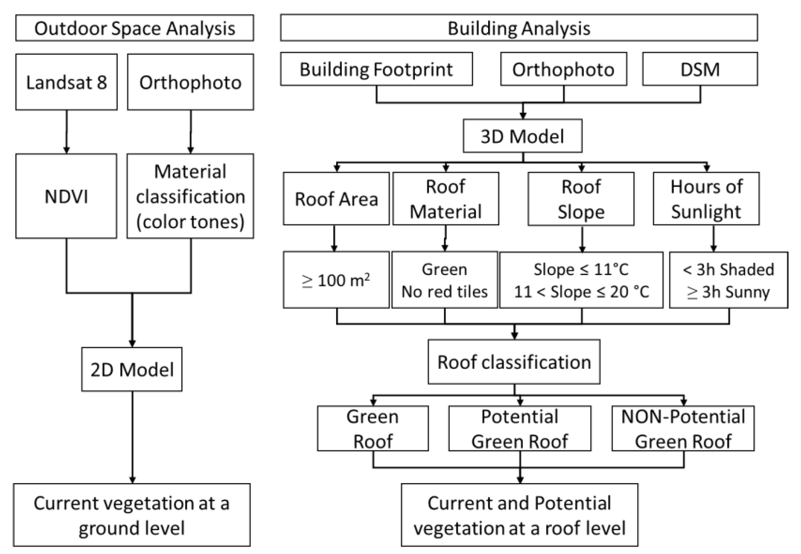
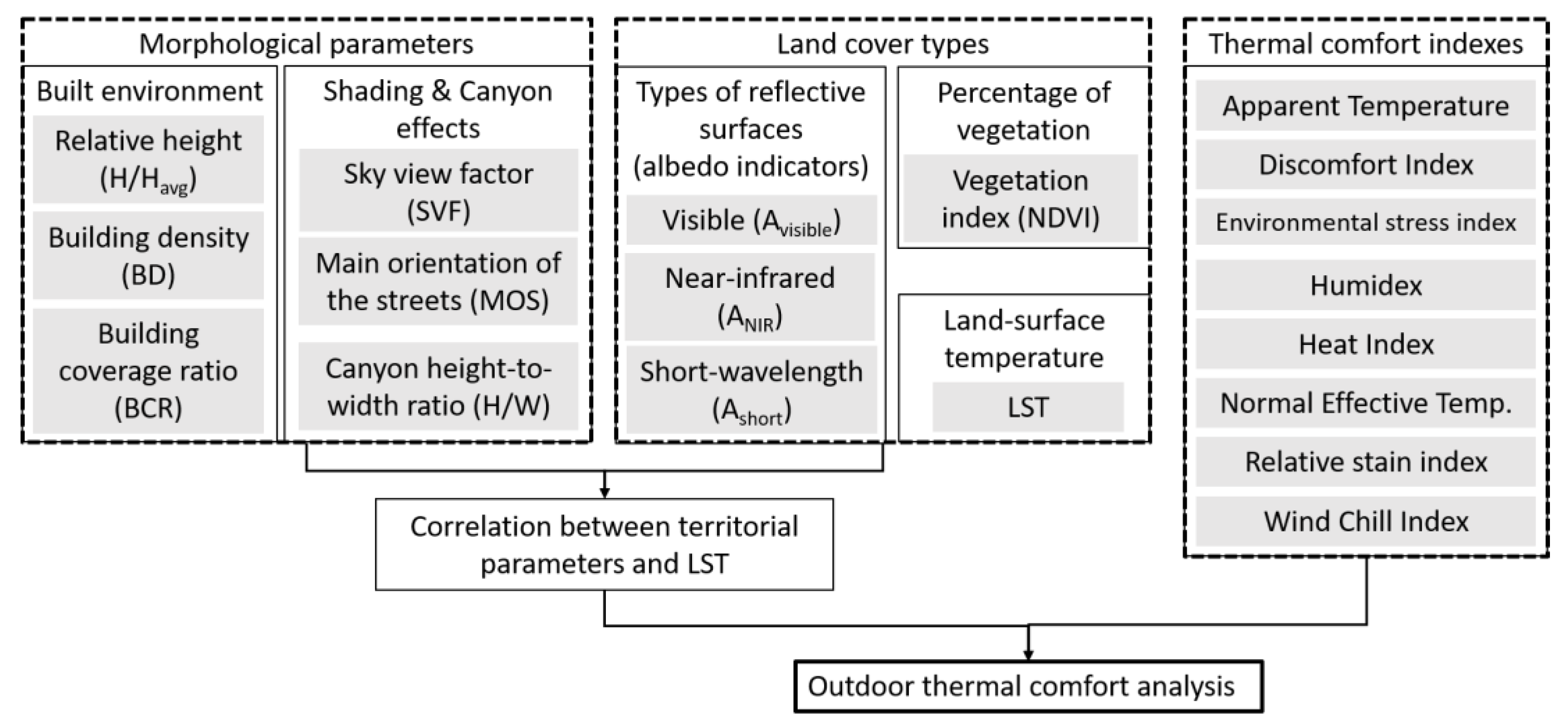
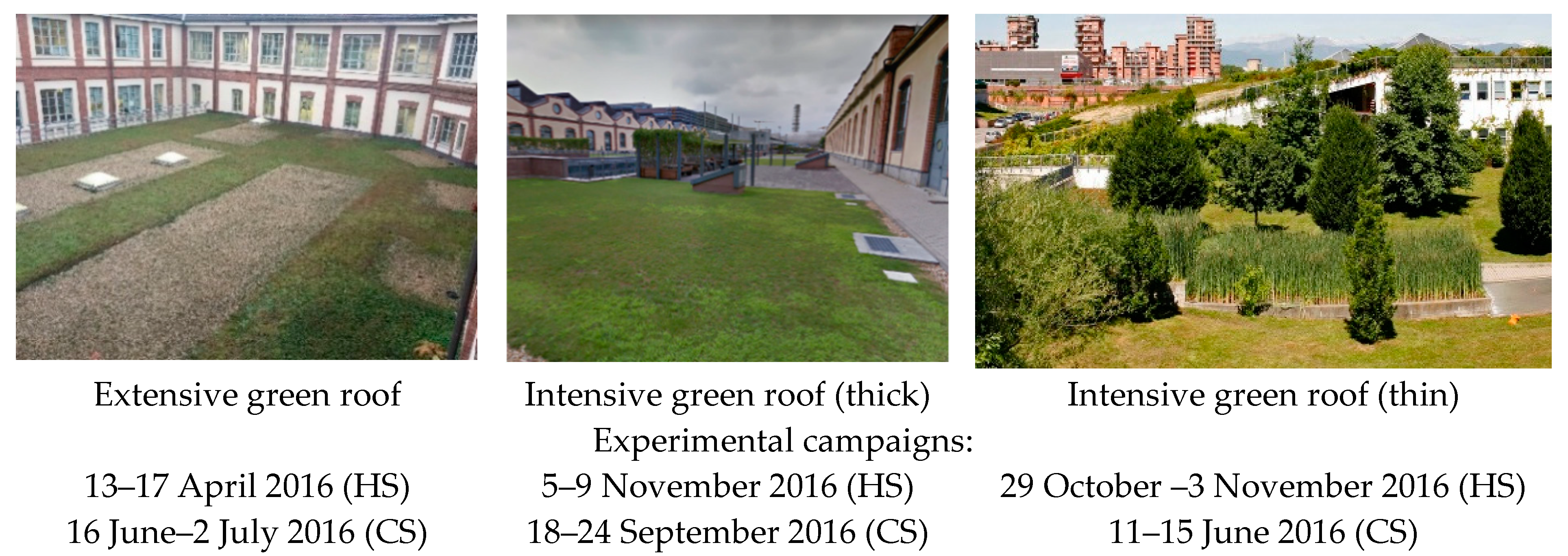
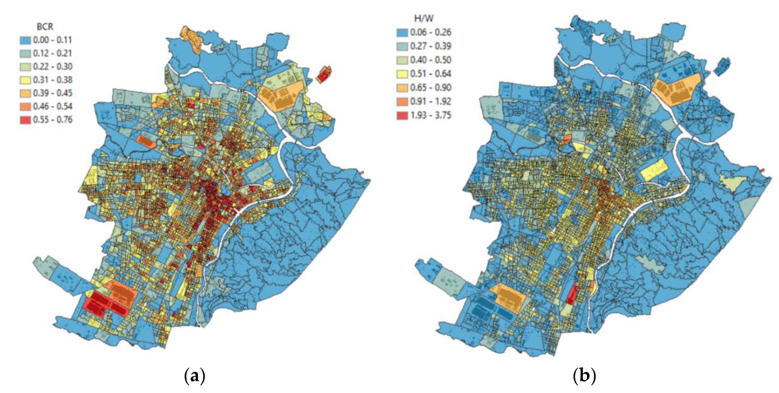
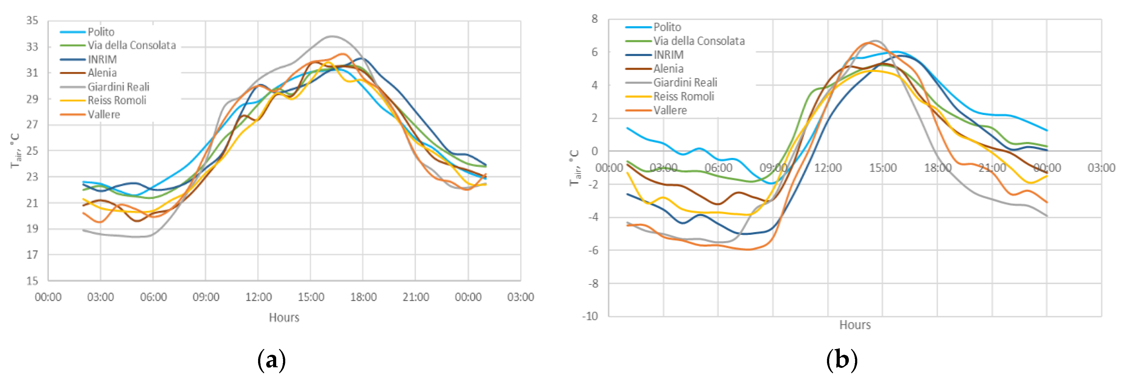
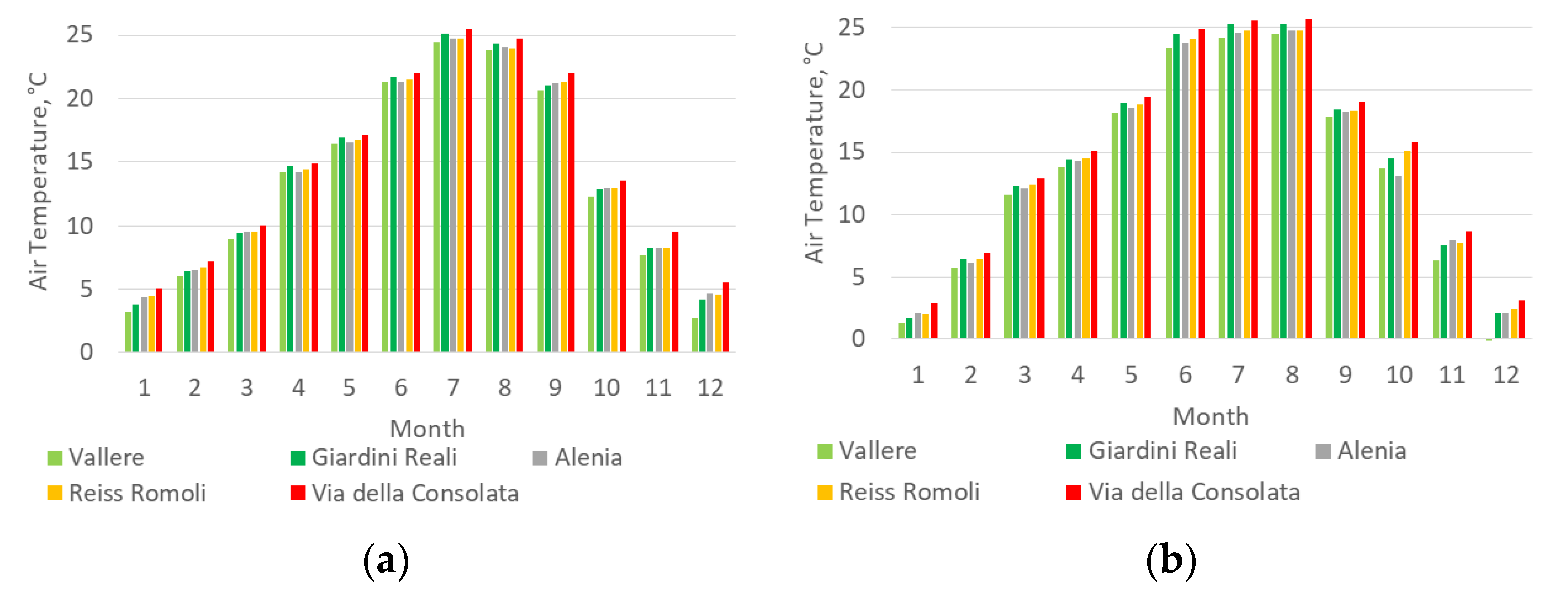
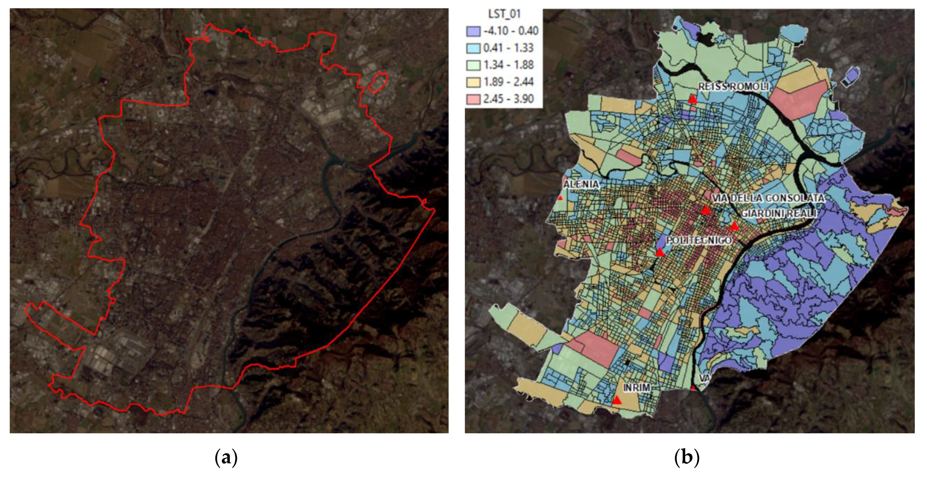
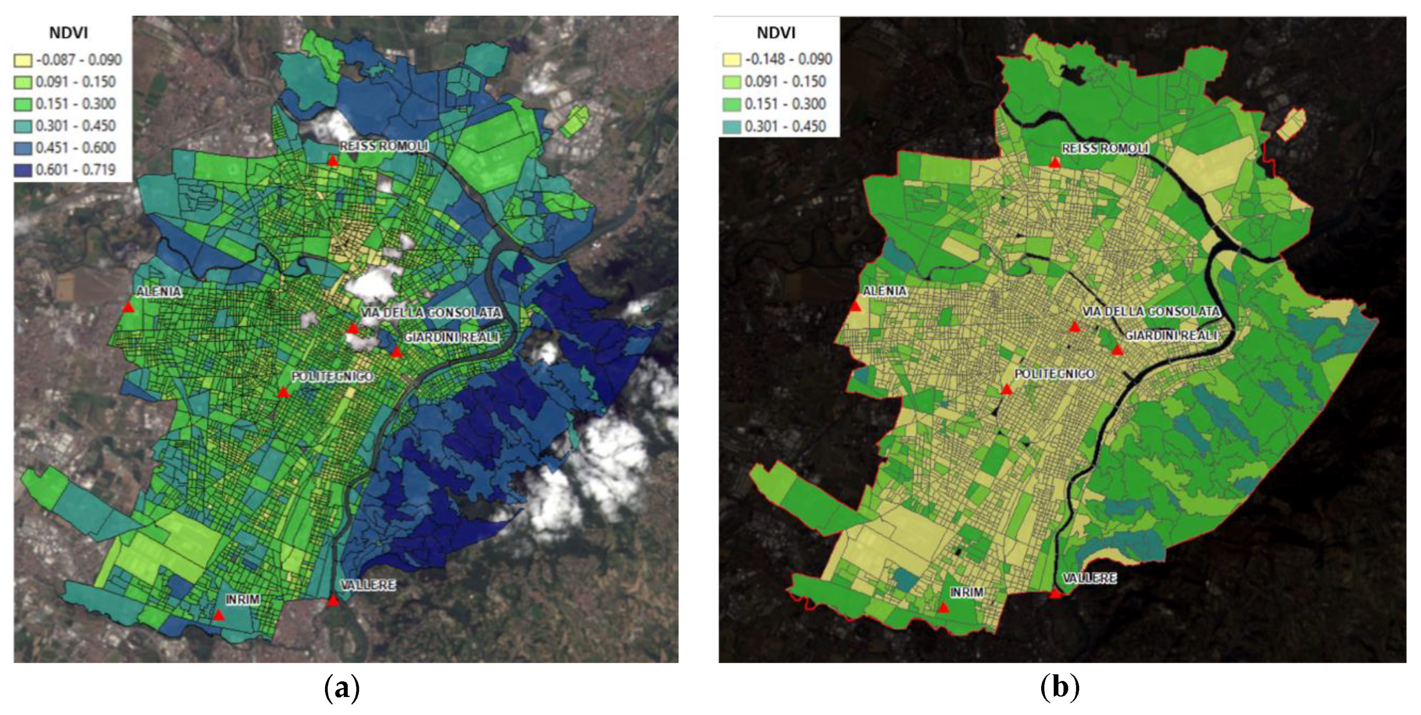
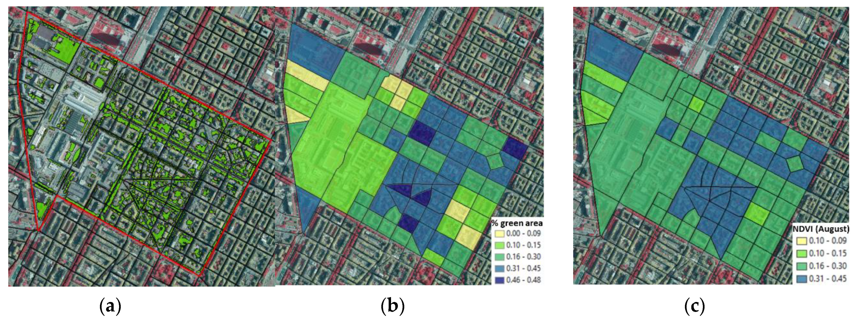
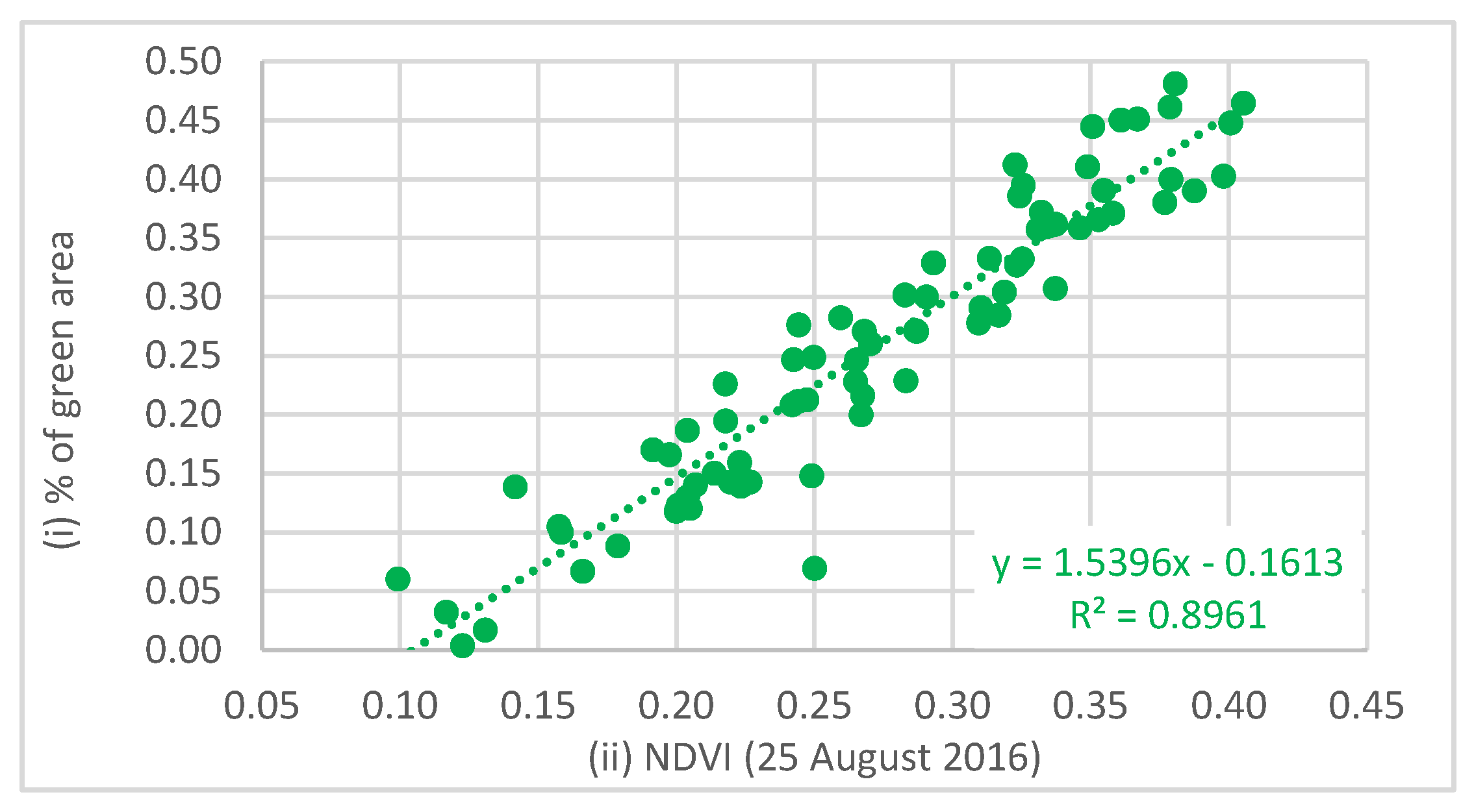
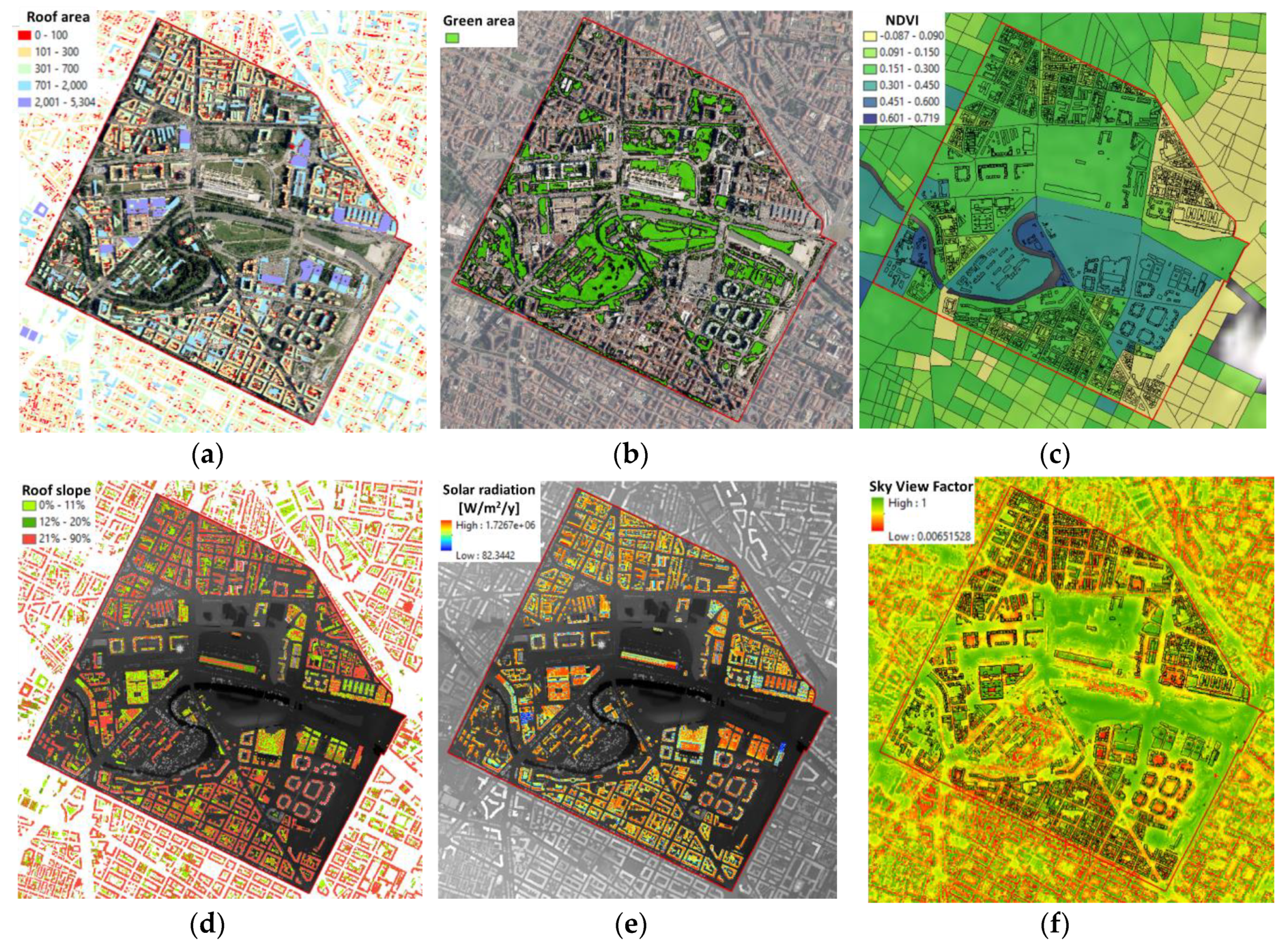
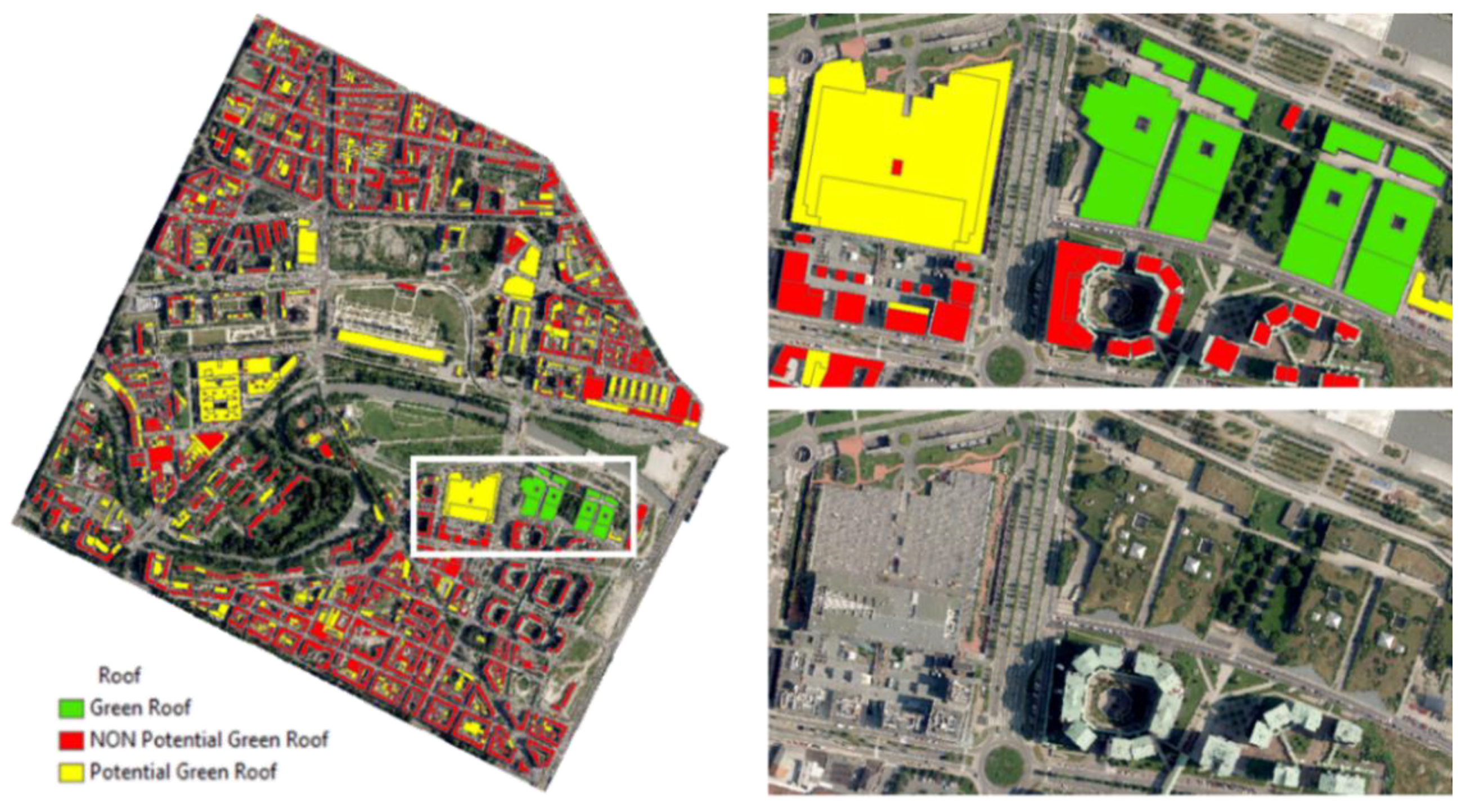
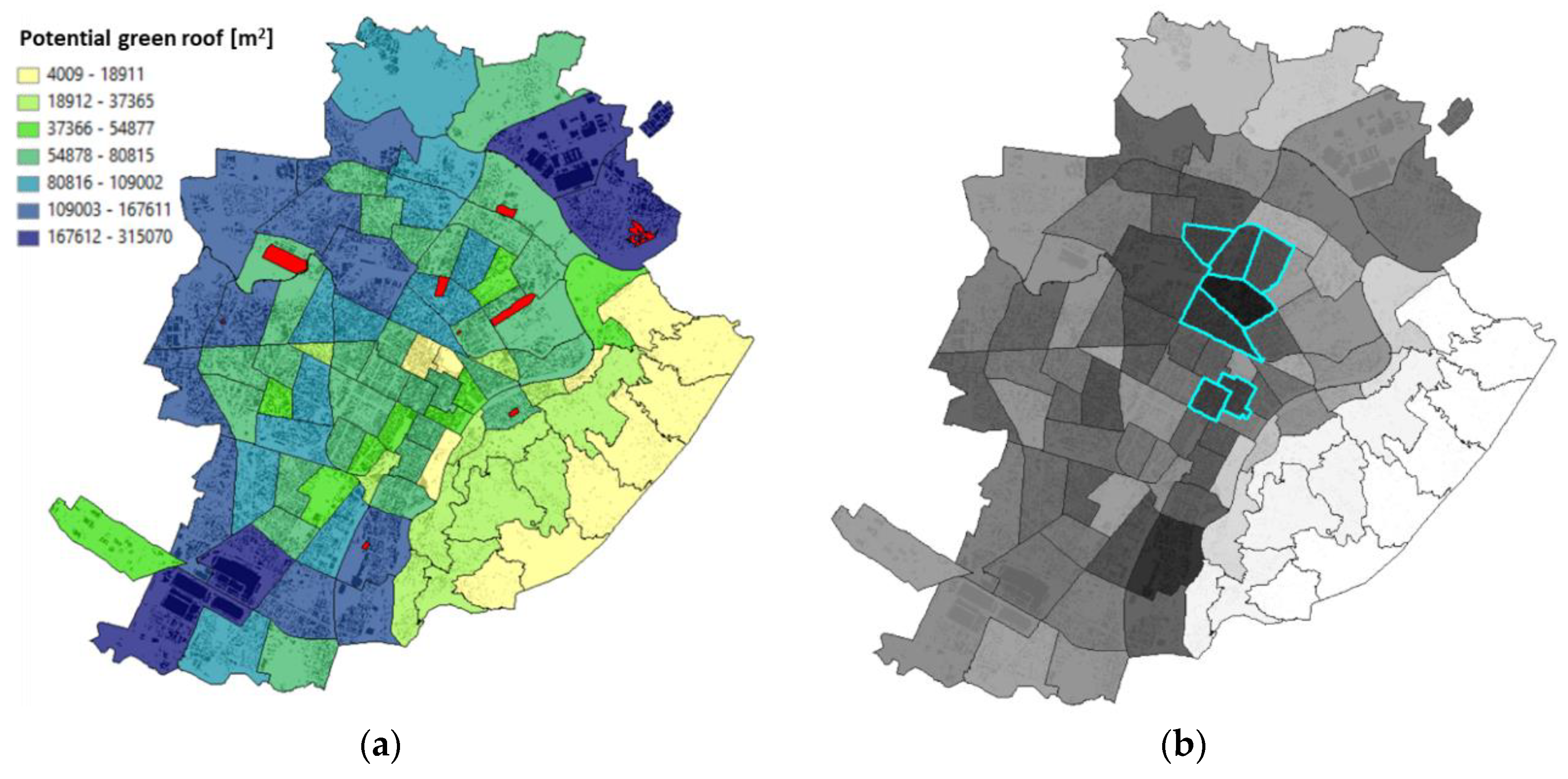
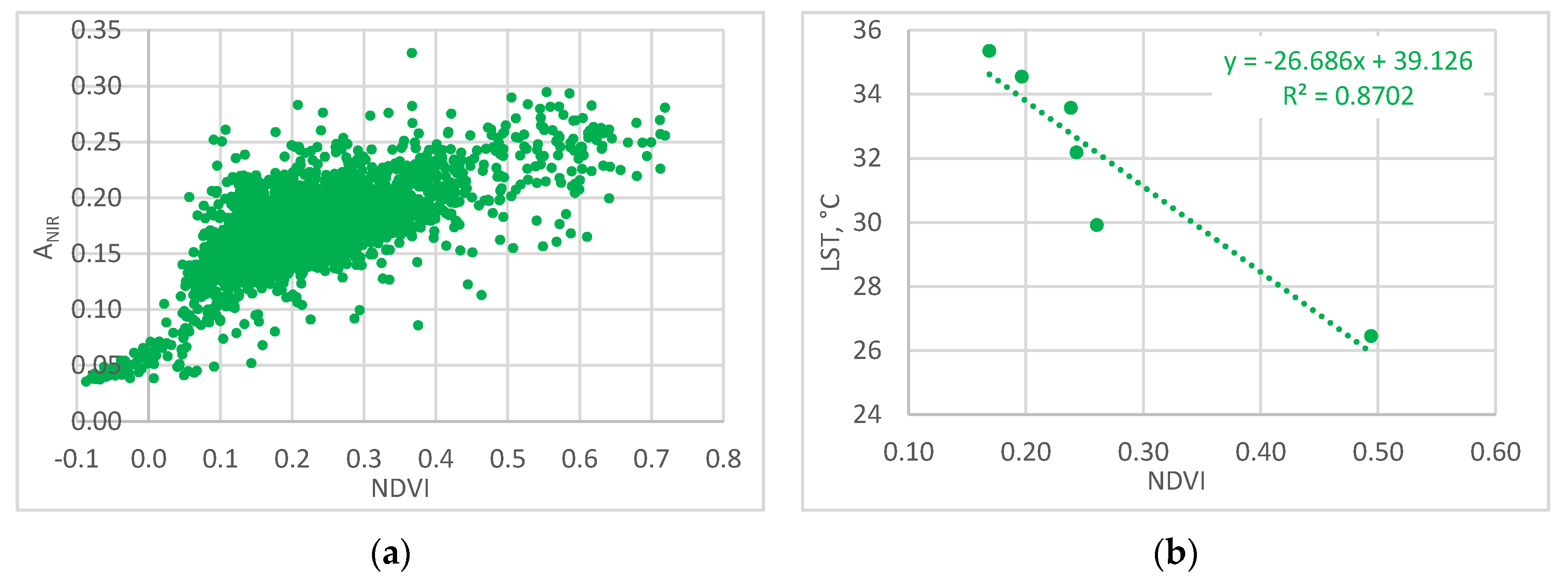
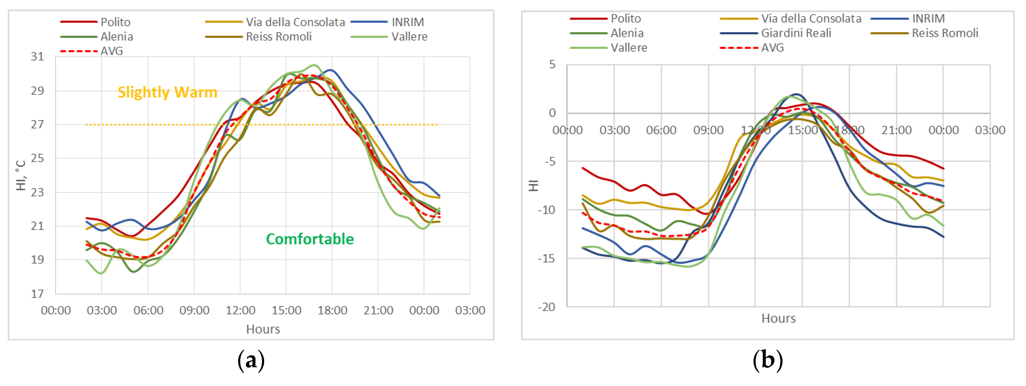
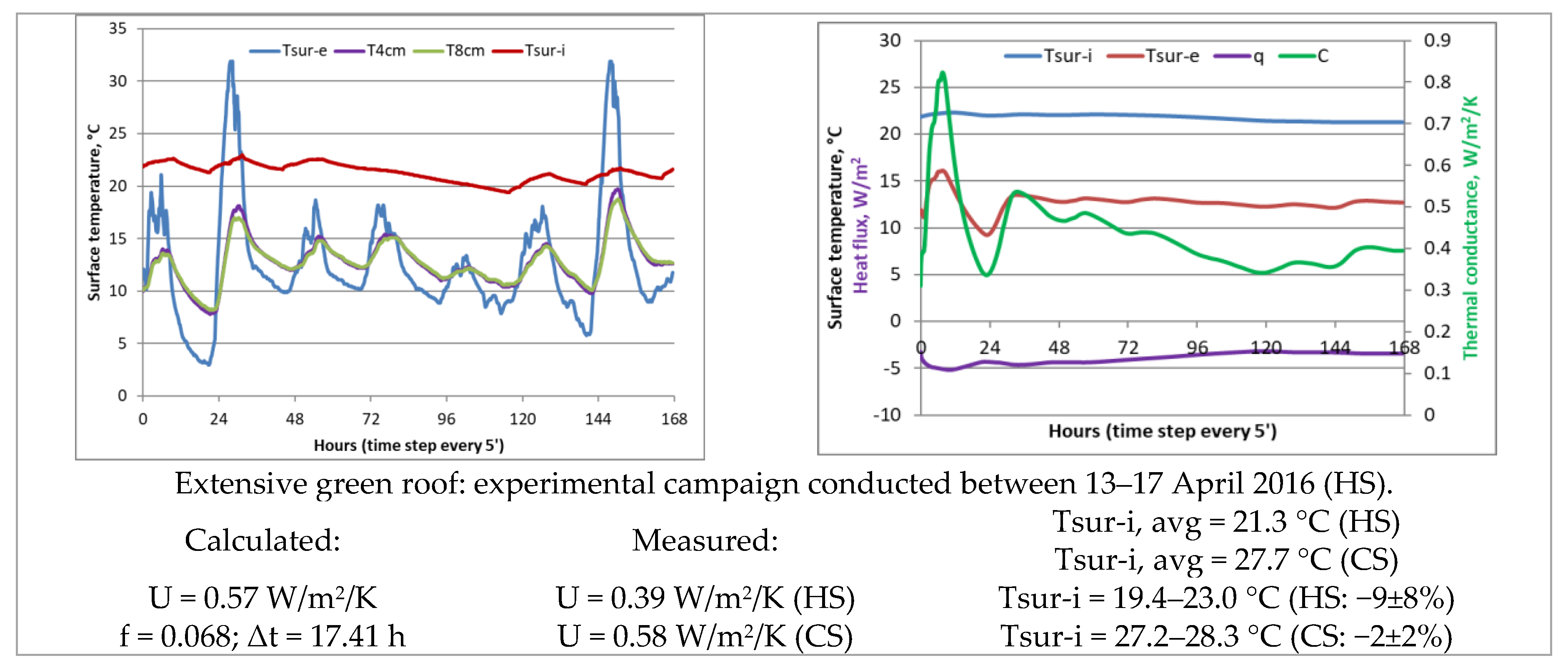
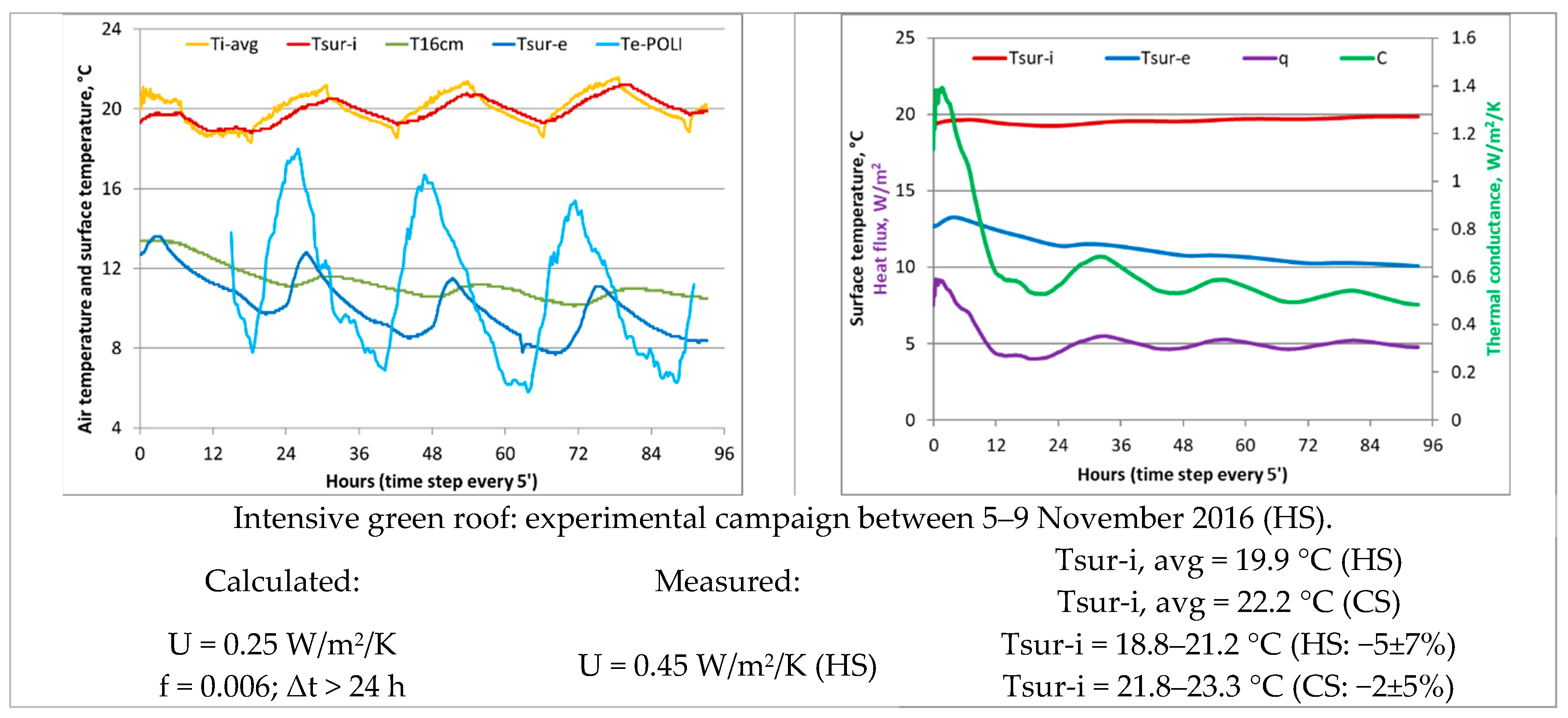
Table 1.
Literature review on the impact of green roofs and green urban areas on indoor and outdoor thermal comfort.
Table 1.
Literature review on the impact of green roofs and green urban areas on indoor and outdoor thermal comfort.
| Category | No. of Papers | Source |
|---|---|---|
| GIS-based methodology to evaluate green roofs and green urban areas | 9 | [4,5,6,7,8,9,10,11,12] |
| Outdoor thermal comfort: UHI mitigation strategies and thermal comfort indexes | 20 | [2,4,13,14,15,16,17,18,19,20,21,22,23,24,25,26,27,28,29,30] |
| Energy savings and Indoor thermal comfort from Green roofs | 5 | [1,31,32,33,34] |
Table 2.
Description of the data and their collection sources.
| Description | Type | Precision | Scale | Updated | Variables |
|---|---|---|---|---|---|
| Satellite images—Landsat 8 (OLI/TIRS) | raster | 30 m | Territorial | 21 January 2016, at 10:17 25 August 2016, at 10:11 | Avisible, Ashort, ANIR, NDVI, LST |
| Digital Surface Model (DSM) | raster | 0.5 m 5 m | Building | 2018 | Slope, solar radiation |
| Orthophotos | raster | 0.1 m | Building | 2018 | Land cover, type of materials |
| Municipal Technical Map | shapefile | - | Building/District | 2019 | m2, m3, BCR, BD, BH, H/W, MOS, SVF |
| Microclimate data—WSs | excel | Hourly | Point | From 1 January 2016 to 31 December 2016 | Tair, RH, vp, v, wind direction, SR |
Table 3.
Types of land cover with their relative NDVI values [36].
Table 3.
Types of land cover with their relative NDVI values [36].
| Land Cover | NDVI (−1, 1) |
|---|---|
| Thick vegetation | 0.6 < NDVI < 1 |
| Dense vegetation | 0.45 < NDVI < 0.6 |
| Medium vegetation | 0.3 < NDVI < 0.45 |
| Scarce vegetation | 0.15 < NDVI < 0.3 |
| Very scarce vegetation | 0.09 < NDVI < 0.15 |
| Bare ground | 0.025 < NDVI < 0.09 |
| Clouds | 0.002 < NDVI < 0.025 |
| Ice and snow | −0.046 < NDVI < 0.002 |
| Water | −1.00 < NDVI < −0.046 |
Table 4.
Thermal sensation scales of the outdoor comfort indexes: R = Reference, S = Sweltering, VH = Very Hot, H = Hot, W = Warm, SW = Slightly Warm, Cm = Comfortable, SC = Slightly Cool, C = Cool, Co = Cold, VC = Very Cold and EC = Extremely Cold.
Table 4.
Thermal sensation scales of the outdoor comfort indexes: R = Reference, S = Sweltering, VH = Very Hot, H = Hot, W = Warm, SW = Slightly Warm, Cm = Comfortable, SC = Slightly Cool, C = Cool, Co = Cold, VC = Very Cold and EC = Extremely Cold.
| Index | S | VH | H | W | SW | Cm | SC | C | Co | VC | EC |
|---|---|---|---|---|---|---|---|---|---|---|---|
| AT, °C | 40 | 40; 32 | 32; 27 | <27 | |||||||
| DI, °C | >26.5 | 26.4; 20 | 19.9; 15 | <14.9 | |||||||
| ESI, °C | >30 | 30; 28 | 28; 24 | 24; 18 | <18 | ||||||
| H, °C | >54 | 54; 45 | 45; 40 | 39; 30 | 29; 20 | <20 | |||||
| HI, °C | >54 | 54; 41 | 41; 32 | 32; 27 | <27 | ||||||
| NET, °C | >27 | 27; 23 | 23; 21 | 21; 17 | 14; 9 | 9; 1 | <1 | ||||
| RSI, - | ≥0.3 | <0.3 | |||||||||
| WCI, °C | >−10 | −10; −27 | −28; −39 | −40; −54 | <−55 | ||||||
Table 5.
Stratigraphy of the extensive green roof (thickness: 0.49 cm).
| Layers | Materials | Thickness | Density | Specific Heat | Thermal Conductivity (eq) |
|---|---|---|---|---|---|
| (from Outside to Inside) | (m) | (kg/m3) | (J/kg/K) | (W/m/K) | |
| 1 | Substrate | 0.12 | 1070 | 800 | 0.32 |
| 2 | Filter fabric | 0.001 | 930 | 2010 | 0.16 |
| 3 | Lapillo | 0.06 | 850 | 840 | 0.13 |
| 4 | Non-woven fabric protective layer | 0.001 | 930 | 2010 | 0.16 |
| 5 | Anti-root membrane | 0.004 | 920 | 2219 | 0.53 |
| 6 | Concrete lightened slab | 0.3 | 1110 | 880 | 0.40 |
Table 6.
Stratigraphy of the intensive thick (thickness: 0.91 cm) green roof.
| Layers | Materials | Thickness | Density | Specific Heat | Thermal Conductivity (eq) |
|---|---|---|---|---|---|
| (from Outside to Inside) | (m) | (kg/m3) | (J/kg/K) | (W/m/K) | |
| 1 | Substrate | 0.20 | 1200 | 2000 | 1.74 |
| 2 | Non-woven geotextile filter | 0.001 | 930 | 2010 | 0.16 |
| 3 | Lapillo | 0.15 | 850 | 840 | 0.20 |
| 4 | Drainage panels | 0.006 | 930 | 2010 | 0.16 |
| 5 | Anti-root membrane | 0.002 | 920 | 2219 | 0.53 |
| 6 | Non-woven separation | 0.001 | 930 | 2010 | 0.16 |
| 7 | Expanded polystyrene | 0.10 | 35 | 1250 | 0.04 |
| 8 | Bituminous mantle | 0.002 | 1200 | 920 | 0.17 |
| 9 | Screed slope | 0.12 | 400 | 1000 | 0.72 |
| 10 | Concrete slab | 0.34 | 2000 | 880 | 1.20 |
Table 7.
Stratigraphy of the intensive thin (thickness: 0.58 cm) green roof.
| Layers | Materials | Thickness | Density | Specific Heat | Thermal Conductivity (eq) |
|---|---|---|---|---|---|
| (from Outside to Inside) | (m) | (kg/m3) | (J/kg/K) | (W/m/K) | |
| 1 | Substrate | 0.16 | 1200 | 2000 | 1.74 |
| 2 | Polypropylene filter fabric | 0.005 | 930 | 2010 | 0.16 |
| 3 | Lapillo | 0.05 | 850 | 840 | 0.20 |
| 4 | Drainage layer | 0.004 | 920 | 2219 | 0.53 |
| 5 | Synthetic sheath | 0.002 | 1400 | 900 | 0.16 |
| 6 | Compensation non-woven fabric layer | 0.003 | 930 | 2010 | 0.16 |
| 7 | Expanded polystyrene | 0.05 | 35 | 1400 | 0.04 |
| 8 | Vapor barrier | 0.001 | 920 | 2219 | 0.53 |
| 9 | Concrete slab | 0.30 | 2000 | 880 | 1.20 |
Table 8.
Vegetation analysis conducted with the FA tool: percentage of green areas according to the RGB and IR orthophotos and urban variables values at census section scale (* satellite images refer to August 25th 2016, in brackets average value for the entire eight area).
Table 8.
Vegetation analysis conducted with the FA tool: percentage of green areas according to the RGB and IR orthophotos and urban variables values at census section scale (* satellite images refer to August 25th 2016, in brackets average value for the entire eight area).
| No | Zone (WS) | Total Area (m2) | Green Area (m2) | Green (%) | BCR (-) | H/Havg (-) | H/W (-) | MOS (-) | NDVI* (-) | ANIR * (-) | SVFg (-) | LST * (°C) |
|---|---|---|---|---|---|---|---|---|---|---|---|---|
| 1 | Reiss Romoli | 2,522,053 | 1,047,720 | 42 | 0.37 (0.26) | 0.96 (1.10) | 0.48 (0.26) | 0.79 (0.30) | 0.21 (0.23) | 0.23 (0.20) | 0.70 (0.62) | 34.9 (34) |
| 2 | EnviPark | 2,580,530 | 603,414 | 23 | 0.18 (0.34) | 0.98 (0.97) | 0.51 (0.41) | 0.61 (0.44) | 0.33 (0.16) | 0.21 (0.14) | 0.69 (0.53) | 31.4 (32) |
| 3 | Alenia | 2,023,227 | 615,188 | 30 | 0.37 (0.24) | 0.96 (1.02) | 0.20 (0.26) | 0.90 (0.56) | 0.20 (0.25) | 0.21 (0.21) | 0.66 (0.59) | 35.0 (33) |
| 4 | Via della Consolata | 526,163 | 32,114 | 6 | 0.45 (0.53) | 0.99 (0.97) | 0.77 (0.78) | 0.25 (0.44) | 0.11 (0.13) | 0.15 (0.26) | 0.44 (0.48) | 33.3 (32) |
| 5 | Giardini Reali | 301,124 | 114,642 | 38 | 0.01 (0.40) | 0.46 (0.87) | 0.19 (0.45) | 0.56 (0.46) | 0.48 (0.24) | 0.23 (0.20) | 0.58 (0.53) | 32.5 (34) |
| 6 | Politecnico | 1,283,824 | 297,560 | 23 | 0.31 (0.25) | 0.80 (0.97) | 0.25 (0.36) | 0.63 (0.27) | 0.16 (0.17) | 0.21 (0.51) | 0.66 (0.51) | 33.0 (33) |
| 7 | Vallere | 1,695,259 | 420,654 | 25 | 0.09 (0.27) | 1.01 (0.98) | 0.15 (0.36) | 0.76 (0.51) | 0.39 (0.19) | 0.19 (0.17) | 0.75 (0.55) | 31.3 (35) |
| 8 | Inrim | 1,752,786 | 663,758 | 38 | 0.08 (0.30) | 0.90 (0.98) | 0.20 (0.30) | 0.75 (0.40) | 0.42 (0.22) | 0.23 (0.19) | 0.67 (0.55) | 34.7 (36) |
| TURIN | 130,015,871 | 36,626,567 | 28 | 0.23 (0.33) | 0.88 (1.00) | 0.34 (0.41) | 0.66 (0.45) | 0.29 (0.21) | 0.21 (0.18) | 0.64 (0.51) | 33.3 (34) |
Table 9.
Identification of existing and potential green roofs in the eight areas of Turin.
| Area | Green Roof Classification | No. Buildings | % of Buildings | Roof Area [m2] | % of Roof Area |
|---|---|---|---|---|---|
| 1 | Existing green roof | 2 | 0.1% | 353 | 0.1% |
| Pitched potential roof | 49 | 2.5% | 17,829 | 4.4% | |
| Flat potential roof | 309 | 15.6% | 139,813 | 34.3% | |
| Non-potential green roof | 1625 | 81.9% | 249,964 | 61.3% | |
| 2 | Existing green roof | 16 | 0.5% | 24,579 | 4.0% |
| Pitched potential roof | 24 | 0.7% | 16,196 | 2.6% | |
| Flat potential roof | 355 | 10.7% | 154,022 | 25.1% | |
| Non-potential green roof | 2920 | 88.1% | 418,991 | 68.3% | |
| 3 | Existing green roof | 0 | 0.0% | 0 | 0.0% |
| Pitched potential roof | 49 | 2.5% | 17,829 | 4.5% | |
| Flat potential roof | 233 | 11.8% | 107,269 | 27.3% | |
| Non-potential green roof | 1688 | 85.7% | 267,830 | 68.2% | |
| 4 | Existing green roof | 0 | 0.0% | 0 | 0.0% |
| Pitched potential roof | 0 | 0.0% | 0 | 0.0% | |
| Flat potential roof | 34 | 2.7% | 9909 | 3.8% | |
| Non-potential green roof | 1220 | 97.3% | 251,818 | 96.2% | |
| 5 | Existing green roof | 0 | 0.0% | 0 | 0.0% |
| Pitched potential roof | 2 | 1.5% | 650 | 1.2% | |
| Flat potential roof | 6 | 4.6% | 4885 | 8.8% | |
| Non-potential green roof | 122 | 93.8% | 50,159 | 90.1% | |
| 6 | Existing green roof | 1 | 0.1% | 148 | 0.0% |
| Pitched potential roof | 7 | 0.5% | 2218 | 0.7% | |
| Flat potential roof | 122 | 8.2% | 56,276 | 17.2% | |
| Non-potential green roof | 1352 | 91.2% | 268,632 | 82.1% | |
| 7 | Existing green roof | 1 | 0.1% | 252 | 0.1% |
| Pitched potential roof | 18 | 1.5% | 8064 | 2.7% | |
| Flat potential roof | 202 | 16.5% | 118,737 | 40.0% | |
| Non-potential green roof | 1002 | 81.9% | 169,921 | 57.2% | |
| 8 | Existing green roof | 9 | 0.5% | 2185 | 0.8% |
| Pitched potential roof | 28 | 1.5% | 13,376 | 5.1% | |
| Flat potential roof | 174 | 9.1% | 58,688 | 22.4% | |
| Non-potential green roof | 1692 | 88.9% | 188,215 | 71.7% |
Table 10.
Urban parameters and land cover characteristics at a census section scale.
| Value | BCR | BD | BH | H/Havg | H/W | MOS | NDVI | ANIR | SVFg | LST |
|---|---|---|---|---|---|---|---|---|---|---|
| - | m2/m3 | - | - | - | - | - | - | - | °C | |
| Min. | 0.00 | 0.00 | 1.58 | 0.16 | 0.06 | 0.00 | 0.00 | 0.04 | 0.00 | 22.28 |
| Max. | 0.76 | 17.60 | 183.76 | 3.01 | 1.00 | 0.90 | 0.72 | 0.29 | 0.95 | 38.53 |
| Average | 0.33 | 4.94 | 18.23 | 1.00 | 0.40 | 0.45 | 0.21 | 0.17 | 0.51 | 33.97 |
| Median | 0.34 | 4.82 | 18.07 | 0.98 | 0.40 | 0.44 | 0.19 | 0.17 | 0.50 | 34.42 |
| St. dev. | 0.15 | 2.75 | 7.63 | 0.23 | 0.16 | 0.26 | 0.11 | 0.03 | 0.12 | 1.73 |
| Correl. with LST | 34% | 26% | 14% | 2% | 23% | 2% | −43% | −9% | −12% |
Table 11.
Aggregated data according to LST values (first column).
| LST | No. | BCR | BD | BH | H/Havg | H/W | MOS | NDVI | ANIR | SVFg | LST |
|---|---|---|---|---|---|---|---|---|---|---|---|
| °C | - | - | m2/m3 | - | - | - | - | - | - | - | °C |
| 22–27 | 48 | 0.09 | 1.30 | 13.15 | 1.03 | 0.22 | 0.45 | 0.49 | 0.20 | 0.61 | 26.45 |
| 28–29–30 | 224 | 0.24 | 2.98 | 13.28 | 0.97 | 0.32 | 0.45 | 0.26 | 0.15 | 0.59 | 29.92 |
| 31–32 | 412 | 0.29 | 4.31 | 17.12 | 1.01 | 0.37 | 0.43 | 0.24 | 0.17 | 0.53 | 32.18 |
| 33 | 652 | 0.31 | 4.91 | 19.40 | 1.03 | 0.40 | 0.44 | 0.24 | 0.18 | 0.50 | 33.57 |
| 34 | 1293 | 0.35 | 5.53 | 19.64 | 1.01 | 0.43 | 0.46 | 0.20 | 0.17 | 0.49 | 34.54 |
| 35 | 782 | 0.37 | 5.37 | 17.93 | 0.99 | 0.43 | 0.45 | 0.17 | 0.17 | 0.50 | 35.35 |
| 36–39 | 109 | 0.36 | 3.56 | 12.44 | 0.93 | 0.30 | 0.49 | 0.17 | 0.18 | 0.62 | 36.52 |
| Correl. with LST | - | 97% | 80% | 40% | −47% | 67% | 47% | −93% | −39% | −43% |
Table 12.
Energy, economic and emissions savings with green roofs.
| Scenario | Ubefore (W/m2/K) | Uafter (W/m2/K) | Energy Savings (MWh) | Economic Savings (M€) | GHG Emissions Avoided (tonCO2) | Hectares of Woods (ha) |
|---|---|---|---|---|---|---|
| 1 | 1.65 | 0.24 | 39,249 | 2.98 | 7968 | 79.7 |
| 2 | 0.97 | 0.24 | 20,321 | 1.54 | 4125 | 41.3 |
| 3 | 0.57 | 0.24 | 9186 | 0.70 | 1865 | 18.6 |
© 2020 by the authors. Licensee MDPI, Basel, Switzerland. This article is an open access article distributed under the terms and conditions of the Creative Commons Attribution (CC BY) license (http://creativecommons.org/licenses/by/4.0/).
Share and Cite
MDPI and ACS Style
Mutani, G.; Todeschi, V. The Effects of Green Roofs on Outdoor Thermal Comfort, Urban Heat Island Mitigation and Energy Savings. Atmosphere 2020, 11, 123. https://0-doi-org.brum.beds.ac.uk/10.3390/atmos11020123
AMA Style
Mutani G, Todeschi V. The Effects of Green Roofs on Outdoor Thermal Comfort, Urban Heat Island Mitigation and Energy Savings. Atmosphere. 2020; 11(2):123. https://0-doi-org.brum.beds.ac.uk/10.3390/atmos11020123
Chicago/Turabian StyleMutani, Guglielmina, and Valeria Todeschi. 2020. "The Effects of Green Roofs on Outdoor Thermal Comfort, Urban Heat Island Mitigation and Energy Savings" Atmosphere 11, no. 2: 123. https://0-doi-org.brum.beds.ac.uk/10.3390/atmos11020123
Note that from the first issue of 2016, this journal uses article numbers instead of page numbers. See further details here.