Characterization of Wind-Sea- and Swell-Induced Wave Energy along the Norwegian Coast

Abstract

The necessity to reduce $C{O}_2$ emissions in combination with the rising energy demand worldwide makes the extensive use of renewable energy sources increasingly important. To that end, countries with long coastlines, such as Norway, can exploit ocean wave energy to produce large amounts of power. In order to facilitate these efforts as well as to provide quantitative data on the wave energy potential of a specific area, it is essential to analyze the weather and climatic conditions detecting any variabilities. The complex physical processes and the atmosphere-wave synergetic effects make the investigation of temporal variability of wave energy a challenging issue. This work aims to shed new light on potential wave energy mapping, presenting a spatio-temporal assessment of swell- and wind-sea-induced energy flux in the Nordic Seas with a focus on the Norwegian coastline using the NORA10 hindcast for the period 1958–2017 (59 years). The results indicate high spatial and seasonal variability of the wave energy flux along the coast. The maximum wave energy flux is observed during winter, while the minimum is observed during summer. The highest coastal wave energy flux is observed in the Norwegian Sea. The majority of areas with dominant swell conditions (i.e., in the Norwegian Sea) are characterized by the highest coastal wave energy flux. The maximum values of wave energy flux in the North Sea are denoted in its northern parts in the intersection with the Norwegian Sea. In contrast to the Norwegian Sea, areas located in the North Sea and the Barents Sea show that wind sea is contributing more than swell to the total wave energy flux.

1. Introduction

According to the European long-term strategy [1], Europe needs to maximize the deployment of renewables aiming to fully decarbonize its energy supply. Marine Renewable Energy (MRE) resources such as wind, tidal currents, and waves could play a key role in the decarbonization of electricity production around the world [2]. Globally, there are many offshore areas characterized by considerably high marine energy supply, due to intense winds, increased tidal activity, and high waves [3]. The oceans offer a vast amount of renewable energy that is currently unexploited. Thus, the accurate estimation of the MRE potential is fundamental in harnessing ocean energy. This will provide a design basis for the development of innovative technologies to overcome current constraints in renewable energy production in terms of efficiency and damage prevention. In this context, there is an increasing interest among the scientific community to quantify the potential of global MRE resources and to analyze their economic aspect, while advancing their technology [4,5,6,7,8,9,10,11,12]. Moreover, as MRE production is highly dependent on weather conditions, the aspect of climatic variability is a critical factor for a realistic assessment of energy potential. It has been concluded by Reguero et al. [13] that the anthropogenic upper-ocean warming is changing the global wave climate, making waves stronger and, overall, increasing wave power globally by $0.4\%$ per year. Countries with long coastlines facing the Atlantic Ocean, such as Norway, are characterized by large amounts of MRE potential [14] in the form of wave energy. The deployment of large-scale wave power plants requires high-quality quantification of the wave energy potential resource [15], as the detailed assessment of wave energy potential can reveal areas characterized by significant wave energy potential. Areas with pre-existing wind power plants can be good candidates for the installation of wave energy plants to increase production efficiency and decrease in costs (since the existing infrastructure and distribution network will be reused) [5]. This will also result in diversified energy supply plants that are less vulnerable to wind and wave variabilities. Concerning the Norwegian coast, several ocean-wave energy studies have been carried out since 1970, estimating the average wave power between 20 and 41 kW m${}^{-1}$ [16]. A modeling study on potential sites for offshore energy exploitation was conducted by Kalogeri et al. [17], and it was concluded that the coasts of Norway were among the best spots for this kind of development. Even though hydropower is the main energy resource in Norway [4,18,19], the wave energy potential is large enough to cover domestic demand as well as export production surplus to neighboring countries in accordance with the European energy megagrid [20]. Consequently, a detailed estimation of the spatiotemporal variabilities of wave energy potential along the Norwegian coastlines is of high significance, not only on a regional but also on a European scale.

In this context, this study presents spatial and seasonal analyses of the wave energy flux in the North Sea, the Norwegian Sea, and the Barents Sea. Wave energy converters, the devices used to transform kinetic and potential energy of waves to electricity, respond differently to low- and high-frequency waves. The swell waves are more significant in the wave energy converter industry because the wave energy density is more consistent over a year [21]. For this reason, wave energy fluxes due to swell and wind sea are examined individually in this study. It is noteworthy that complex physical processes and atmosphere–wave synergetic effects affecting wave energy flux are usually investigated using either two-way atmosphere–wave coupled modeling systems [22,23,24] or high-resolution reanalysis/hindcast data. For instance, a global ocean wave energy resource based on ERA-40 wave reanalysis data was analyzed by Zheng et al. [25], and global ocean energy was estimated by Cornett [26] using a WAVEWATCHIII [27] hindcast. Hence, in order to perform our analysis, the regional NORA10 hindcast was employed including swell and wind sea data for the period 1958–2017 (59 years). NORA10 covers the North Sea, the Norwegian Sea, and the Barents Sea in a fine horizontal resolution of 10–11 km [28]. The NORA10 dataset was found to be in good agreement when compared against observations [28,29]. The resulting time series of wave energy fluxes were analyzed to characterize 10 selected offshore areas. The main focus of the study is the characterization of wave energy flux due to swell and wind sea along the Norwegian coast. Our analysis aims to give a comprehensive assessment of wave energy flux and to identify areas with high wave energy potential along the Norwegian coast.

This paper is organized as follows. Section 2 is dedicated to materials and methods. Section 3 describes the wave climate in the Northeast Atlantic and along the Norwegian coast. The discussion of the results is presented in Section 4. Finally, Section 5 provides the conclusions.

2. Materials and Methods

The NORA10 (Norwegian Reanalysis Archive 10 km) hindcast includes various atmospheric and wave data for the Northeast Atlantic, including the North Sea, the Norwegian Sea, and the Barents Sea. It has a horizontal grid resolution and a time interval of 0.1${}^{\circ }$× 0.1${}^{\circ }$ and 3 h, respectively [28]. It is developed by the Norwegian Meteorological Institute combining atmospheric and wave modeling techniques. They performed dynamical atmospheric downscaling of the European Centre for Medium-Range Weather Forecasts (ECMWF) ERA-40 [30] reanalysis data using the 10-km High-Resolution Limited Area Model (HIRLAM; Undén et al. [31]); consequently, they forced the wave model WAM cycle 4 [32] with surface wind fields produced by the HIRLAM model (more information in Reistad et al. [28]). As the ERA-40 dataset has been available since 2002, NORA10 is continually being extended using operational analyses from the ECMWF as boundary and initial conditions [28,33]. It is important to note that NORA10 was compared by Aarnes et al. [33] to wave observations in the North Sea and the Norwegian Sea during the period 1958–2009, and it was ensured that NORA10 does not possess a discontinuity of significance before and after 2002. Hence, we used the continuous 59-year period from January 1958 to December 2017. In order to cover a sufficient part of offshore areas along the Norwegian coastline, we selected 10 representative points (Figure 1). The data subsets representing the 10 points consist of significant wave heights and wave periods for both swell and wind sea, facilitating the scope of this study.

The Wave Energy Flux (WEF) is given by Equation (1) [34]:

$$WEF={\rho }_{w}g{\int }_0^{2\pi }{\int }_0^{\infty }{c}_g(f,z)S(f,\theta )dfd\theta$$

(1)

where $S(f,\theta )$ is the directional wave energy spectrum, f is the wave frequency, $\theta$ is the wave propagation direction, ${\rho }_w$ is the seawater density, g is the gravitational acceleration, and $c_g$ is the group velocity, i.e., the velocity at which wave energy propagates, which is a function of the wave frequency and water depth (z). Even though seawater density depends on salinity and temperature, which vary in time and space, an average value is set for this work, ${\rho }_w$ = 1025 kg m${}^{-3}$, as also used by Iglesias et al. [34]. Considering deep waters, the wave energy flux, expressed in kW per meter of wave crest length (kW m${}^{-1}$), is approximately estimated following Equation (2) ([35,36,37,38,39] for total WEF):

$$WEF=\frac{{\rho }_w{g}^2}{64\pi }{H}_s^2{T}_e\left\{\begin{array}{c}WE{F}_s=\frac{{\rho }_w{g}^2}{64\pi }{H}_{s,s}^2{T}_{e,s}\hfill \\ WE{F}_w=\frac{{\rho }_w{g}^2}{64\pi }{H}_{s,w}^2{T}_{e,w}\hfill \end{array}\right.$$

(2)

where $H_s$ is the total significant wave height (m), $H_{s,s}$ is the swell component of significant wave height (m), $H_{s,w}$ is the wind sea component of significant wave height (m), $T_e$ is the total wave energy period (s), $T_{e,s}$ is the swell component of wave energy period (s), and $T_{e,w}$ is the wind sea component of wave energy period (s). Total WEF as well as wind-sea-induced ($WE{F}_w$) and swell-induced ($WE{F}_s$) wave energy flux can be estimated using the respective significant wave height and wave energy period in Equation (2). Based on the WAM model, the wave components that are not subject to wind forcing are defined as swell, while the rest are defined as wind sea [32]. The significant wave height is defined by Equation (3):

$$H_s=4\sqrt{m_0}$$

(3)

where $m_0$ is the zeroth moment (the variance) of the wave spectrum [40]. The spectral moments are defined by Equation (4):

$$m_n={\int }_0^{2\pi }{\int }_0^{\infty }{f}^{n}S(f,\theta )dfd\theta ,n=0,1,2,3\dots$$

(4)

where $S(f,\theta )$ is the spectral density as a function of frequency (f) and direction ($\theta$).

The following relation between wave energy and peak wave period ($T_p$) was proposed by Cahill and Lewis [41] assuming a Bretschneider spectrum:

$$T_e=0.85T_p$$

(5)

Since $T_e$ was not available in the NORA10 dataset, we adopted Equation (5) in order to approximate the wave energy period used in Equation (2) for total WEF as well as swell- and wind-sea-induced WEF. The use of a relation including peak spectral wave period instead of the actual wave energy period should not impact significantly the results of a spatio-temporal analysis of wave energy. Regarding the computation of $WEF$, in Santo et al. [42] and Varlas et al. [43], the $T_p$ was used instead of $T_e$, while in Sasaki [44], the significant wave period ($T_s$) was employed. In Goddijn-Murphy et al. [45], the zero-crossing period ($T_z$) was used to estimate the energy period ($T_e=1.18T_z$, adapted by [41]). Similar to our analysis, Cornett [26], Bento et al. [38] and Boronowski et al. [46] computed $T_e$ according to $T_e=0.9T_p$ for wave energy estimations.

In the following section, the seasonal and spatial variability of WEF resources, induced by wind sea and swell, is analyzed for the Nordic Seas and along the Norwegian coast (10 selected points). Finally, for the estimation of WEF-distribution by direction (WEF-rose) along the Norwegian coast, we used the mean direction for total WEF-rose and the peak direction of wind sea and swell for $WE{F}_w$- and $WE{F}_s$-rose.

3. Results

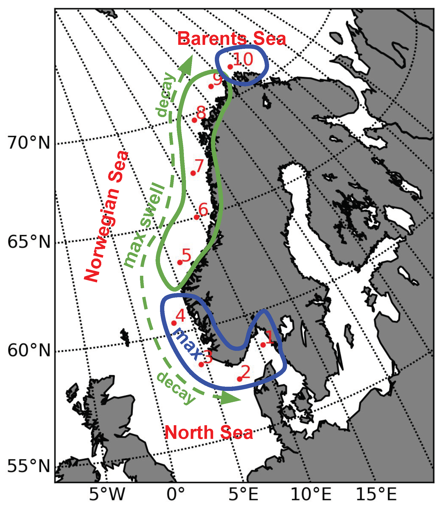
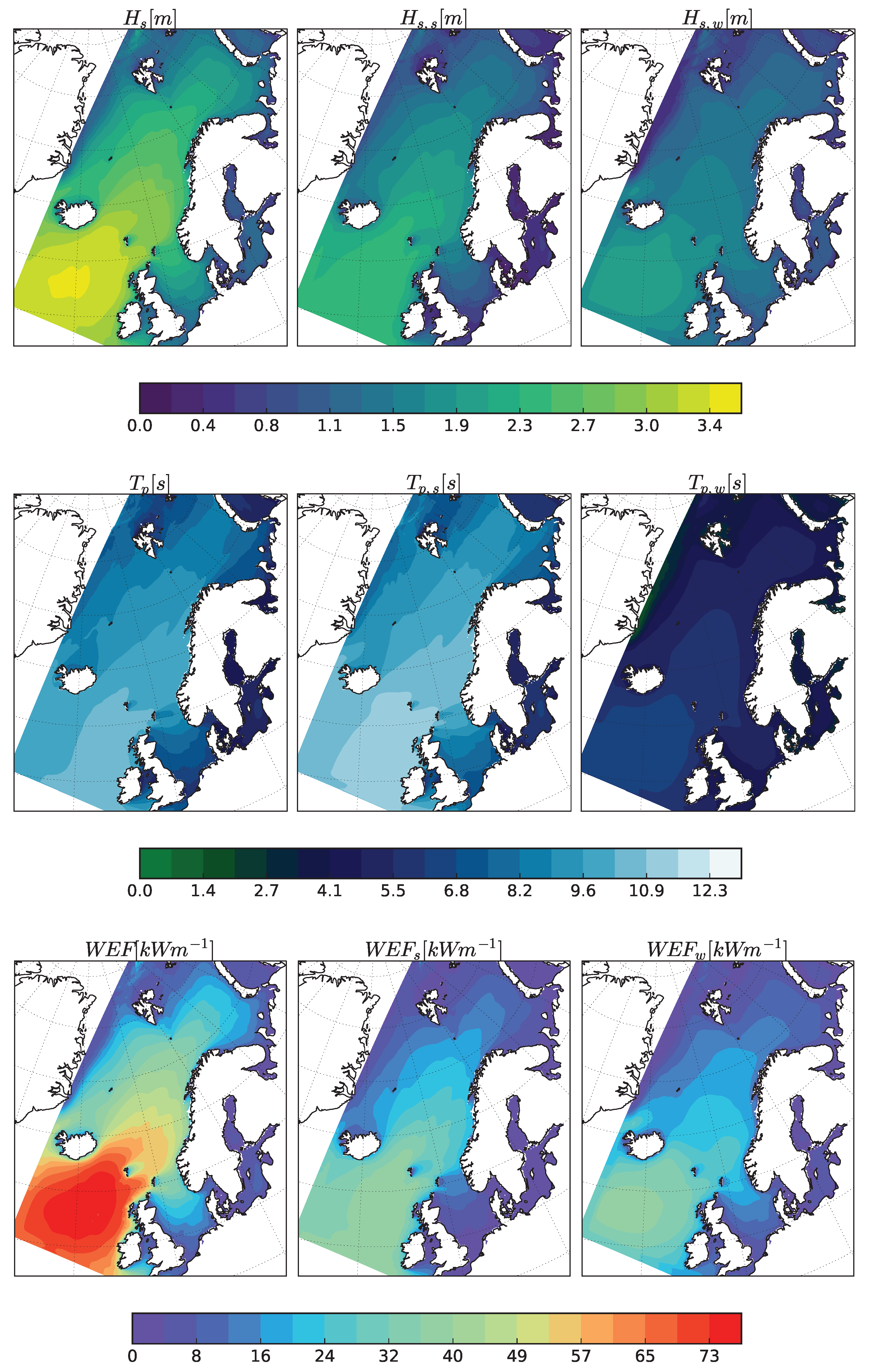
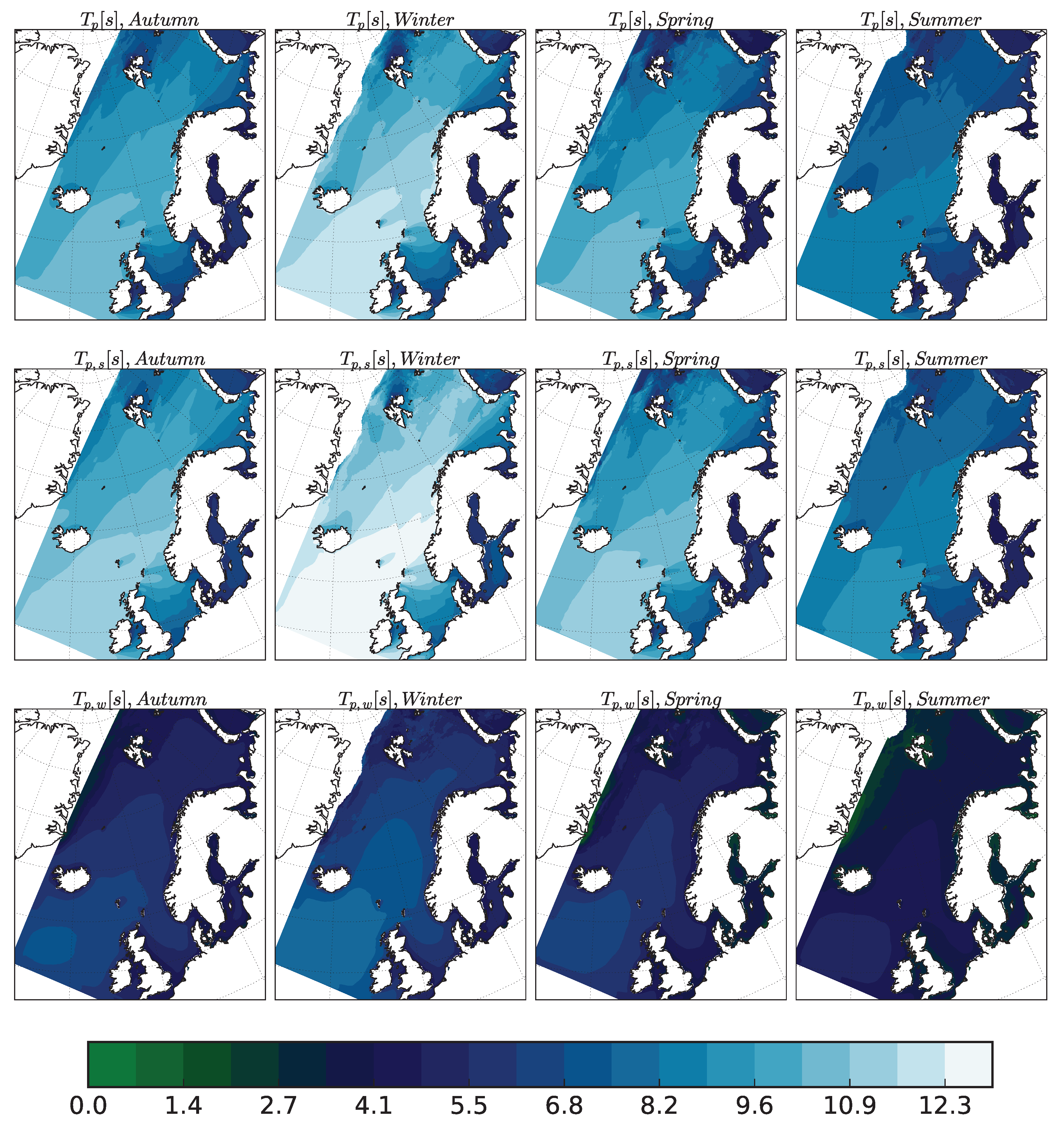
3.1. Wave Climate in the Northeast Atlantic: The North Sea, the Norwegian Sea, and  the Barents Sea

This section presents the average total WEF for the period from 1958 to 2017 (59 years) as well as the contribution of wind sea and swell in WEF. The results are based on the methodology presented in the previous section.

The spatial variation of the average $H_s$, $T_p$, and $WEF$ values is shown in Figure 2 for NORA10 domain covering the Northeast Atlantic Ocean including the Nordic Seas i.e., the North Sea, the Norwegian Sea, and the Barents Sea. The highest values of $H_s$, $T_p$, and $WEF$ were observed in the area in the Northwest of Ireland. $H_s$, $H_{s,s}$, and $H_{s,w}$ reached 3.6, 2.5, and 2.3 m, respectively. The peak wave period $T_p$ reached 11.5 s, while $T_{p,s}$ and $T_{p,w}$ reached 12.5 and 7 s, respectively. Regarding the wave energy fluxes, $WEF$, $WE{F}_s$, and $WE{F}_w$ reached 77, 44, and 44 kW m${}^{-1}$, respectively.

Moreover, we observed relatively low values of $H_s$, $T_p$, and $WEF$ in the North Sea. This is attributed to the fact that the North Sea is less exposed to high waves and swell due to sheltering by the British Isles. Hence, $H_s$ ranged from 0.5 to 2.5 m, while $H_{s,s}$ and $H_{s,w}$ ranged from 0.5 to 1.9 m and from 0.5 to 2.1 m, respectively. As far as the peak wave periods are concerned, $T_p$, $T_{p,s}$, and $T_{p,w}$ ranged from 5 to 9 s, from 6 to 11 s, and from 3 to 7 s, respectively. It is noteworthy that the highest wave periods were observed at the Northern parts of the North Sea in the intersection with the Norwegian Sea. The low values of both significant wave height and wave period in the North Sea led to low WEF values, $WEF$$<40$ kW m${}^{-1}$, $WE{F}_s$$<20$ kW m${}^{-1}$ and $WE{F}_w$$<20$ kW m${}^{-1}$.

In contrast to the North Sea, the Norwegian Sea was exposed directly to high waves from the North Atlantic Ocean, leading to higher values of $H_s$ and $T_p$ and, subsequently, of $WEF$. Therefore, $H_s$ ranged from 2.4 to 3.2 m, while $H_{s,s}$ and $H_{s,w}$ ranged from 1.5 to 1.9 m and from 1.3 to 1.7 m, respectively. Furthermore, $T_p$, $T_{p,s}$, and $T_{p,w}$ ranged from 9 to 12 s, from 9.5 to 12 s, and from 5 to 6 s. Regarding the WEF values, $WEF$ ranged from 30 to 57 kW m${}^{-1}$, while $WE{F}_s$ was lower than 32 kW m${}^{-1}$, and $WE{F}_w$ was lower than 28 kW m${}^{-1}$.

The Barents Sea was characterized by lower values of $H_s$, $T_p$, and $WEF$ compared to the Norwegian Sea. Thus, $H_s$ ranged from 1.0 to 2.5 m, while $H_{s,s}$ ranged from 0.5 to 1.9 m, and $H_{s,w}$ was higher than 0.5 and lower than 1.5 m. Accordingly, $T_p$ ranged from 6 to 9 s, while $T_{p,s}$ and $T_{p,w}$ ranged from 6 to 10 s and from 4 to 6 s, respectively. Concerning WEF values, $WEF$ was demonstrated up to 36 kW m${}^{-1}$, while $WE{F}_s$ and $WE{F}_w$ reached 20 kW m${}^{-1}$, respectively.

In order to investigate the seasonal variations of wave parameters in the Northeast Atlantic Ocean, we estimated the average total, swell, and wind sea component of $H_s$, $T_p$, and WEF for autumn (September, October, and November), winter (December, January, and February), spring (March, April, and May), and summer (June, July, and August), as illustrated in Figure 3, Figure 4 and Figure 5. During the winter season, the wave height had the highest values. In more detail, $H_s$ northeast of Ireland reached 5 m, while $H_{s,s}$ and $H_{s,w}$ were up to 3.4 and 3.2 m, respectively. In the North Sea, $H_s$, $H_{s,s}$, and $H_{s,w}$ were about 3.7, 2.6, and 2.6 m. In the Norwegian Sea, $H_s$ reached 4.2 m, while $H_{s,s}$ and $H_{s,w}$ reached 2.9 and 2.4 m, respectively. Moreover, in the Barents Sea, $H_s$, $H_{s,s}$, and $H_{s,w}$ reached 2.8, 1.6, and 1.3 m, respectively. The autumn season was characterized by about 1 m lower values of $H_s$, $H_{s,s}$, and $H_{s,w}$ than winter. Spring showed reduced values in comparison with autumn, while summer was the season with the lowest wave heights. Regarding the peak wave period, during winter, we observed the highest values with $T_p$ = 11.5 s, $T_{p,s}$ = 13 s, and $T_{p,w}$ = 8 s northeast of Ireland, $T_p$ = 9 s, $T_{p,s}$ = 11.5 s, and $T_{p,w}$ = 7 s in the North Sea, $T_p$ = 11.5 s, $T_{p,s}$ = 13 s, and $T_{p,w}$ = 7 s in the Norwegian Sea, and $T_p$ = 11 s, $T_{p,s}$ = 12 s, and $T_{p,w}$ = 7 s in the Barents Sea. Compared to the winter, the autumn and spring seasons showed lower wave periods. Similarly to significant wave heights, the summer season showed the lowest peak wave periods. As previously described, winter season was characterized by the maximum wave heights and wave periods leading to high wave energy fluxes. Wave extremes based on NORA10 are well documented in Aarnes et al. [33], where it is shown that 100-year return value estimates of $H_s$ exceed 14 m in the North Sea and 16 m in the Norwegian Sea. In terms of wave energy, $WEF$, $WE{F}_s$, and $WE{F}_w$ reached 140, 81, and 81 kW m${}^{-1}$, respectively, in an area northeast of Ireland. Furthermore, in the North Sea, $WEF$ reached 60 kW m${}^{-1}$, while $WE{F}_s$ was up to 45 kW m${}^{-1}$ and $WE{F}_w$ reached 45 kW m${}^{-1}$. In the Norwegian Sea, $WEF$ reached 110 kW m${}^{-1}$, while $WE{F}_s$ and $WE{F}_w$ reached 74 and 51 kW m${}^{-1}$, respectively. Moreover, in the Barents Sea, $WEF$ was up to 60 kW m${}^{-1}$, while $WE{F}_s$ and $WE{F}_w$ reached 45 kW m${}^{-1}$. The autumn season showed the second highest wave energy fluxes. Hence, $WEF$, $WE{F}_s$, and $WE{F}_w$ reached 80, 45, and 45 kW m${}^{-1}$ at the northeast of Ireland, 45, 37, and 37 kW m${}^{-1}$ in the North Sea, 67, 37, and 37 kW m${}^{-1}$ in the Norwegian Sea, and 45, 37, and 37 kW m${}^{-1}$ in the Barents Sea. The spring season demonstrated lower wave energy fluxes up to 67 kW m${}^{-1}$, while the lowest values were observed during the summer season.

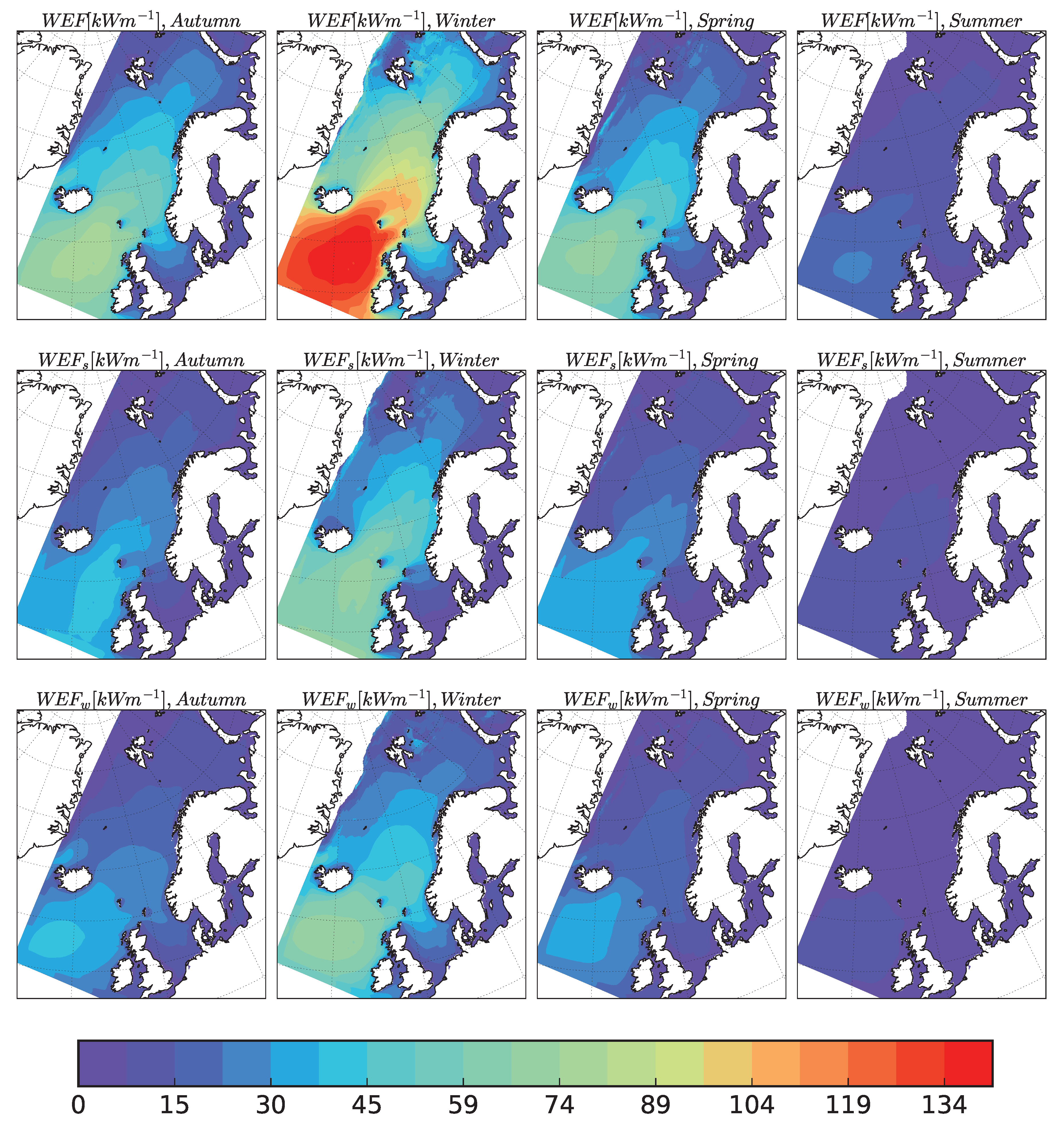
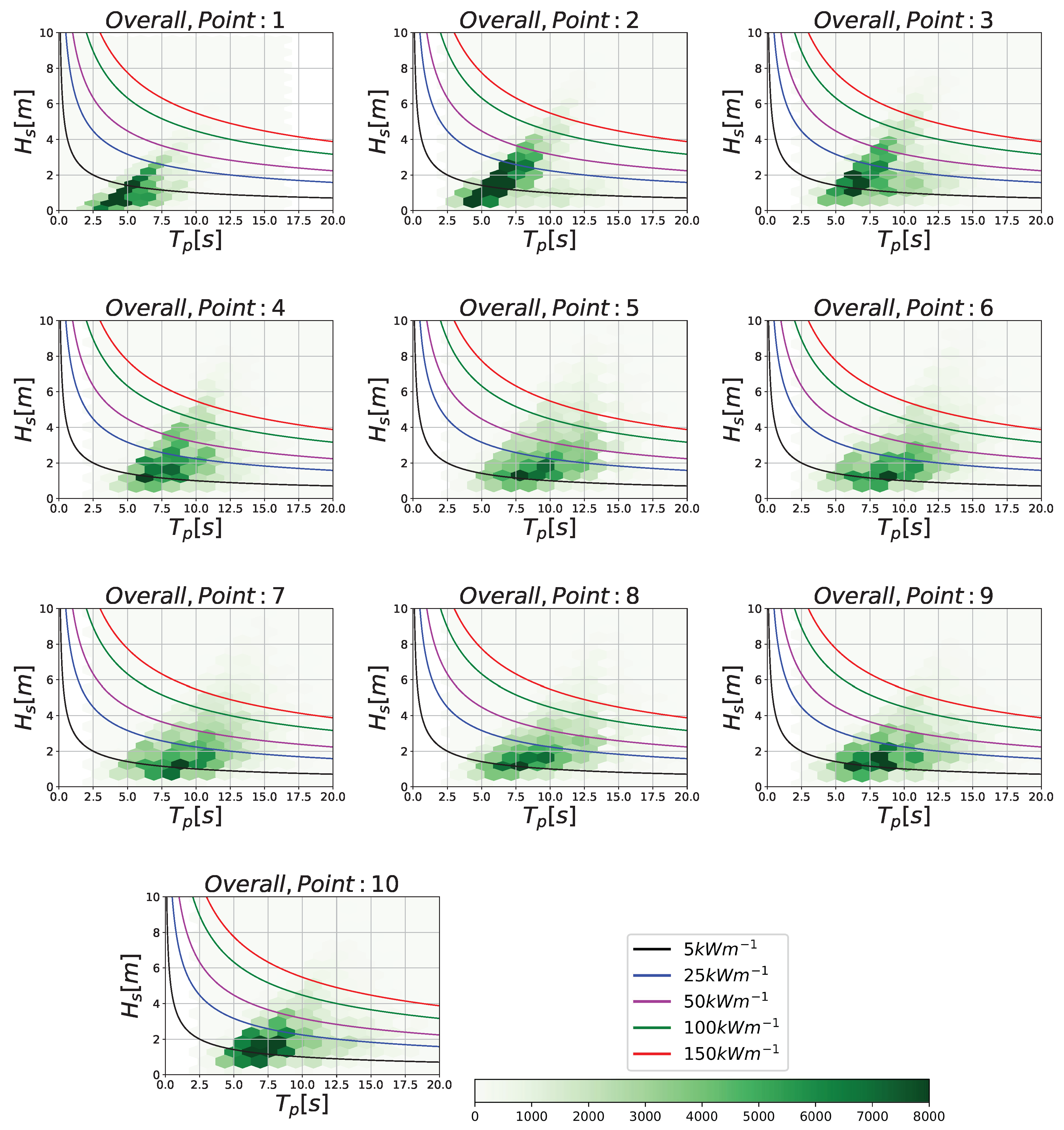
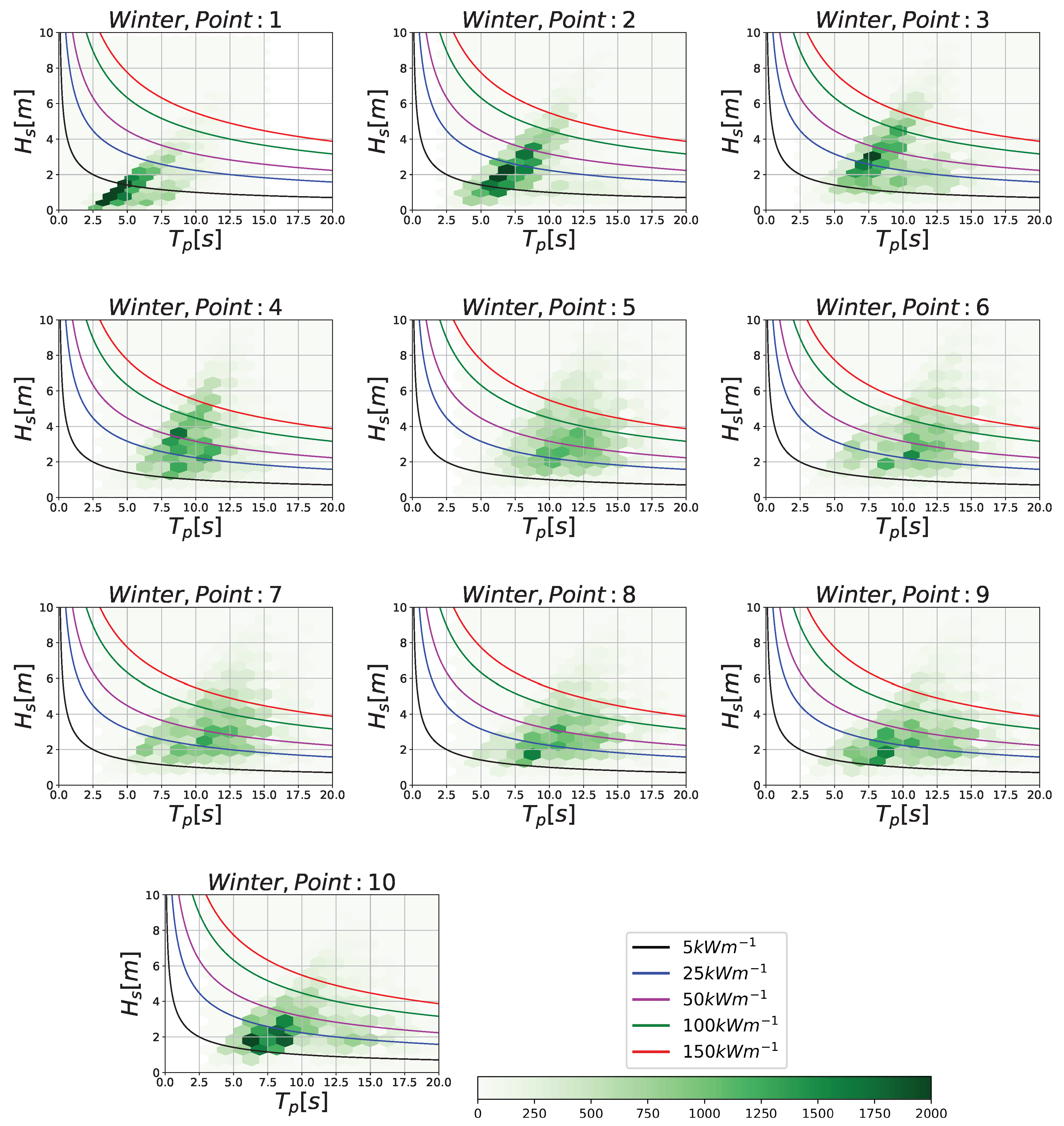
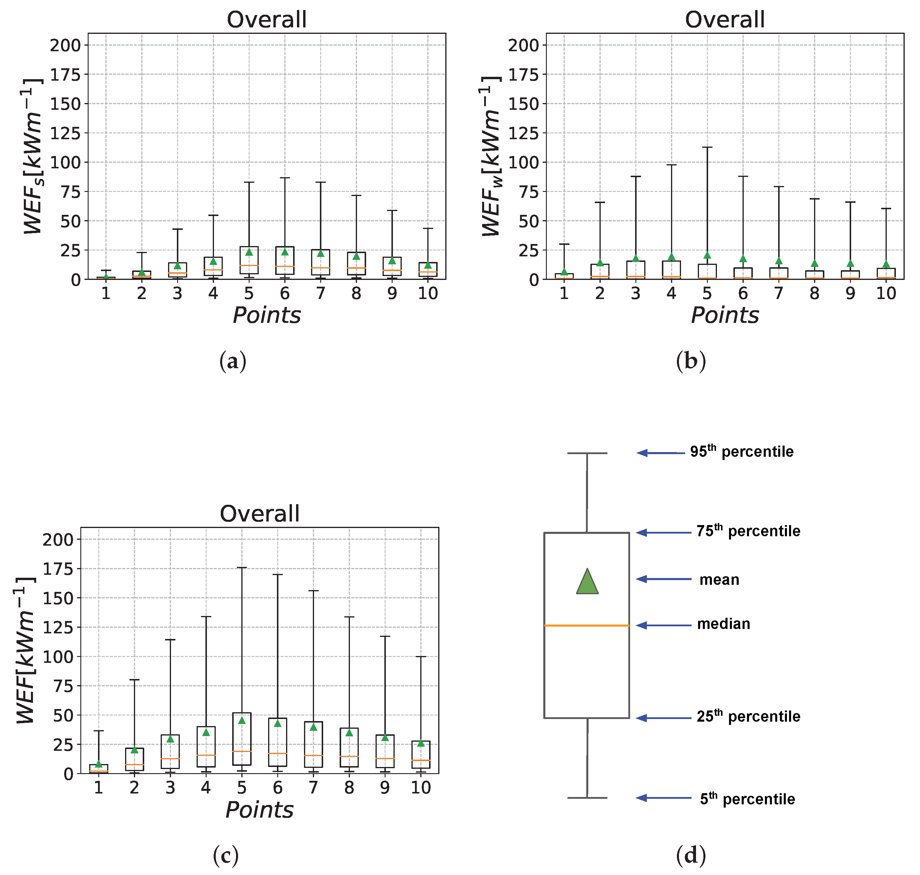
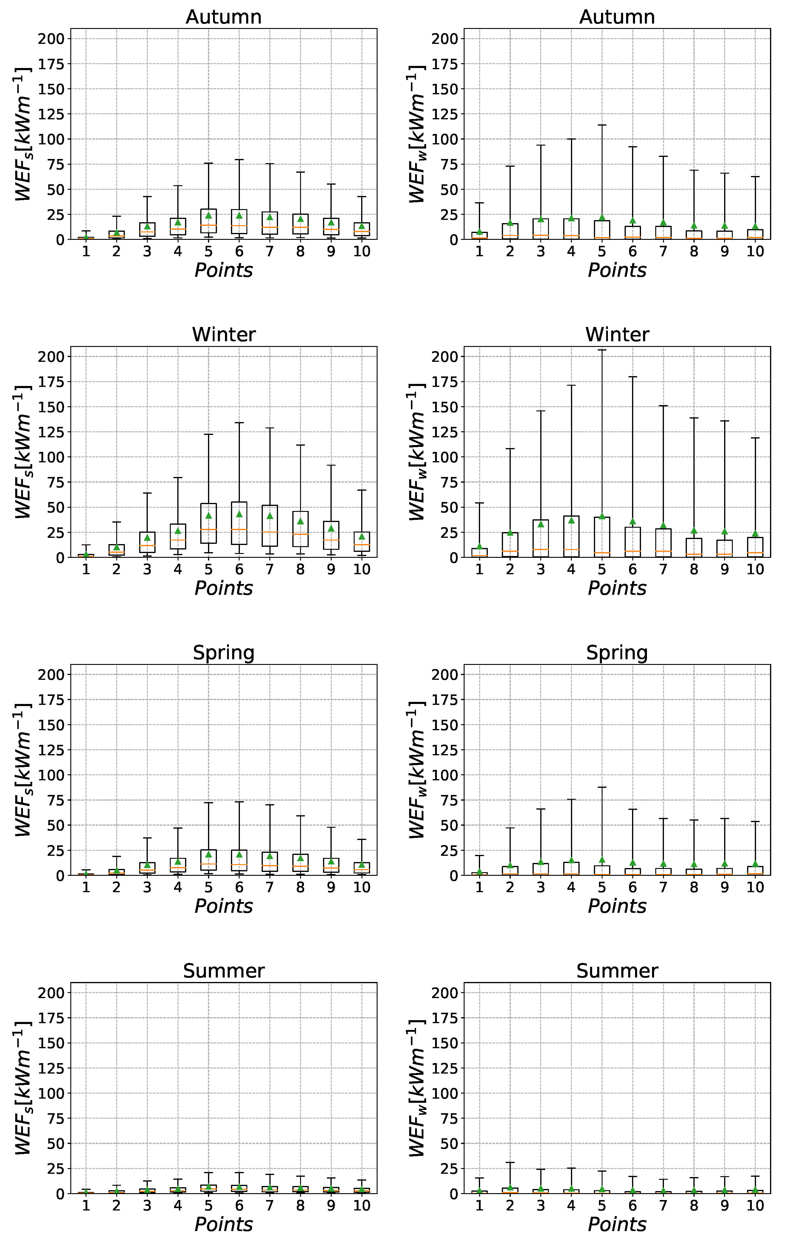
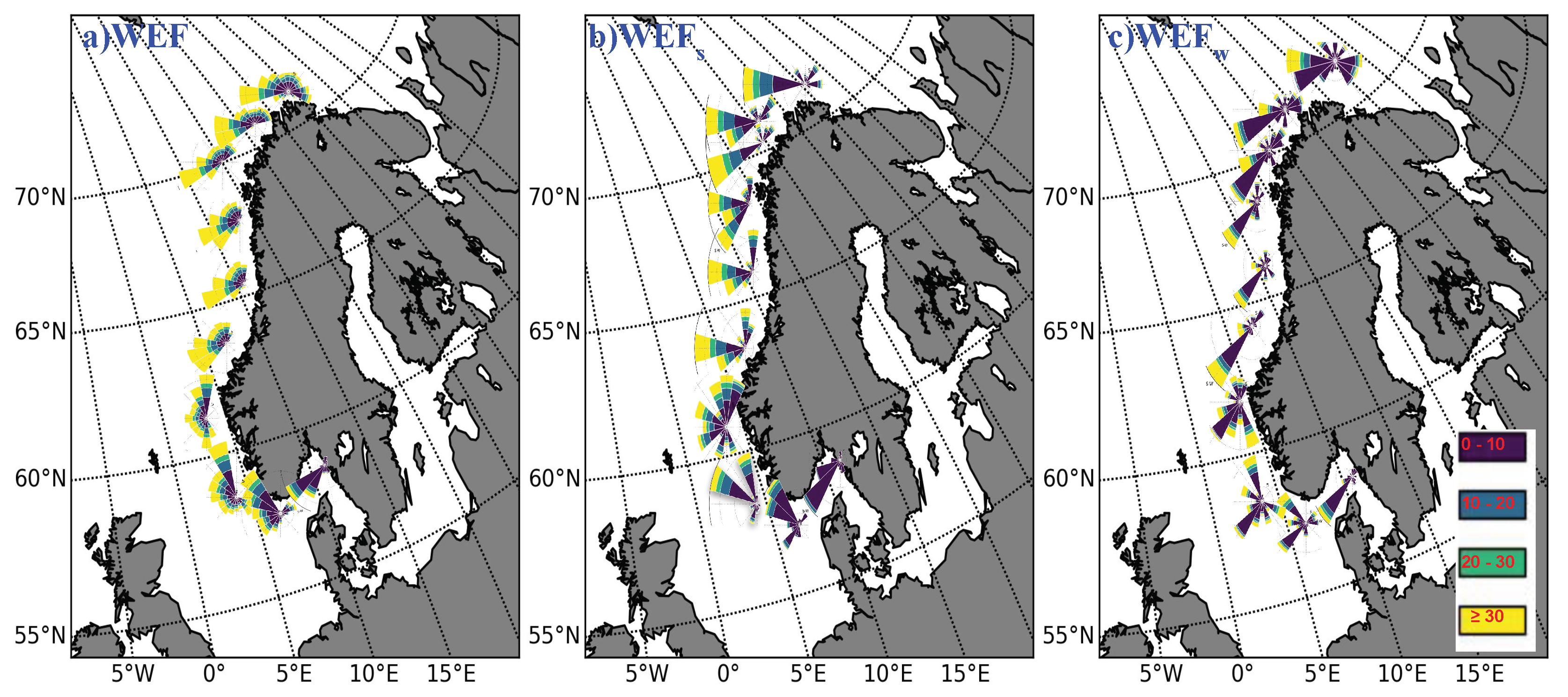
3.2. WEF along the Norwegian Coast

For a more detailed analysis of the coastal WEF, we investigated the wave energy fluxes induced by either swell or wind sea, in the 10 selected points. In general, WEF increased during the period from July to January while it decreased from February to July (

Table 1. Average monthly $WEF$ (kW m${}^{-1}$) for the 10 selected points.

Point	Jan	Feb	Mar	Apr	May	Jun	Jul	Aug	Sep	Oct	Nov	Dec	Total
1	15.97	10.64	8.11	3.95	3.38	3.99	3.91	3.97	7.07	10.05	12.52	15.42	8.25
2	37.95	29.07	23.53	13.15	8.40	8.69	8.14	8.70	15.99	23.31	30.97	36.63	20.38
3	56.83	45.26	38.58	21.13	12.16	9.37	7.94	9.65	20.89	34.57	45.16	55.10	29.72
4	68.80	54.98	46.52	26.11	14.60	10.68	8.64	10.37	23.85	40.07	52.03	65.70	35.20
5	89.75	79.54	63.32	33.03	16.69	12.88	10.42	12.37	31.00	48.61	62.31	86.15	45.51
6	85.95	79.07	59.67	30.16	14.65	11.55	8.97	10.92	28.67	45.75	58.73	81.40	42.96
7	80.41	74.88	56.41	27.23	12.98	10.13	7.97	9.90	25.98	42.80	54.43	74.90	39.83
8	68.06	66.05	50.39	24.71	13.00	10.41	7.88	9.67	22.24	39.17	46.26	62.46	35.02
9	58.22	58.58	45.27	21.99	12.10	9.79	7.26	9.09	19.78	35.36	39.83	53.84	30.92
10	47.29	48.30	37.33	19.44	11.39	9.24	6.97	8.92	17.67	30.85	33.76	43.71	26.24

). January and July were characterized by the highest and lowest WEF, respectively, while higher WEF values were observed at Points 4–7. The maximum monthly WEF was found for Point 5 in January, and it was equal to 89.8 kW m${}^{-1}$. Point 5 was also characterized by the maximum average annual WEF (45.5 kW m${}^{-1}$). The second highest WEF value was observed north of Point 5, at Point 6 where the average annual WEF was 43 kW m${}^{-1}$ and the monthly average for January was 86 kW m${}^{-1}$. For Northern Points 7–10, the average annual WEF values reduced from 39.8 to 26.2 kW m${}^{-1}$ and for the average monthly WEF for January from 80.4 to 47.3 kW m${}^{-1}$. South of Point 5 (Points 1–4), we also observed a reduction of annual and monthly WEF from Point 4 to Point 1. The average annual and monthly WEF values for January reduced from 35.2 to 8.3 kW m${}^{-1}$ and from 68.8 to 16 kW m${}^{-1}$, respectively. The previous results illustrate that the monthly WEF for January was about 2 times higher than the annual average WEF.

In order to further investigate the contribution of wind sea and swell on WEF, we plotted the $H_s$-$T_p$ diagrams for Points 1–10 considering all seasons of the 59-year period (Figure 6). In the most sheltered location from the open-sea conditions (Point 1), the majority of WEF values were below 25 kW m${}^{-1}$ with 2.5 s < $T_p$ < 9 s and 0 m < $H_s<3$ m. At Points 2–4, most WEF values were below 100 kW m${}^{-1}$ with 3 s < $T_p<11$ s and 0.5 m < $H_s<5$ m. Points 5–8 showed that most $WEF$ < 100 kW m${}^{-1}$ with 1 m <$H_s<4$ m but a higher $T_p$: 5–13 s. At Points 9–10, the WEF values were lower than 50 kW m${}^{-1}$ with 3 s < $T_p<12.5$ s and 0.5 m < $H_s<4$ m.

During winter, $H_s$ and $T_p$ were higher than the overall averaged values, leading to higher WEF (Figure 7). More specifically, for Point 1, most WEF values were two times higher than the overall, reaching 50 kW m${}^{-1}$ with 2.5 s < $T_p<9$ s and $H_s<4$ m. Even though the $T_p$ range was the same, the $H_s$ range increased by 1 m during winter. Most WEF values at Points 2–3 had a range 5 kW m${}^{-1}$ < $WEF$ < 50 kW m${}^{-1}$ with 1 m < $H_s<5$ m and 5 s < $T_p<10$ s. Point 4 was characterized by 5 kW m${}^{-1}$ < $WEF$ < 100 kW m${}^{-1}$ with 1.5 m < $H_s<5$ m and a slighter higher peak period 5 s < $T_p<11$ s due to its exposure to the Norwegian Sea. Point 5–10 had 5 kW m${}^{-1}$ < $WEF$ < 100 kW m${}^{-1}$ with 1.5 m < $H_s<5$ m and 5 s < $T_p<15$ s. Compared to the North Sea and the Barents Sea, the combination of high $H_s$ and $T_p$ in the Norwegian Sea (5–9) led to much higher values of $WEF$.

Table 2. Average monthly $WE{F}_s$ (kW m${}^{-1}$) for the 10 selected points.

Point	Jan	Feb	Mar	Apr	May	Jun	Jul	Aug	Sep	Oct	Nov	Dec	Total
1	3.19	2.43	1.92	1.05	0.90	1.04	1.03	1.10	1.45	2.17	2.70	3.01	1.83
2	10.66	9.15	7.51	4.60	2.84	2.39	2.09	2.50	4.69	6.68	9.15	10.71	6.08
3	20.02	17.75	15.65	9.75	5.55	3.89	3.39	4.12	8.58	12.96	17.35	20.75	11.65
4	27.00	23.88	21.14	12.82	7.22	5.00	4.27	5.08	11.05	17.72	22.55	27.80	15.46
5	43.69	39.62	33.03	19.21	10.35	7.55	6.27	7.26	15.85	24.31	31.43	41.31	23.32
6	45.14	41.03	33.75	18.57	9.48	7.31	5.85	6.86	15.83	24.43	31.03	42.41	23.47
7	43.32	40.45	31.79	16.99	8.63	6.60	5.17	6.37	15.09	22.57	28.87	40.05	22.16
8	37.66	35.18	27.92	15.20	8.02	6.17	4.91	6.02	13.72	21.39	26.31	35.02	19.79
9	29.80	28.51	22.45	12.31	6.63	5.27	4.26	5.30	11.49	17.76	21.18	27.83	16.07
10	21.47	20.69	16.52	9.62	5.42	4.63	3.58	4.60	9.28	14.48	16.13	20.31	12.23

and

Table 3. Average monthly $WE{F}_w$ (kW m${}^{-1}$) for the 10 selected points.

Point	Jan	Feb	Mar	Apr	May	Jun	Jul	Aug	Sep	Oct	Nov	Dec	Total
1	12.67	8.11	6.14	2.88	2.45	2.92	2.86	2.84	5.59	7.82	9.74	12.32	6.36
2	27.36	19.90	15.99	8.47	5.50	6.26	6.03	6.18	11.28	16.59	21.76	25.94	14.27
3	36.93	27.48	22.79	10.99	6.39	5.38	4.45	5.41	12.13	21.41	27.49	34.25	17.93
4	41.70	30.93	25.16	12.83	7.16	5.54	4.26	5.12	12.59	22.01	29.09	37.47	19.49
5	43.27	37.30	28.21	12.70	5.80	4.93	3.78	4.71	14.28	22.92	28.89	42.23	20.75
6	37.38	34.76	23.54	10.36	4.63	3.84	2.80	3.68	11.91	19.66	25.40	35.73	17.81
7	33.43	30.90	21.87	8.97	3.79	3.08	2.47	3.13	9.80	18.39	22.95	31.51	15.86
8	27.49	28.33	20.25	8.60	4.55	3.88	2.69	3.28	7.64	16.36	17.83	24.89	13.82
9	26.23	27.81	20.99	8.90	5.13	4.24	2.77	3.48	7.56	16.47	16.93	23.93	13.70
10	24.23	25.87	19.48	9.29	5.74	4.37	3.24	4.09	7.79	15.41	16.25	21.78	13.13

present the average monthly and annual $WE{F}_s$ and $WE{F}_w$, respectively. Regarding $WE{F}_w$, we observed that the maximum was located at Point 5 with an average annual value at 20.8 kW m${}^{-1}$. The second highest $WE{F}_w$ was at Point 4 with 19.5 kW m${}^{-1}$. For points north (6–10) and south (1–4) of Point 5, the $WE{F}_w$ decreased from 17.8 to 13.1 kW m${}^{-1}$ and from 19.5 to 6.4 kW m${}^{-1}$, respectively. Similarly with the total WEF, the maximum monthly values were observed during the winter months, where January had the highest $WE{F}_w$ at Point 5, equal to 43.3 kW m${}^{-1}$, followed by 41.7 kW m${}^{-1}$ at Point 4. On the other hand, $WE{F}_s$ showed the maximum average annual value of 23.5 kW m${}^{-1}$ at Point 6, which was slightly higher (by 0.2 kW m${}^{-1}$) at Point 5. As observed for $WE{F}_w$, the $WE{F}_s$ values decreased towards Point 1, where swell was nearly absent ($WE{F}_s$ < 2 kW m${}^{-1}$). For Points 7–10, $WE{F}_s$ was also decreasing from 22.2 kW m${}^{-1}$ to 12.2 kW m${}^{-1}$. January was the month with the highest $WE{F}_s$, with 45.1 kW m${}^{-1}$ at Point 6 followed by 43.7 kW m${}^{-1}$ at Point 5.

Figure 8 presents the overall (59-year period) boxplots for total $WEF$, $WE{F}_w$, and $WE{F}_s$ for the 10 selected points. The definition of boxplot used in this study is given in Figure 8d i.e., the green triangle: the mean, the horizontal orange line: 50th percentile or median, the lower quantile: 25th percentile, the upper quantile: 75th percentile, the maximum: 95th percentile and the minimum: 5th percentile. The maximum $WEF$ in the North Sea (Points 1–4) was greater than 30 kW m${}^{-1}$, $WE{F}_s>10$ kW m${}^{-1}$ and $WE{F}_w>30$ kW m${}^{-1}$. The maximum $WEF$ in the Norwegian Sea (Points 5-9) exceeded 120 kW m${}^{-1}$ with $WE{F}_s>50$ kW m${}^{-1}$ and $WE{F}_w>60$ kW m${}^{-1}$. The maximum $WEF$ was observed at Point 5, slightly exceeding 175 kW m${}^{-1}$. At the same location, $WE{F}_s$ and $WE{F}_w$ were above 75 kW m${}^{-1}$ and 100 kW m${}^{-1}$, respectively.

$WE{F}_w$ showed higher variability compare to $WE{F}_s$ (Figure 8). It is noteworthy that the mean values for $WE{F}_w$ were higher than the 75th percentile and that its median was close to zero (dominated by low wind/calm conditions). In addition, the maximum $WE{F}_w$ exceeded the maximum $WE{F}_s$ at all points. This shows that the extreme events induced higher variability to $WE{F}_w$ than $WE{F}_s$. On the other hand, the mean $WE{F}_s$ was below the 75th percentile and closer to the median, showing that the distribution of $WE{F}_s$ was more symmetric than $WE{F}_w$’s distribution. Additionally, higher median values for $WE{F}_s$ were detected, showing the presence of swell waves along the coast most of the time.

The seasonal boxplots (Figure 9) of $WE{F}_s$ and $WE{F}_w$ for the 10 selected points show that the highest WEF values were observed during winter followed by autumn, spring, and summer (the lowest values). In more detail, during winter, the maximum $WE{F}_s$ was greater than 100 kW m${}^{-1}$ at Points 5–8, while the maximum $WE{F}_w$ was higher than 150 kW m${}^{-1}$ at Points 4–6. During autumn and spring, the maximum $WE{F}_s$ were below 85 kW m${}^{-1}$ and the maximum $WE{F}_w<125$ kW m${}^{-1}$. During summer, the maximum $WE{F}_s$ and $WE{F}_w$ were lower than 25 kW m${}^{-1}$ and 30 kW m${}^{-1}$, respectively. Regarding the seasonal variability of WEF components, the winter season showed the highest variability followed by autumn and spring. During summer, there was nearly no variability due to the relative low WEF values. During all seasons, wind-sea-induced WEF had higher variability compared to $WE{F}_s$.

The direction of $WE{F}_w$, $WE{F}_s$, and total WEF was analyzed using the corresponding roses along the coast, which are plotted in Figure 10. The roses illustrated how the WEF direction was distributed at a specific location. For wind sea conditions and Points 1 and 5–10, the dominant direction was southwest, which was parallel to the coast. For Points 2–4, we detected a dominant direction from southwest with a secondary direction from southeast and northwest. For $WE{F}_s$, the main direction was west/southwest for Points 5–10, north/northwest for Points 2–4, and southwest for Point 1. The total WEF followed the dominant directions of $WE{F}_w$ and $WE{F}_s$. More specifically, the main direction was southwest at Points 1 and 5–10 and north/northwest for Points 2–4.

4. Discussion

The differences in wave climate observed in the Nordic Seas significantly affect the coastal wave conditions of Norway. The application of a high resolution wind-wave hindcast, such as NORA10, facilitates a high-quality representation of wave conditions both in regional and coastal scales.

Our regional analysis showed that both swell and wind sea waves transfer a significant amount of wave energy to the Norwegian coast. The results indicate higher swell than wind sea in the Norwegian Sea, while swell is less pronounced in the North and Barents Seas. These results are in agreement with the study of Semedo et al. [47]. Hence, the Norwegian Sea is characterized by the highest WEF, since WEF is most strongly dependent on significant wave height (quadratic relation) and wave period (linear relation). This is attributed to the fact that the Norwegian Sea is exposed to high ocean waves originating from the Northeast Atlantic Ocean. The swell waves dominate the wave climate of the Norwegian Sea, which is also noted with a high $WE{F}_s$. Moreover, a high $WE{F}_w$ is also observed in the Norwegian Sea, due to the strong local winds in the area. On the other hand, the $WE{F}_s$ is lower compared to $WE{F}_w$ in the North Sea due to sheltering by the British Isles. The highest values of WEF in the North Sea are observed in its northern region due to the exposure to swell propagated through the Norwegian Sea, which is also indicated in the study of Lavidas and Polinder [48]. Even though they applied different methods (e.g., the spectral wave model, model set-up, estimation of $T_e$, and time period), the WEF estimations are in agreement with our results (< 20 kW m${}^{-1}$ in the southern parts of the North Sea). Similarly to the North Sea, the Barents Sea is characterized by weaker $WE{F}_s$ compared to the Norwegian Sea, since the swell waves reaching the northern part of Norway propagate over longer distances and are partly dissipated. In addition, due to lower winds in the Barents Sea compared to the North Sea, a slightly lower $WE{F}_w$ is observed.

In order to thoroughly investigate the coastal wave climate, we identified areas along the coast where wind sea or swell is the dominant source of wave energy. As it was also indicated in the regional analysis, wind sea is dominant in areas located in the North Sea, i.e., Points 1–4 and in the northernmost region (Barents Sea), Point 10 (Figure 1). Points 1–4 are less exposed to swell conditions due to sheltering by the British Isles. Moreover, Point 1 is characterized by the lowest WEF, $WE{F}_s$, and $WE{F}_w$ due to sheltering and limited fetches. Swell waves reaching the coast of Norway are mostly generated by cyclones in the Northeast Atlantic Ocean, as also discussed by Varlas et al. [43]. Our analysis shows that the swell waves are dominant at Points 5–9 located in the Norwegian Sea, because these areas are exposed directly to open ocean.

As far as the seasonal variability is concerned, winter is characterized by the maximum WEF, and summer by the minimum. The monthly distribution of $WE{F}_w$ and $WE{F}_s$ are similar to the total WEF, with maximum in January at the central points and minimum in July at the enclosed Point 1. In comparison with $WE{F}_w$, $WE{F}_s$ is lower at Points 1–4 and 10, but higher at Points 5–9. Moreover, it is noteworthy that $WE{F}_w$ presents higher variability than $WE{F}_s$, as illustrated in the boxplots. The wind sea conditions are often characterized by high variations following the sharply changing weather conditions and mesoscale coastal phenomena such as the low level coastal jets [49,50]. In addition to high $WE{F}_w$ during cold months, when low pressure systems generate high swell waves at open sea, the Norwegian coasts receive large amounts of wave energy. This highlights the importance of the wave energy flux analysis individually for wind sea and swell, as it is difficult to unveil the source of WEF only considering the total WEF. Moreover, as illustrated on the boxplots, winter is characterized by increased WEF variability and the highest peaks for both $WE{F}_s$ and $WE{F}_w$.

Along the Norwegian coastline, we observe significant spatial differences in wave climate leading to high spatial variations of WEF. Point 1 has the lowest wave heights and periods leading to the minimum WEF during all the months of the year. This is attributed to the fact that it is located in a semi-closed area, where less wave energy originated from the North Sea is transported. On the other hand, Points 5–6 have the highest WEF due to their exposure to open sea. As is also illustrated on the $H_s$-$T_p$ diagrams of peak spectral wave period and significant wave height (Figure 6 and Figure 7), most values at Point 1 are lower than those at Points 5–6. Point 1 is dominated by waves with $T_p<10$ s, while Points 5–6 are exposed to much longer waves, up to 15 s.

Finally, the WAM model is designed for ocean scale applications, and NORA10 spatial resolution can be considered as a high for climate studies, given the wide coverage area. In our study, the selected points are located ca. 30–70 km from the coast in deep water areas, where the WAM model is suitable and the estimation of WEF based on Equation (2) is valid (deep water). However, for wave energy assessment nearshore and within the fjord systems, higher spatial resolution is needed, and wave models for coastal applications such as SWAN [51] are more suitable. It was shown in Christakos et al. [52] that the SWAN model with a high spatial resolution (250 m) performs well for the coastal and fjord wave conditions. They also found that the use of a finer grid improves the quality of wave predictions in most fjord locations.

5. Conclusions

This study presents a characterization of wave energy flux in the Nordic Seas with a focus on the Norwegian coastline. The WEF, $WE{F}_w$, and $WE{F}_s$ are derived using the NORA10 hindcast data for the period 1958–2017. The highest coastal wave energy flux is observed in the Norwegian Sea. The majority of areas with dominant swell conditions (i.e., in the Norwegian Sea) are characterized by the highest wave energy flux. The maximum values of WEF in the North Sea are denoted in its northern parts in the intersection with the Norwegian Sea. In contrast to the Norwegian Sea, areas located in the North Sea and the Barents Sea show that wind sea is contributing more than swell to the total wave energy flux. A high seasonal and spatial variability of wave energy flux along the coast is observed. Even though the point locations are close to each other, significant differences have been observed due to sheltering effects and limited fetches. More specifically, in areas where swell conditions are dominant, we observe the highest WEF along the coast such as Points 5–6 (Figure 1). These areas are characterized by both strong swell and wind sea conditions. Regarding the seasonal variability, winter is characterized by the maximum WEF, and summer by the minimum, as expected. The swell waves are associated with higher WEF than those of the wind sea; WEF exceeds 35 kW m${}^{-1}$ (Table 1) at the central coast of Norway where swell is pronounced. This is attributed to the propagation of significant amounts of swell-induced wave energy from the Northeastern Atlantic Ocean. The results of our analysis indicate that WEF is affected by cyclonic activity especially at the central parts of the Norwegian coast. $WE{F}_w$ shows the highest variability and a less symmetric distribution with its median close to zero. On the other hand, $WE{F}_s$ shows less variability with its median closer to mean, indicating the existence of swell energy most of the time, especially at Points 4–10. Therefore, during low-wind events, the reduced wind energy production could be compensated by wave energy transferred by swell waves originating from the open ocean. This analysis can potentially be a valuable tool for choosing the proper area for wave energy installations along the Norwegian coast.

References

1. European Commission. A Clean Planet for All—A European Long-Term Strategic Vision for a Prosperous, Modern, Competitive and Climate Neutral Economy; Technical Report; European Commission: Brussels, Belgium, 2018. [Google Scholar]
2. Twidell, J.; Weir, T. Renewable Energy Resources; Routledge: London, UK, 2015. [Google Scholar] [CrossRef]
3. Borthwick, A.G.L. Marine Renewable Energy Seascape. Engineering 2016, 2, 69–78. [Google Scholar] [CrossRef] [Green Version]
4. Grabbe, M.; Lalander, E.; Lundin, S.; Leijon, M. A review of the tidal current energy resource in Norway. Renew. Sustain. Energy Rev. 2009, 13, 1898–1909. [Google Scholar] [CrossRef] [Green Version]
5. Astariz, S.; Iglesias, G. The economics of wave energy: A review. Renew. Sustain. Energy Rev. 2015, 45, 397–408. [Google Scholar] [CrossRef]
6. Magagna, D.; Uihlein, A. Ocean energy development in Europe: Current status and future perspectives. Int. J. Mar. Energy 2015, 11, 84–104. [Google Scholar] [CrossRef]
7. Pérez-Collazo, C.; Greaves, D.; Iglesias, G. A review of combined wave and offshore wind energy. Renew. Sustain. Energy Rev. 2015, 42, 141–153. [Google Scholar] [CrossRef] [Green Version]
8. Uihlein, A.; Magagna, D. Wave and tidal current energy—A review of the current state of research beyond technology. Renew. Sustain. Energy Rev. 2016, 58, 1070–1081. [Google Scholar] [CrossRef]
9. Chatzigiannakou, M.; Temiz, I.; Leijon, M. Offshore Deployments of Wave Energy Converters by Seabased Industry AB. J. Mar. Sci. Eng. 2017, 5, 15. [Google Scholar] [CrossRef]
10. Wang, Z. New wave power. Nature 2017, 542, 159–160. [Google Scholar] [CrossRef]
11. Aderinto, T.; Li, H. Ocean Wave Energy Converters: Status and Challenges. Energies 2018, 11, 1250. [Google Scholar] [CrossRef] [Green Version]
12. Lavidas, G. Energy and socio-economic benefits from the development of wave energy in Greece. Renew. Energy 2019, 132, 1290–1300. [Google Scholar] [CrossRef]
13. Reguero, B.G.; Losada, I.J.; Méndez, F.J. A recent increase in global wave power as a consequence of oceanic warming. Nat. Commun. 2019, 10, 205. [Google Scholar] [CrossRef] [PubMed] [Green Version]
14. Clément, A.; McCullen, P.; Falcão, A.; Fiorentino, A.; Gardner, F.; Hammarlund, K.; Lemonis, G.; Lewis, T.; Nielsen, K.; Petroncini, S.; et al. Wave energy in Europe: Current status and perspectives. Renew. Sustain. Energy Rev. 2002, 6, 405–431. [Google Scholar] [CrossRef]
15. Gunn, K.; Stock-Williams, C. Quantifying the global wave power resource. Renew. Energy 2012, 44, 296–304. [Google Scholar] [CrossRef]
16. Falnes, J. Research and development in ocean-wave energy in Norway. In Proceedings of the International Symposium on Ocean Energy Development, Muroran, Hokkaido, Japan, 26–27 August 1993; pp. 27–39. [Google Scholar]
17. Kalogeri, C.; Galanis, G.; Spyrou, C.; Diamantis, D.; Baladima, F.; Koukoula, M.; Kallos, G. Assessing the European offshore wind and wave energy resource for combined exploitation. Renew. Energy 2017, 101, 244–264. [Google Scholar] [CrossRef]
18. Saha, P.; Idsø, J. New hydropower development in Norway: Municipalities’ attitude, involvement and perceived barriers. Renew. Sustain. Energy Rev. 2016, 61, 235–244. [Google Scholar] [CrossRef]
19. Cheliotis, I.; Varlas, G.; Christakos, K. The Impact of Cyclone Xaver on Hydropower Potential in Norway. In Perspectives on Atmospheric Sciences; Springer International Publishing: Cham, Switzerland, 2017; pp. 175–181. [Google Scholar]
20. Strbac, G.; Hatziargyriou, N.; Lopes, J.P.; Moreira, C.; Dimeas, A.; Papadaskalopoulos, D. Microgrids: Enhancing the Resilience of the European Megagrid. IEEE Power Energy Mag. 2015, 13, 35–43. [Google Scholar] [CrossRef] [Green Version]
21. Rusu, E.; Onea, F. A review of the technologies for wave energy extraction. Clean Energy 2018, 1. [Google Scholar] [CrossRef] [Green Version]
22. Katsafados, P.; Papadopoulos, A.; Korres, G.; Varlas, G. A fully coupled atmosphere–ocean wave modeling system for the Mediterranean Sea: Interactions and sensitivity to the resolved scales and mechanisms. Geosci. Model Dev. 2016, 9, 161–173. [Google Scholar] [CrossRef] [Green Version]
23. Varlas, G.; Katsafados, P.; Papadopoulos, A.; Korres, G. Implementation of a two-way coupled atmosphere-ocean wave modeling system for assessing air-sea interaction over the Mediterranean Sea. Atmos. Res. 2018, 208, 201–217. [Google Scholar] [CrossRef]
24. Katsafados, P.; Varlas, G.; Papadopoulos, A.; Spyrou, C.; Korres, G. Assessing the Implicit Rain Impact on Sea State During Hurricane Sandy (2012). Geophys. Res. Lett. 2018. [Google Scholar] [CrossRef]
25. Zheng, C.; Shao, L.; Shi, W.; Su, Q.; Lin, G.; Li, X.; Chen, X. An assessment of global ocean wave energy resources over the last 45 a. Acta Oceanol. Sin. 2014, 33, 92–101. [Google Scholar] [CrossRef]
26. Cornett, A. A Global Wave Energy Resource Assessment. In Proceedings of the Eighteenth International Offshore and Polar Engineering Conference, Vancouver, BC, Canada, 6–11 July 2008; Volume 50. [Google Scholar]
27. The WAVEWATCHIII® Development Group. User Manual and System Documentation of WAVEWATCH III® Version 5.16; Technical Report 329; NOAA/NWS/NCEP/MMAB: College Park, MD, USA, 2016. [Google Scholar]
28. Reistad, M.; Breivik, Ø.; Haakenstad, H.; Aarnes, O.J.; Furevik, B.R.; Bidlot, J.R. A high-resolution hindcast of wind and waves for the North Sea, the Norwegian Sea, and the Barents Sea. J. Geophys. Res. Oceans 2011, 116. [Google Scholar] [CrossRef] [Green Version]
29. Furevik, B.R.; Haakenstad, H. Near-surface marine wind profiles from rawinsonde and NORA10 hindcast. J. Geophys. Res. Atmos. 2012, 117. [Google Scholar] [CrossRef]
30. Uppala, S.; Kallberg, P.; Simmons, A.J.; Andrae, U.; Da Costa Bechtold, V.; Fiorino, M.; Gibson, J.K.; Haseler, J.; Hernandez-Carrascal, A.; Kelly, G.A.; et al. The Era-40 Re-analysis. Q. J. R. Meteorol. Soc. 2005, 131, 2961–3012. [Google Scholar] [CrossRef]
31. Undén, P.; Rontu, L.; Järvinen, H.; Lynch, P.; Calvo-Sanchez, J.; Cats, G.; Cuxart, J.; Eerola, K.; Fortelius, C.; García-Moya, J. HIRLAM-5 Scientific Documentation; Technical Report; Sveriges Meteorologiska Och Hydrologiska Institut: Norrköping, Sweden, 2002. [Google Scholar]
32. ECMWF. Part VII: ECMWF Wave Model. In IFS Documentation CY45R1; Number 7 in IFS Documentation; ECMWF: Reading, UK, 2018; Chapter 10; p. 70. [Google Scholar]
33. Aarnes, O.J.; Breivik, Ø.; Reistad, M. Wave Extremes in the Northeast Atlantic. J. Clim. 2012, 25, 1529–1543. [Google Scholar] [CrossRef] [Green Version]
34. Iglesias, G.; López, M.; Carballo, R.; Castro, A.; Fraguela, J.; Frigaard, P. Wave energy potential in Galicia (NW Spain). Renew. Energy 2009, 34, 2323–2333. [Google Scholar] [CrossRef]
35. Herbich, J.B. Handbook of Coastal Engineering, 1st ed.; McGraw-Hill Professional: New York, NY, USA, 2000. [Google Scholar]
36. Falnes, J. A review of wave-energy extraction. Mar. Struct. 2007, 20, 185–201. [Google Scholar] [CrossRef]
37. Izadparast, A.H.; Niedzwecki, J.M. Estimating the potential of ocean wave power resources. Ocean Eng. 2011, 38, 177–185. [Google Scholar] [CrossRef]
38. Bento, A.R.; Martinho, P.; Guedes Soares, C. Wave energy assessement for Northern Spain from a 33-year hindcast. Renew. Energy 2018, 127, 322–333. [Google Scholar] [CrossRef]
39. Akpınar, A.; Jafali, H.; Rusu, E. Temporal Variation of the Wave Energy Flux in Hotspot Areas of the Black Sea. Sustainability 2019, 11, 562. [Google Scholar] [CrossRef] [Green Version]
40. Holthuijsen, L. Waves in Oceanic and Coastal Waters; Cambridge University Press: Cambridge, UK, 2007. [Google Scholar] [CrossRef]
41. Cahill, B.; Lewis, T. Wave period ratios and the calculation of wave power. In Proceedings of the 2nd Marine Energy Technology Symposium METS2014, Seattle, WA, USA, 15–18 April 2014. [Google Scholar]
42. Santo, H.; Taylor, P.H.; Woollings, T.; Poulson, S. Decadal wave power variability in the North-East Atlantic and North Sea. Geophys. Res. Lett. 2015, 42, 4956–4963. [Google Scholar] [CrossRef]
43. Varlas, G.; Christakos, K.; Cheliotis, I.; Papadopoulos, A.; Steeneveld, G.J. Spatiotemporal variability of marine renewable energy resources in Norway. Energy Procedia 2017, 125, 180–189. [Google Scholar] [CrossRef]
44. Sasaki, W. Changes in wave energy resources around Japan. Geophys. Res. Lett. 2012, 39. [Google Scholar] [CrossRef]
45. Goddijn-Murphy, L.; Míguez, B.M.; McIlvenny, J.; Gleizon, P. Wave energy resource assessment with AltiKa satellite altimetry: A case study at a wave energy site. Geophys. Res. Lett. 2015, 42, 5452–5459. [Google Scholar] [CrossRef]
46. Boronowski, S.; Wild, P.; Rowe, A.; Cornelis van Kooten, G. Integration of wave power in Haida Gwaii. Renew. Energy 2010, 35, 2415–2421. [Google Scholar] [CrossRef]
47. Semedo, A.; Vettor, R.; Breivik, O.; Sterl, A.; Reistad, M.; Lima, D. The wind sea and swell waves climate in the Nordic seas. Ocean Dyn. 2014, 65. [Google Scholar] [CrossRef]
48. Lavidas, G.; Polinder, H. North Sea Wave Database (NSWD) and the Need for Reliable Resource Data: A 38 Year Database for Metocean and Wave Energy Assessments. Atmosphere 2019, 10, 551. [Google Scholar] [CrossRef] [Green Version]
49. Christakos, K.; Varlas, G.; Reuder, J.; Katsafados, P.; Papadopoulos, A. Analysis of a Low-level Coastal Jet off the Western Coast of Norway. Energy Procedia 2014, 53, 162–172. [Google Scholar] [CrossRef] [Green Version]
50. Christakos, K.; Cheliotis, I.; Varlas, G.; Steeneveld, G.J. Offshore Wind Energy Analysis of Cyclone Xaver over North Europe. Energy Procedia 2016, 94, 37–44. [Google Scholar] [CrossRef] [Green Version]
51. SWAN Team. Scientific and Technical Documentation SWAN Cycle III Version 41.31; Delft University of Technology: Delft, The Netherlands, 2019. [Google Scholar]
52. Christakos, K.; Furevik, B.R.; Aarnes, O.J.; Breivik, Ø.; Tuomi, L.; Byrkjedal, Ø. The importance of wind forcing in fjord wave modelling. Ocean Dyn. 2020, 70, 57–75. [Google Scholar] [CrossRef] [Green Version]
Figure 1. The 10 selected offshore points (red dots and numbers) along the Norwegian coastline. Areas dominated by wind sea ( W E F w ¯ > W E F s ¯ ) within blue-curve and areas dominated by swell ( W E F s ¯ > W E F w ¯ ) within green-curve. The dashed arrows show the direction of swell decay along the coast.
Atmosphere 11 00166 g001
Figure 2. The average H s , H s , s , H s , w , T p , T p , s , T p , w , W E F , W E F s , and W E F w for the NORA10 domain for the period 1958–2017.
Atmosphere 11 00166 g002
Figure 3. The average seasonal (autumn, winter, spring, and summer) H s , H s , s , and H s , w for the NORA10 domain for the period 1958–2017.
Atmosphere 11 00166 g003
Figure 4. The average seasonal (autumn, winter, spring, and summer) T p , T p , s , and T p , w for the NORA10 domain for the period 1958–2017.
Atmosphere 11 00166 g004
Figure 5. The average seasonal (autumn, winter, spring, and summer) W E F , W E F s , and W E F w for the NORA10 domain for the period 1958–2017.
Atmosphere 11 00166 g005
Figure 6. H s - T p diagram of peak wave period (s; x-axis) and total significant wave height (m; y-axis) during the 59-year period for Points 1–10. Colored areas and contours represent occurrence and WEF (kW m 1 ), respectively.
Atmosphere 11 00166 g006
Figure 7. H s - T p diagram of peak wave period (s; x-axis) and total significant wave height (m; y-axis) during the winter season for Points 1–10. Colored areas and contours represent occurrence and WEF (kW m 1 ), respectively.
Atmosphere 11 00166 g007
Figure 8. Boxplots based on the 59-year period for (a) swell-induced and (b) wind-sea-induced WEF as well as (c) total WEF (kW m 1 ) for the 10 selected offshore points (x-axis). (d) Definition of boxplot used in this study, where the whiskers are set at specific percentiles (5, 95) of the data.
Atmosphere 11 00166 g008
Figure 9. Seasonal boxplots for swell-induced (left) and wind-sea-induced (right) Wave Energy Flux (WEF) (kW m 1 ) for the 10 selected offshore points (x-axis).
Atmosphere 11 00166 g009
Figure 10. Roses of (a) total as well as (b) swell- and (c) wind-sea-induced WEF along the Norwegian coast. The colors illustrate the WEF intervals, purple: from 0 to 10 kW m 1 ; light blue: from 10 to 20 kW m 1 ; cyan: from 20 to 30 kW m 1 ; yellow: greater than 30 kW m 1 .
Atmosphere 11 00166 g010