Long-Term Variations of Air Quality Influenced by Surface Ozone in a Coastal Site in India: Association with Synoptic Meteorological Conditions with Model Simulations


Abstract
:1. Introduction
2. Experimental Method
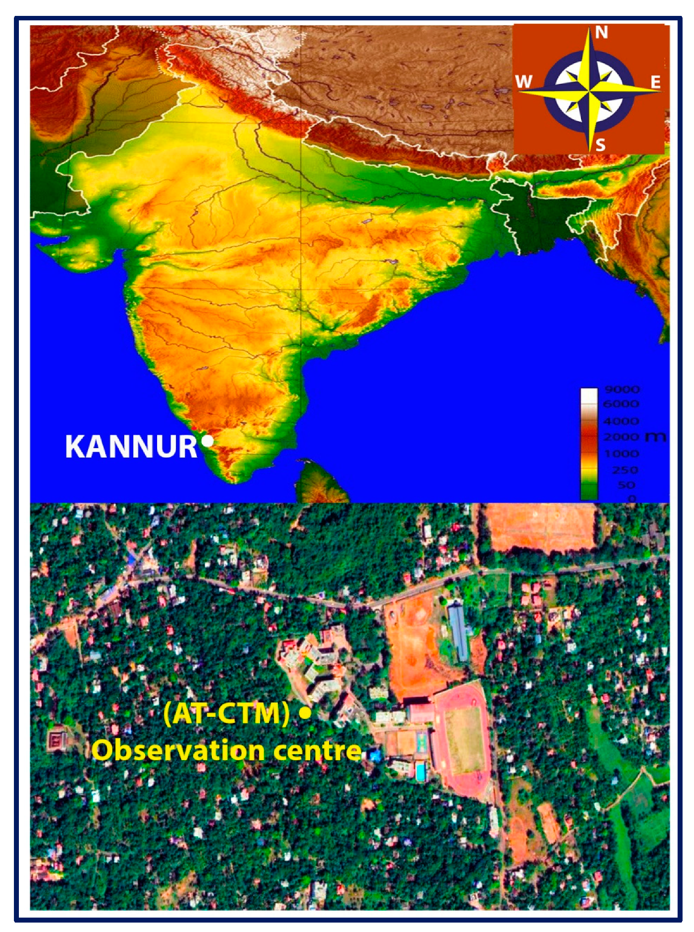
2.1. Observational Site and Measurement Techniques
2.2. Artificial Neural Network
3. Results and Discussions
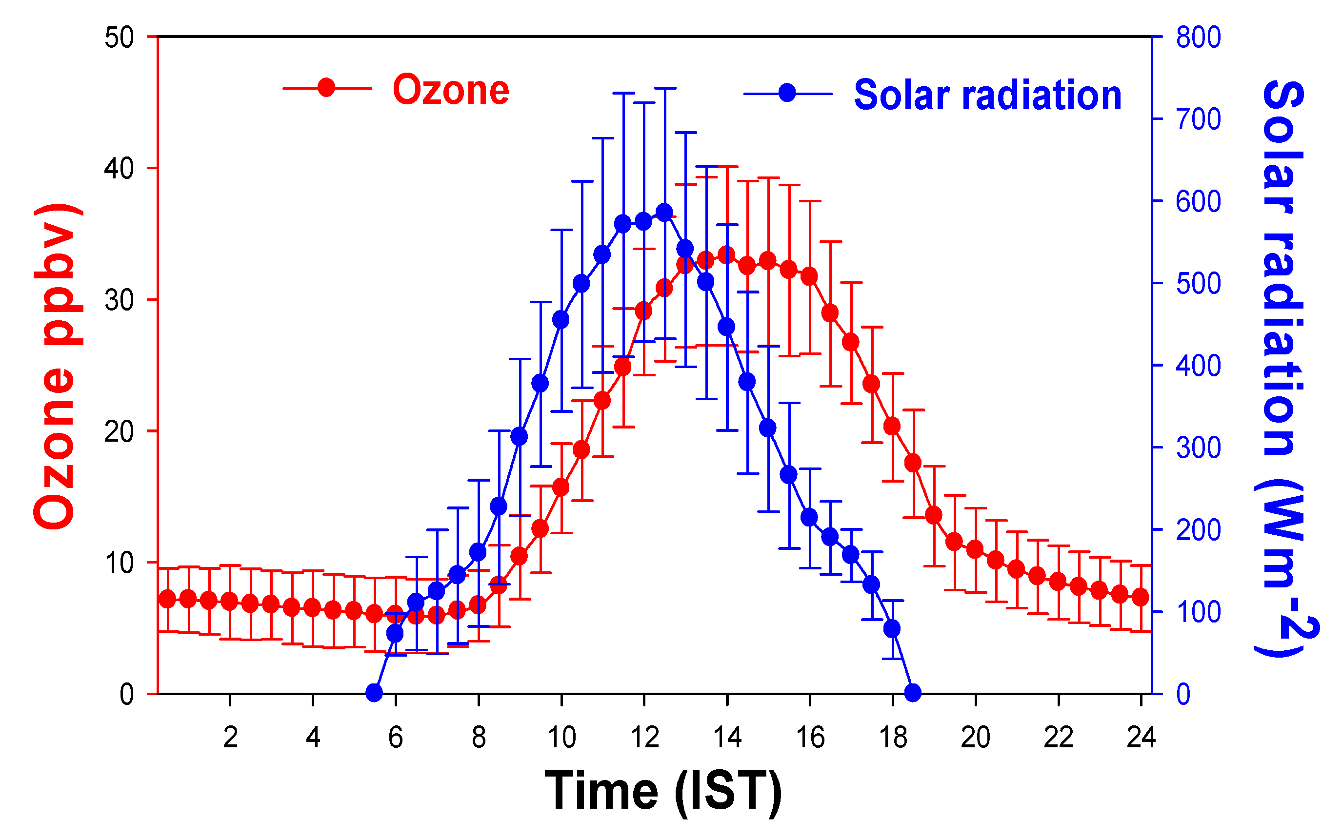
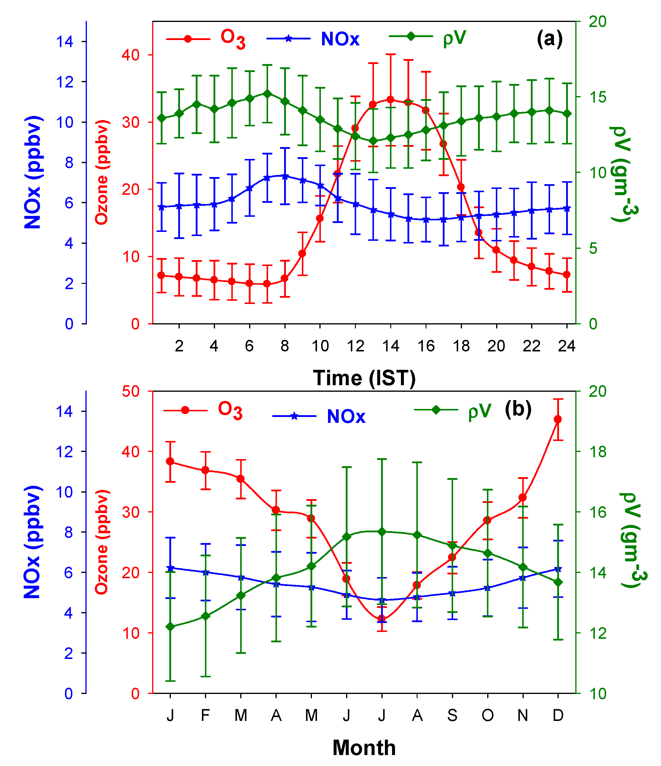
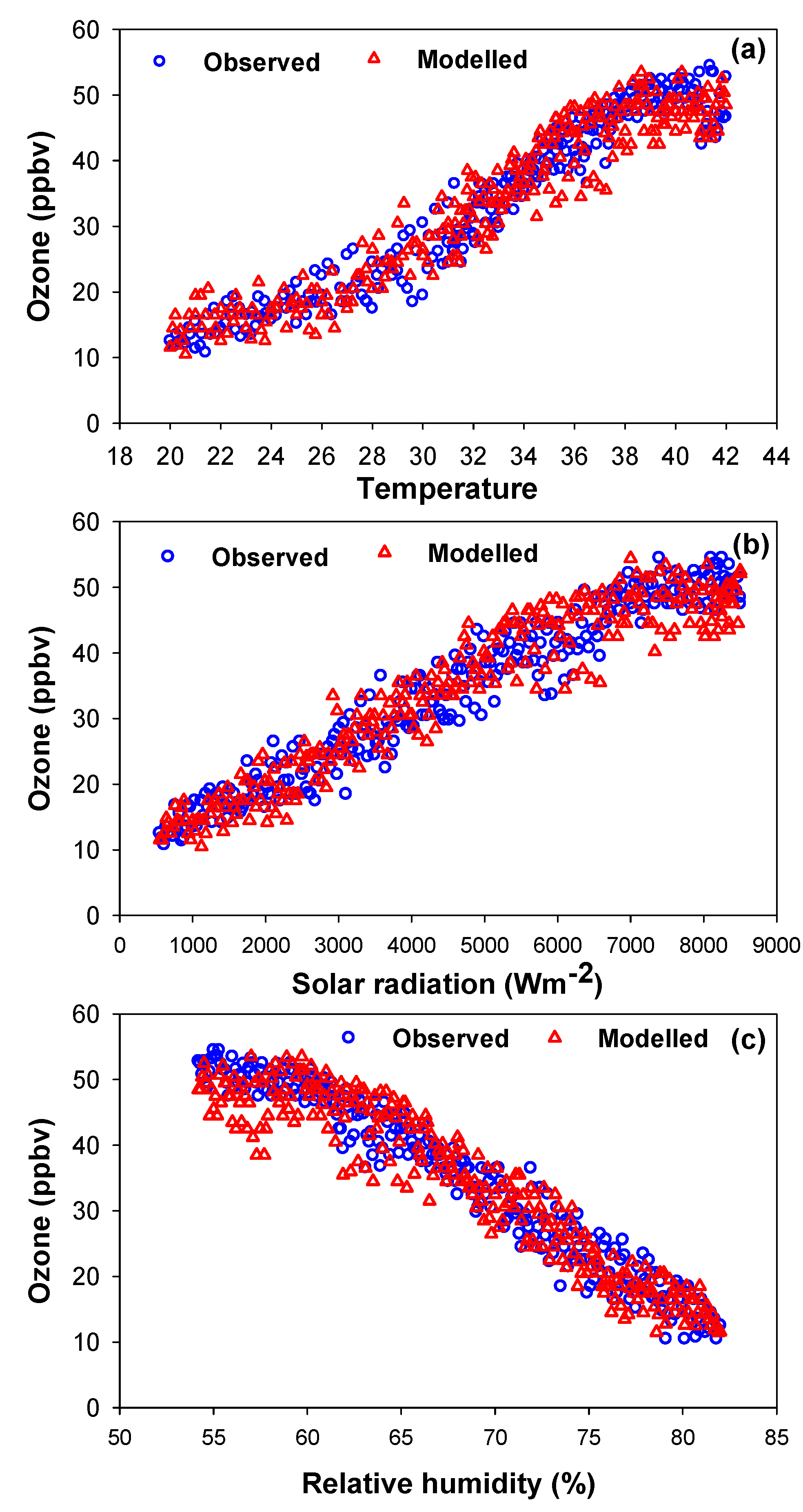
3.1. Influence of Solar Radiation and Water Vapor on O3 and NOx
3.2. Impact of Meteorological Parameters on O3 and NO2
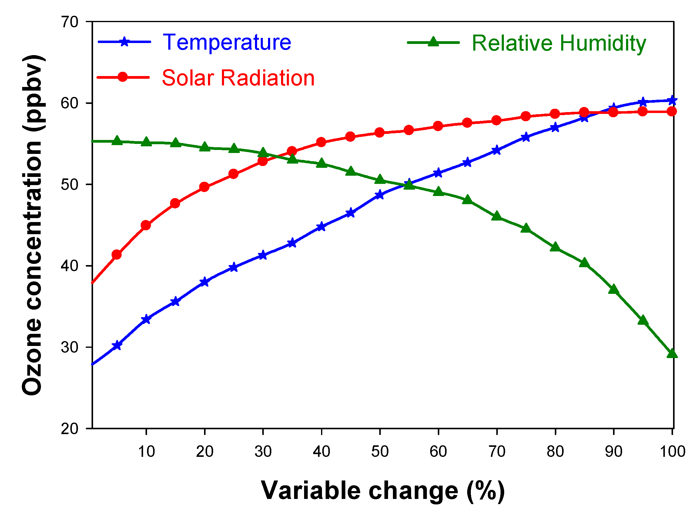
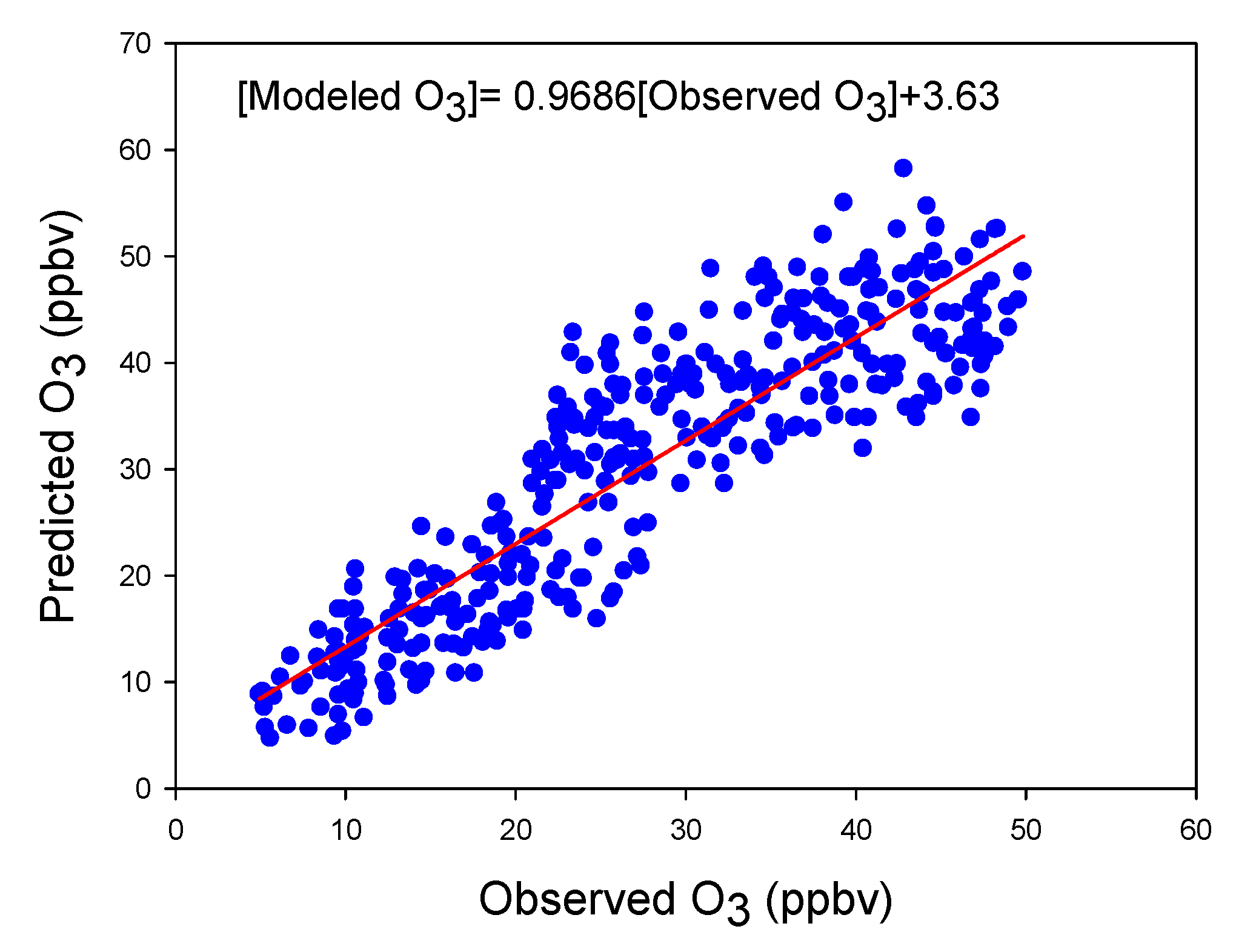
3.3. Impact of Air Temperature on O3 Production: A Neural Network Analysis
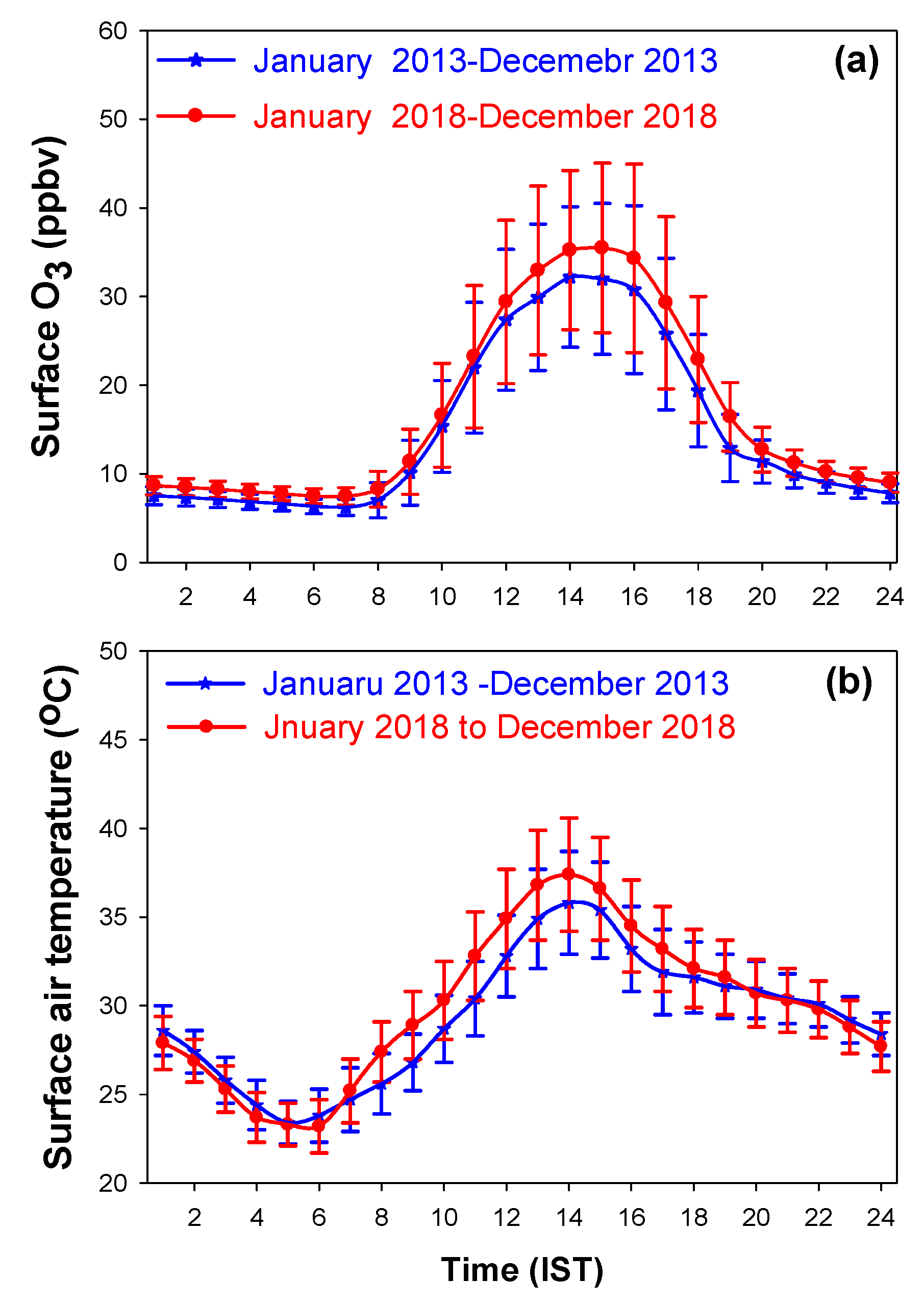
3.4. Long-Term Observed Variations of O3, NO, and NO2
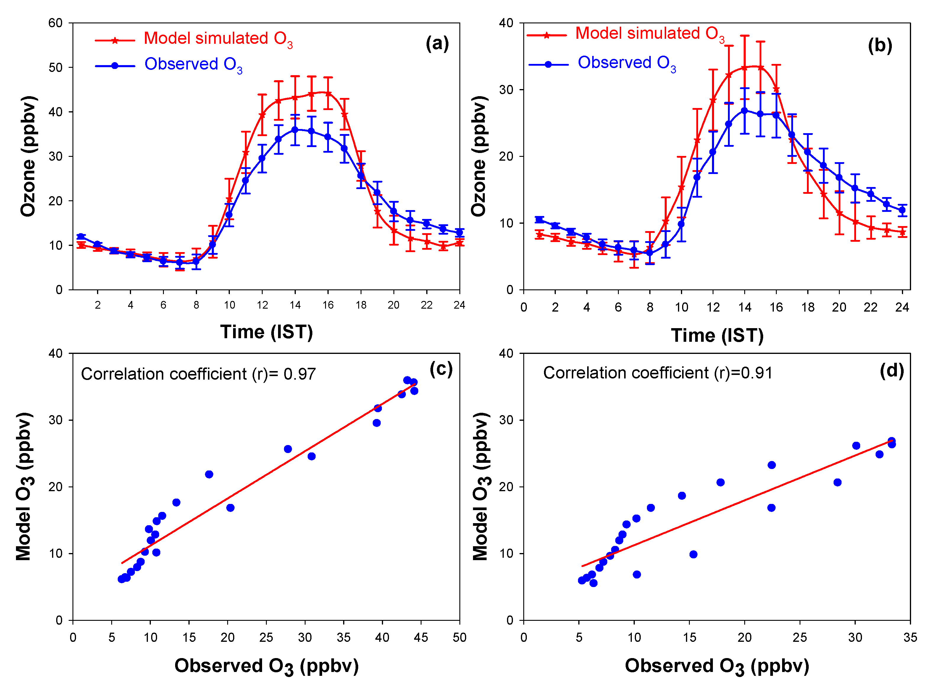
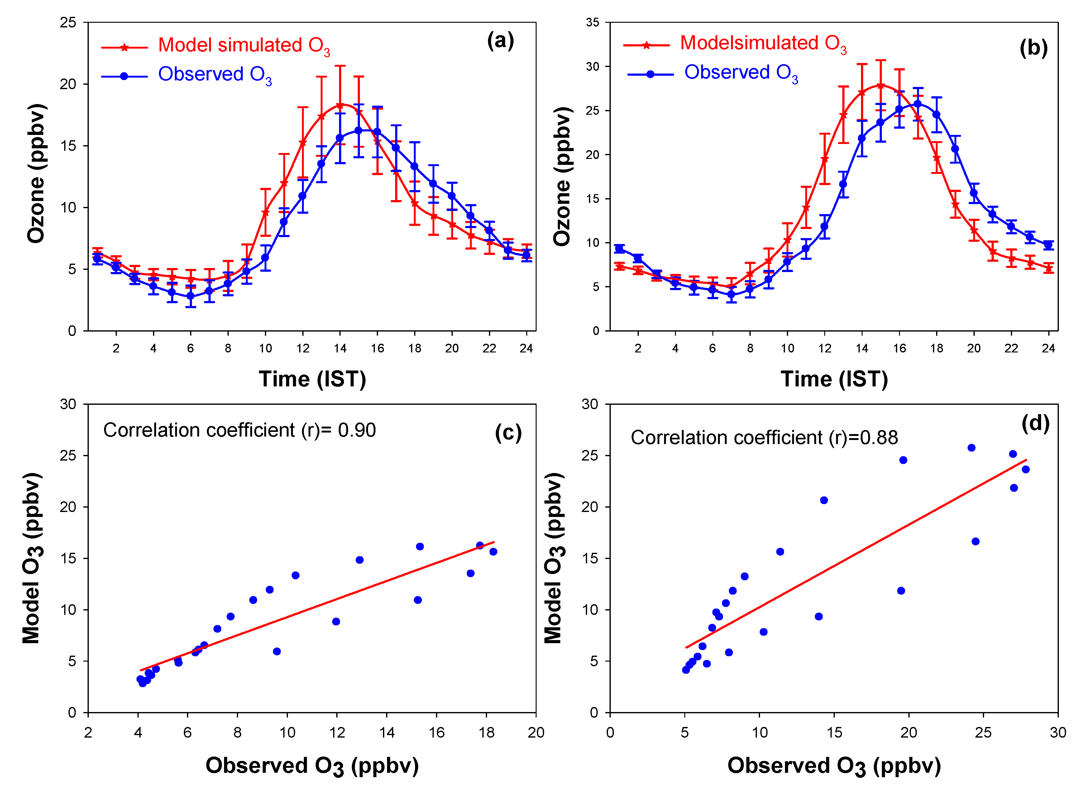
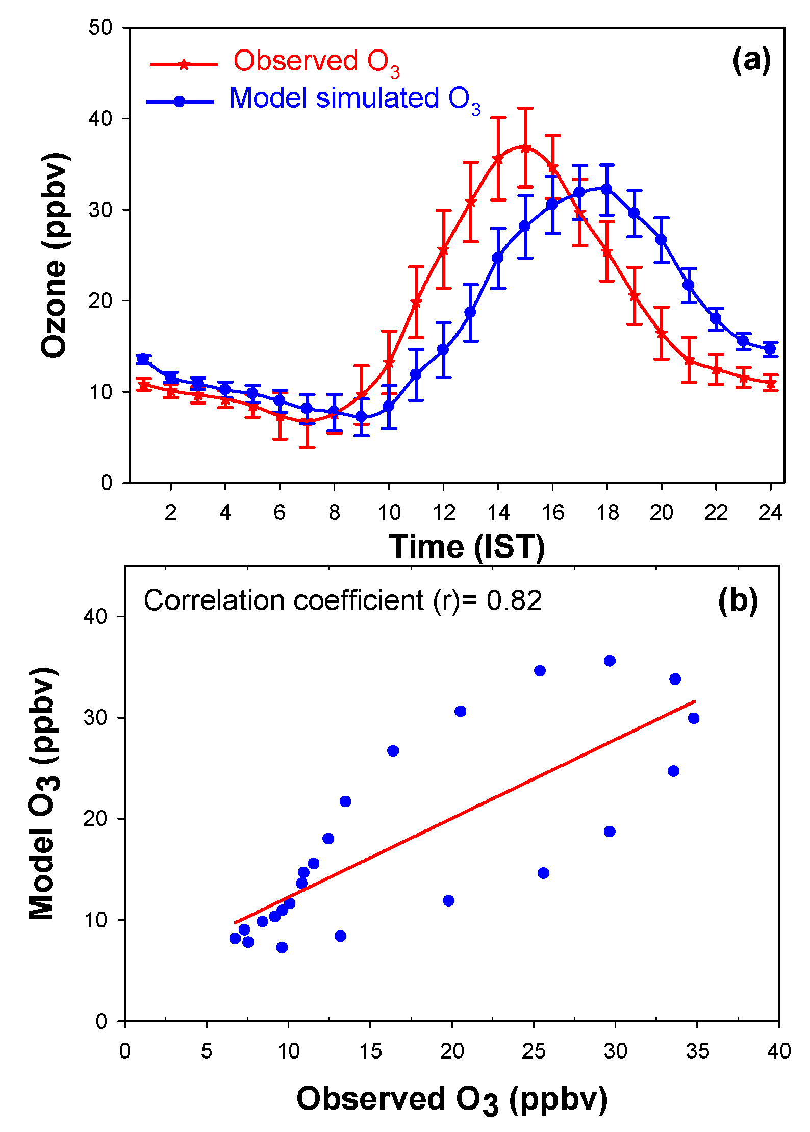
3.5. NCAR-MM Model Simulation
3.6. Comparison of O3 with Other Observational Sites
4. Conclusions
Author Contributions
Funding
Acknowledgments
Conflicts of Interest
References
- Cunningham, B.; Cunningham, M.A.; Saigo, B.W. Environmental Science: A Global Concern, 8th ed.; McGraw Hill: Boston, MA, USA, 2005. [Google Scholar]
- Ambient Air Pollution: A Global Assessment of Exposure and Burden of Disease: Geneva; World Health Organization (WHO) Library Cataloguing in Publication Data: Geneva, Switzerland, 2016.
- Kalpana, B.; Sagnik, D.; Tarun, G.; Dhaliwal, R.; Michael, B.; Aaron, J.; Jeffrey, D.; Gufran, B.; Tushar, K.J.; Ashutosh, N.A.; et al. The impact of air pollution on deaths, disease burden, and life expectancy across the states of India. Lancet Planet Health 2019, 3, 26–39. [Google Scholar]
- Debaje, S.B.; Kakade, A.D.; Jeyakumar, S.J. Air pollution effect of O3 on crop yield in rural India. J. Hazard. Mater. 2010, 183, 773–779. [Google Scholar] [CrossRef] [PubMed]
- Teixeira, E.; Fischer, G.; Velthuizen, H.V.; Dingenen, R.V.; Dentener, F.; Mills, G.; Walter, C.; Ewert, F. Limited potential of crop management for mitigating surface ozone impacts on global food supply. Atmos. Environ. 2011, 45, 2569–2576. [Google Scholar] [CrossRef]
- Wang, Y.; Hu, B.; Tang, G.; Ji, D.; Zhang, H.; Bai, J.; Wang, X.; Wang, Y. Characteristics of ozone and its precursors in Northern China: A comparative study of three sites. Atmos. Res. 2013, 132, 450–459. [Google Scholar] [CrossRef]
- Mabahwi, N.A.B.; Leh, O.L.H.; Omar, D. Human Health and Wellbeing: Human health effect of air pollution. Procedia-Soc. Behav. Sci. 2014, 153, 221–229. [Google Scholar] [CrossRef] [Green Version]
- Saini, R.; Taneja, A.; Singh, P. Surface ozone scenario and air quality in the north-central part of India. J. Environ. Sci. 2017, 59, 72–79. [Google Scholar] [CrossRef]
- Nevers, N.D. Air Pollution Control Engineering Seconded; McGraw-Hill Companies, Inc.: New York, NY, USA, 2000; pp. 571–573. [Google Scholar]
- Monks, P.S.; Archibald, A.T.; Colette, A.; Cooper, O.; Coyle, M.; Derwent, R.; Fowler, D.; Granier, C.; Law, K.S.; Mills, G.; et al. Tropospheric ozone and its precursors from the urban to the global scale from air quality to short-lived climate forcer. Atmos. Chem. Phys. 2015, 15, 8889–8973. [Google Scholar] [CrossRef] [Green Version]
- Sharma, A.; Sharma, S.K.; Mandal, T.K.R. Influence of ozone precursors and particulate matter on the variation of surface ozone at an urban site of Delhi India. Sustain. Environ. Res. 2016, 26, 76–83. [Google Scholar] [CrossRef] [Green Version]
- Volz, A.; Kley, D. Evaluation of the Montsouris series of ozone measurements made in the nineteenth century. Nature 1998, 332, 240–242. [Google Scholar] [CrossRef]
- Bonasoni, P.; Stohl, A.; Cristofanaelly, P.; Calzolari, F.; Colombo, T.; Evangelisti, F. Background ozone variations at Mt Cimone Station. Atmos. Environ. 2000, 34, 5183–5189. [Google Scholar] [CrossRef]
- Kumar, R.; Naja, M.; Venkataramani, S.; Wild, O. Variations in surface ozone at Naintail a high altitude site in the central Himalayas. J. Geophys. Res. 2010, 115, D16302. [Google Scholar] [CrossRef] [Green Version]
- David, L.M.; Nair, P.R. Tropospheric column O3 and NO2 over the Indian region observed by Ozone Monitoring Instrument (OMI): Seasonal changes and long term trends. Atmos. Environ. 2013, 65, 25–39. [Google Scholar] [CrossRef]
- Tiwari, S.; Srivastava, A.K.; Bisht, D.S.; Parmita, P.; Srivastava, M.K.; Attri, S.D. Diurnal and seasonal variations of black carbon and PM25 over New Delhi India: Influence of meteorology. Atmos. Res. 2013, 125, 50–62. [Google Scholar] [CrossRef]
- Ojha, N.; Naja, M.; Sarangi, T.; Kumar, R.; Bhardwaj, P.; Lal, S.; Venkataramani, S.; Sagar, R.; Kumar, A.; Chandola, H.C. On the processes influencing the vertical distribution of ozone over the central Himalayas: Analysis of yearlong ozonesonde observations. Atmos. Environ. 2014, 88, 201–211. [Google Scholar] [CrossRef]
- Thompson, M.L.; Reynolds, J.; Cox, L.H.; Guttorp, P.; Sampson, P.D. A review of statistical methods for the meteorological adjustment of tropospheric ozone. Atmos. Environ. 2001, 35, 617–630. [Google Scholar] [CrossRef]
- Srivastava, S.; Lal, S.; Naja, M.; Venkataramani, S.; Gupta, S. Influence of regional pollution and long range transport over Western India: Analysis of ozonesonde data. Atmos. Environ. 2012, 47, 174–182. [Google Scholar] [CrossRef]
- Mahapatra, P.S.; Panda, S.; Das, N.; Rath, S.; Das, T. Variation in black carbon mass concentration over an urban site in the eastern coastal plains of the Indian sub-continent. Theor. Appl. Clim. 2013, 117, 133–147. [Google Scholar] [CrossRef]
- Cassandra, V.H.; Munger, J.W.; Steven, C.W.; Zahniser, M.; Nelson, D.J.; McManus, B. Atmospheric reactive nitrogen concentration and flux budgets at a North eastern US forest site. Agric. For. Meteorol. 2006, 136, 159–174. [Google Scholar]
- Penga, Y.P.; Chena, K.S.; Laib, C.H.; Lua, P.J.; Kaoa, J.H. Concentrations of H2O2 and HNO3 and O3– VOCs–NOx sensitivity in ambient air in southern Taiwan. Atmos. Environ. 2006, 40, 6741–6751. [Google Scholar] [CrossRef]
- Raivonen, M.; Vesala, T.; Pirjola, L.; Altimir, N.; Keronen, P.; Kulmala, M.; Hari, P. Compensation point of NOx exchange: Net result of NOx consumption and production. Agric. For. Meteorol. 2009, 149, 1073–1081. [Google Scholar] [CrossRef]
- Swamy, Y.V.; Venkanna, R.; Nikhil1, G.N.; Chitanya, D.N.S.K.; Sinha, P.R.; Ramakrishna, M.; Rao, A.G. Impact of oxides of nitrogen volatile organic carbons and black carbon emissions on ozone weekend/weekday variations at a semiarid urban site in Hyderabad. Aerosol Air Qual. Res. 2012. [Google Scholar] [CrossRef] [Green Version]
- Tyagi, S.; Tiwari, S.; Mishra, A.; Hopke, P.K.; Attri, S.D.; Srivastava, A.K.; Bisht, D.S. Spatial variability of concentrations of gaseous pollutants across the national capital region of Delhi India. Atmos. Pollut. Res. 2016. [Google Scholar] [CrossRef] [Green Version]
- Kunhikrishnan, T.; Lawrence, M.G.; Kuhlmann, R.V.; Wenig, M.O.; Willem, A.; Asman, H.; Richter, A.; Burrows, J.P. Regional NOx emission strength for the Indian subcontinent and the impact of emissions from India and neigh boring countries on regional O3 chemistry. J. Geophys. Res. 2006, 109, D15301. [Google Scholar] [CrossRef]
- Van der A, R.J.; Eskes, H.J.; Boersma, K.F.; Van Noije, T.P.C.; Roozendael, V.M.; DeSmedt, I.; Peters, D.H.M.U.; Meijer, E.W. Trends seasonal variability and dominant NOx source derived from a ten-year record of NO2 measured from space. J. Geophys. Res. 2008, 113, D04302. [Google Scholar] [CrossRef]
- Rai, R.; Rajput, M.; Agrawal, M.; Agrawal, S.B. Gaseous air pollutants: A review on current and future trends of emissions and impact on agriculture. J. Sci. Res. 2011, 55, 77–102. [Google Scholar]
- Comrie, A.C.; Yarnal, B. Relationships between synoptic scale atmospheric circulation and ozone concentrations in metropolitan Pittsburgh Pennsylvania. Atmos. Environ. 1992, 26, 301–312. [Google Scholar] [CrossRef]
- Zhang, J.; Rao, S.T.; Daggupaty, S.M. Meteorological processes and ozone exceedances in the north-eastern United States during the 12–16 July 1995 episode. J. Appl. Meteorol. 1998, 37, 776–789. [Google Scholar] [CrossRef]
- Dueñas, C.; Fern’andez, M.C.; Caete, S.; Carretero, J.; Liger, E. Assessment of ozone variations and meteorological effects in an urban area in the Mediterranean Coast. Sci. Total Environ. 2002, 299, 97–113. [Google Scholar] [CrossRef]
- Camalier, L.; Cox, W.; Dolwick, P. The effects of meteorology on ozone in urban areas and their use in assessing ozone trends. Atmos. Environ. 2007, 41, 7127–7137. [Google Scholar] [CrossRef]
- Bloomfield, P.; Royle, J.A.; Steinberg, L.J.; Yang, Q. Accounting for meteorological effects in measuring urban ozone levels and trends. Atmos. Environ. 1996, 30, 3067–3077. [Google Scholar] [CrossRef]
- Olszyna, K.J.; Luria, M.; Meagher, J.F. The correlation of temperature and rural ozone levels in south-eastern USA. Atmos. Environ. 1997, 31, 3011–3022. [Google Scholar] [CrossRef]
- C’ardenas, L.M.; Austin, J.F.; Burgess, R.A. Correlations between CO, NOy, O3 and non-methane hydrocarbons and their relationships with meteorology during winter 1993 on the North Norfolk Coast UK. Atmos. Environ. 1998, 32, 3339–3351. [Google Scholar] [CrossRef]
- Tu, J.; Xia, Z.G.; Wang, H.; Li, W. Temporal variations in surface ozone and its precursors and meteorological effects at an urban site in China. Atmos. Res. 2007, 85, 310–337. [Google Scholar] [CrossRef]
- Patil, S.D.; Thompson, B.; Revadekar, J.V. On the variation of the tropospheric ozone over Indian region in relation to the meteorological parameters International. J. Remote Sens. 2009, 30, 2813–2826. [Google Scholar] [CrossRef]
- Khiem, M.; Ooka, R.; Huang, H.; Hayami, H.; Yoshikado, Y.; Kawamoto, Y. Analysis of the relationship between changes in meteorological conditions and the variation in summer Ozone Levels over the Central Kanto Area. Adv. Meteorol. 2010, 2010, 349248. [Google Scholar] [CrossRef] [Green Version]
- Aneja, V.P.; Businger, S.; Li, Z.; Ciaiborn, C.S.; Murthy, A. Ozone climatology at high elevations in the southern Appalachians. J. Geophys. Res. 1991, 96, 1007–1021. [Google Scholar] [CrossRef]
- Kourtidis, K.; Zerefos, C.; Rapsomanikis, S.; Simeonov, V.; Balis, D.; Perros, P.E. Regional levels of O3 in the troposphere over eastern Mediterranean. J. Geophys. Res. 2002, 107, 8140. [Google Scholar] [CrossRef]
- Zerefos, C.; Kourtidis, K.A.; Melas, D.; Balis, D.; Zanis, P.; Katsaros, L.; Mantis, H.T.; Repapis, C.; Isaksen, I.; Sundet, J.; et al. Photochemical activity and solar ultraviolet radiation modulation factors (PAUR): An overview of the project. J. Geophys. Res. 2002, 107, 8134. [Google Scholar] [CrossRef]
- Qin, Y.; Tonnesen, G.S.; Wang, Z. One-hour and eight-hour average O3 in the California south coast air quality management district: Trends in peak values and sensitivity to precursors. Atmos. Environ. 2004, 38, 2197–2207. [Google Scholar] [CrossRef]
- Mazzeo, A.N.; Venegas, E.L.; Choren, H. Analysis of NO NO2 O3 and NOx concentrations measured at a green area of Buenos Aires City during wintertime. Atmos. Environ. 2005, 39, 3055–3068. [Google Scholar] [CrossRef]
- Bossioli, E.; Tombrou, M.; Dandou, A.; Soulakellis, N. Simulation of the effects of critical factors on O3 formation and accumulation in the greater Athens area. J. Geophys. Res. 2007, 112, D02309. [Google Scholar] [CrossRef] [Green Version]
- Ordóñez, C.; Brunner, D.; Staehelin, J.; Hadjinicolaou, P.; Pyle, J.A.; Jonas, M.; Wernli, H.; Prevot, A.S.H. Strong influence of lowermost stratospheric ozone on lower tropospheric background ozone changes over Europe. Geophys. Res. Lett. 2007, 34, L07805. [Google Scholar] [CrossRef] [Green Version]
- Alvarez, R.; Weilenmann, M.; Favez, J.Y. Evidence of increased mass fraction of NO2 within real world NOx emissions of modern light vehicles derived from a reliable online measuring method. Atmos. Environ. 2008, 42, 4699–4707. [Google Scholar] [CrossRef]
- Shan, W.; Yin, Y.; Zhang, J.; Ji, X.; Deng, X. Surface ozone and meteorological condition in a single year at an urban site in central–eastern China. Environ. Monit. Assess. 2009, 151, 127–141. [Google Scholar] [CrossRef]
- Solberg, S.; HovØSovde, A.; Isaksen, I.S.A.; Coddeville, P.; De Backer, H.; Forster, C.; Orsolini, Y.; Uhse, K. European surface ozone in the extreme summer 2003. J. Geophys. Res. 2008, 113, D07307. [Google Scholar] [CrossRef] [Green Version]
- Yarwood, N.G.; Grant, J.; Koo, B.; Dunker, A.M. Modeling weekday to weekend changes in emissions and O3 in the Los Angeles basin for 1997 and 2010. Atmos. Environ. 2008, 42, 3765–3779. [Google Scholar] [CrossRef]
- Yin, Y.; Shan, W.; Ji, X.; Deng, X.; Cheng, J.; Li, L. Analysis of the surface ozone during summer and autumn at a coastal site in East China. Bull. Environ. Contam. Toxicol. 2010, 85, 10–14. [Google Scholar] [CrossRef]
- Song, F.; Shin, J.Y.; Atresino, R.J.; Gao, Y. Relationships among the spring time ground-level NOx O3 and NO3 in the vicinity of highways in the US East Coast. Atmos. Pollut. Res. 2011, 2, 374–383. [Google Scholar] [CrossRef] [Green Version]
- Wallace, H.W.; Jobson, B.T.; Erickson, M.H.; McCoskey, J.K.; VanReken, T.M.; Lamb, B.K.; Vaughan, J.K.; Hardy, R.J.; Cole, J.L.; Strachan, S.M.; et al. Comparison of wintertime CO to NOx ratios to MOVES and MOBILE62 on-road emissions inventories. Atmos. Environ. 2012, 63, 289–297. [Google Scholar] [CrossRef]
- Henschel, S.; Querol, X.; Atkinson, R.; Pandolfi, M.; Zeka, A.; Tertre, A.; Analitis, A.; Katsouyanni, K.; Chanel, O.; Pascal, M.; et al. Ambient air SO2 patterns in 6 European cities. Atmos. Environ. 2013, 79, 236–247. [Google Scholar] [CrossRef]
- Han, S.; Zhang, M.; Zhao, C.; Lu, X.; Ran, L.; Han, M.; Li, P.; Li, X. Differences in ozone photochemical characteristics between the megacity Tianjin and its rural surroundings. Atmos. Environ. 2013, 79, 209–216. [Google Scholar] [CrossRef]
- Sun, Y.; Zhou, X.; Wai, K.; Yuan, Q.; Xu, Z.; Zhou, S.; Qi, Q.; Wang, W. Simultaneous measurement of particulate and gaseous pollutants in an urban city in North China Plain during the heating period: Implication of source contribution. Atmos. Res. 2013, 134, 24–34. [Google Scholar] [CrossRef]
- Lurmann, F.W.; Wexler, A.S.; Pandis, S.N.; Mussara, S.; Kumar, N.; Seinfeld, J.H. Modelling Urban and Regional Aerosols—II Application to California’s South Coast Air Basin. Atmos. Environ. 1997, 31, 2695–2715. [Google Scholar] [CrossRef]
- Pai, P.; Vijayaraghavan, K.; Seigneur, C. Particulate matter modeling in the Los Angeles basin using the SAQM-AERO. J. Air Waste Manag. Assoc. 2000, 50, 32–42. [Google Scholar] [CrossRef] [Green Version]
- Lazaridis, M.; Spyridaki, A.; Solberg, S.; Smolik, J.; Zdimal, V.; Eleftheriadis, K. Mesoscale modeling of combined aerosol and photo-oxidant processes in the Eastern Mediterranean. Atmos. Chem. Phys. 2005, 5, 927–940. [Google Scholar] [CrossRef] [Green Version]
- Resmi, C.T.; Nishanth, T.; Kumar, M.K.S.; Balachandramohan, M.; Valsaraj, K.T. Temporal changes in air quality during a festival season in Kannur India. Atmosphere 2019, 10, 137. [Google Scholar] [CrossRef]
- Lingaswamy, A.P.; Arafath, S.M.; Balakrishnaiah, G.; Rama Gopal, K.; Reddy, N.S.K.; Reddy, K.R.O.; Reddy, R.R.; Rao, T.C. Observations of trace gases photolysis rate coefficients and model simulations over semi-arid region India. Atmos. Environ. 2017, 158, 246–258. [Google Scholar] [CrossRef]
- Rama Gopal, K.; Lingaswamy, A.P.; Arafath, S.M.D.; Balakrishnaiah, G.; Pavan, K.S.; Devi, U.K.; Reddy, N.S.K.; Reddy, K.R.O.; Reddy, R.R.; Lal, S. Seasonal heterogeneity in ozone and its precursors (NOx) by in-situ and model observations on semi-arid station in Anantapur (AP). Atmos. Environ. 2014, 84, 294–306. [Google Scholar] [CrossRef]
- Ojha, N.; Naja, M.; Singh, K.P.; Sarangi, T.; Kumar, R.; Lal, S.; Lawrence, M.G.; Butler, T.M. Variabilities in O3 at a semi-urban site in the Indo-Gangetic Plain region: Association with the meteorology and regional processes. J. Geophys. Res. 2012, 117, D20301. [Google Scholar] [CrossRef]
- Nair, P.R.; David, L.M.; Girach, I.A.; George, S.K. Ozone in the marine boundary layer of Bay of Bengal during post-winter period: Spatial pattern and role of meteorology. Atmos. Environ. 2011, 45, 4671–4681. [Google Scholar] [CrossRef]
- Girach, I.A.; Nair, P.R.; David, L.M.; Hegde, P.; Mishra, M.K.; Kumar, M.G.; Das, M.S.; Ojha, N.; Naja, M. The changes in near-surface ozone and precursors at two nearby tropical sites during annular solar eclipse of 15 January 2010. J. Geophys. Res. 2012, 117, D01303. [Google Scholar] [CrossRef]
- Nishanth, T.; Praseed, K.M.; Kumar, M.K.S.; Valsaraj, K.T. Influence of ozone precursors and PM10 on the variation of surface O3 over Kannur India. Atmos. Res. 2014, 138, 112–124. [Google Scholar] [CrossRef]
- Shan, W.; Yin, Y.; Zhang, J.; Ding, Y. Observational study of surface O3 at an urban site in East China. Atmos. Res. 2008, 89, 252–261. [Google Scholar] [CrossRef]
- Chakraborty, K.; Mehrotra, K.; Mohan, C.K.; Ranka, S. Forecasting the behavior of multivariate time series using neural networks. Neural Netw. 1992, 5, 961–970. [Google Scholar] [CrossRef] [Green Version]
- Narasimhan, R.; Keller, J.; Subramaniam, G. Ozone modelling using neural networks. J. Appl. Meteorol. 2000, 39, 291–296. [Google Scholar] [CrossRef]
- Faris, H.; Alkasassbeh, M.; Rodan, A. Artificial Neural Networks for Surface Ozone Prediction: Models and Analysis. Pol. J. Environ. Stud. 2014, 23, 341–348. [Google Scholar]
- Kleinman, L.; Lee, Y.N.; Springston, S.R.; Nunnermacker, L.; Zhou, X.; Brown, R.; Hallock, K.; Klotz, P.; Leahy, D.; Lee, J.H.; et al. Ozone formation at a rural site in the southern United States. J. Geophys. Res. 1994, 99, 3469–3482. [Google Scholar] [CrossRef]
- Kneizys, F.X.; Shettle, E.P.; Gallery, W.O.; Chetwynd, J.H., Jr.; Abreu, L.W.; Selby, J.E.A.; Fenn, R.W.; McClatchey, R.A. Atmospheric Transmittance/radiance: Computer code LOWTRAN 5; AFGLTR-80-0067 AD088215; Optical Physics Division, Air Force Geophysics Laboratory: Wright-Patterson Air Force Base, OH, USA, 1980. [Google Scholar]
- Pancholi, P.; Kumar, A.; Bikundia, D.S.; Chourasiya, S. An observation of seasonal and diurnal behavior of O3-NOx relationships and local/regional oxidant (OX = O3 + NO2) levels at a semi-arid urban site of western India. Sustain. Environ. Res. 2018, 28, 79–89. [Google Scholar] [CrossRef]
- Yadav, R.; Sahu, L.K.; Beig, G.; Jaaffrey, S.N.A. Role of long-range transport and local meteorology in seasonal variation of surface ozone and its precursors at an urban site of India. Atmos. Res. 2016. [Google Scholar] [CrossRef]
- Li, J.; Wang, Z.; Wang, X.; Yamaji, K.; Takigawa, M.; Kanaya, Y.; Pochanart, P.; Liu, Y.; Irie, H.; Hu, B.; et al. Impacts of aerosols on summertime tropospheric photolysis frequencies and photochemistry over Central Eastern China. Atmos. Environ. 2011, 45, 1817–1829. [Google Scholar] [CrossRef]
- Bian, H.; Han, S.Q.; Tie, X.X.; Sun, M.L.; Liu, A.X. Evidence of impact of aerosols on surface ozone concentration in Tianjin China. Atmos. Environ. 2007, 41, 4672–4681. [Google Scholar] [CrossRef]
- Reddy, B.S.K.; Kumar, K.R.; Balakrishnaiah, G.; Gopal, K.R.; Reddy, R.R.; Sivakumar, V.; Lingaswamy, A.P.; Arafath, S.M.; Umadevi, K.; Pavan, K.S.; et al. Analysis of diurnal and seasonal behavior of surface ozone and its precursors (NOx) at a semi-arid rural site in Southern India. Aerosol Air Qual. Res. 2012, 12, 1081–1094. [Google Scholar] [CrossRef] [Green Version]
- Evans, S.J.; Toumi, R.; Harries, J.E.; Chipperfield, M.P.; Russel, J.M. Trends in stratospheric humidity and the sensitivity of ozone to these trends. J. Geophys. Res. 1998, 103, 8715–8725. [Google Scholar] [CrossRef] [Green Version]
- Kirk Davidoff, D.B.; Hintsa, E.J.; Anderson, G.; Keith, D.W. The effect of climate change of ozone depeletion through changes in stratospheric water vapour. Nature 1999, 402, 399–401. [Google Scholar] [CrossRef]
- Foster, P.M.; De, F.; Shine, K.P. Assessing the climate impact of trend in stratospheric water vapour. Geophys. Res. Lett. 2002, 29. [Google Scholar] [CrossRef] [Green Version]
- Lu, X.; Zhang, L.; Shen, L. Meteorology and Climate Influences on Tropospheric Ozone: A Review of Natural Sources Chemistry and Transport Patterns. Curr. Pollut. Rep. 2019, 1–23. [Google Scholar] [CrossRef] [Green Version]
- Pyrgou, A.; Hadjinicolaou, P.; Santamouris, M. Enhanced near-surface ozone under heat wave conditions in a Mediterranean island. Nature 2018, 8, 9191. [Google Scholar] [CrossRef] [Green Version]
- Buhr, M.P.; Hsu, K.J.; Liu, C.M.; Liu, R.; Wei, L.; Liu, Y.C.; Kuo, S. Trace gas measurements and air mass classification from a ground station in Taiwan during the PEM-WEST experiment. J. Geophys. Res. 1995, 101, 2025–2035. [Google Scholar] [CrossRef]
- Sillman, S.; Samson, P.J. Impact of temperature on oxidant photochemistry in urban polluted rural and remote environments. J. Geophys. Res. 1995, 100, 11497–11508. [Google Scholar] [CrossRef]
- Steiner, A.L.; Tonse, S.; Cohen, R.C.; Goldstein, A.H.; Harley, R. Influence of future climate and emissions on regional air quality in California. J. Geophys. Res. 2006, 111, D18303. [Google Scholar] [CrossRef]
- Stathopoulou, E.; Mihalakakou, G.; Santamouris, M.; Bagiorgas, H.S. On the impact of temperature on tropospheric Ozone concentration levels in urban environments. J. Earth Syst. Sci. 2008, 117, 227–236. [Google Scholar] [CrossRef]
- De Miguel, A.; Mateos, D.; Bilbao, J.; Román, R. Sensitivity analysis of ratio between ultraviolet and total shortwave solar radiation to cloudiness ozone aerosols and precipitable water. Atmos. Res. 2011, 102, 136–144. [Google Scholar] [CrossRef]
- Kleanthous, S.; Vrekoussis, M.; Mihalopoulos, N.; Kalabokas, P.; Lelieveld, J. On the temporal and spatial variation of ozone in Cyprus. Sci. Total Environ. 2014, 476, 677–687. [Google Scholar] [CrossRef] [PubMed]
- Lee, Y.C.; Shindell, D.T.; Faluvegi, G.; Wenig, M.; Lam, Y.F.; Ning, Z.; Hao, S.; Lai, C.S. Increase of ozone concentrations its temperature sensitivity and the precursor factor in South China. Tellus B 2014, 66, 23455. [Google Scholar] [CrossRef]
- Pusede, S.E.; Steiner, A.L.; Cohen, R.C. Temperature and recent trends in the chemistry of continental surface ozone. Chem. Rev. 2015, 115, 3898–3918. [Google Scholar] [CrossRef]
- Coates, J.; Mar, K.A.; Ojha, N.; Butler, T.M. The influence of temperature on ozone production under varying NOx conditions-A modelling study. Atmos. Chem. Phys. 2016, 16, 11601–11615. [Google Scholar] [CrossRef] [Green Version]
- Porter, W.C.; Heald, C.L. The mechanisms and meteorological drivers of the ozone temperature relationship. Atmos. Chem. Phys. Discuss. 2019. [Google Scholar] [CrossRef] [Green Version]
- Dawson, J.P.; Adams, P.J.; Pandis, S.N. Sensitivity of ozone to summertime climate in the eastern USA: A modeling case study. Atmos. Environ. 2007, 41, 1494–1511. [Google Scholar] [CrossRef]
- Wu, S.; Mickley, L.J.; Leibensperger, E.M.; Jacob, D.J.; Rind, D.; Streets, D.G. Effects of 2000–2050 global change on ozone air quality in the United States. J. Geophys. Res. 2008, 113. [Google Scholar] [CrossRef] [Green Version]
- Mckendry, I.G. Synoptic circulation and summer time ground level ozone concentrations at Vancouver British Colombia. J. Appl. Metrol. 1994, 33, 627–641. [Google Scholar] [CrossRef] [Green Version]
- Kumar, R.; Barth, M.C.; Pfister, G.G.; Monache, L.D.; Lamarque, J.F.; Nicholls, A.S.; Tilmes, S.; Ghude, S.D.; Wiedinmyer, C.; Naja, M.; et al. How Will Air Quality Change in South Asia by 2050? J. Geophys. Res. 2018, 123, 1840–1864. [Google Scholar] [CrossRef]
- Yamaji, K.; Ohara, T.; Uno, I.; Kurokawa, J.; Pochanart, P.; Akimoto, H. Future prediction of surface ozone over east Asia using models-3 community multiscale air quality modeling system and regional emission inventory in Asia. J. Geophys. Res. 2008, 113, D08306. [Google Scholar] [CrossRef]
- Barnard, J.C.; Chapman, E.G.; Fast, J.D.; Schmelzer, J.R.; Slusser, J.R.; Shetter, R.E. An evaluation of the FAST-J photolysis algorithm for predicting nitrogen dioxide photolysis rates under clear and cloudy conditions. Atmos. Environ. 2004, 38, 3393–3403. [Google Scholar] [CrossRef]
- Gustavo, G.P.; Rafael, P.F.; Beatriz, M.T. Photolysis rate coefficients calculations from broadband UV-B irradiance: Model-measurement interaction. Atmos. Environ. 2005, 39, 857–866. [Google Scholar]
- Aumont, B.; Madronich, S.; Bey, I.; Tyndall, G.S. Contribution of secondary VOC to the composition of aqueous atmospheric particles: A modelling approach. J. Atmos. Chem. 2000, 35, 59–75. [Google Scholar] [CrossRef]
- Madronich, S. Chemical evolution of gaseous air pollutants down-wind of tropical megacities: Mexico City case study. Atmos. Environ. 2006, 40, 6012–6018. [Google Scholar] [CrossRef]
- Ahammed, Y.N.; Reddy, R.R.; Gopal, K.R. Seasonal variation of the surface ozone and its precursor gases during 2001- 2003, measured at Anantapur (14.62N), a semi-arid site in India. Atmos. Res. 2006, 80, 151–164. [Google Scholar] [CrossRef]
- Beig, G.; Gunthe, S.; Jadhav, D.B. Simultaneous measurements of ozone and its precursors on a diurnal scale at a semi urban site in India. J. Atmos. Chem. 2007, 57, 239–253. [Google Scholar] [CrossRef]
- Bhuyan, P.K.; Bharali, C.; Pathak, B.; Kalita, G. The role of precursor gases and meteorology on temporal evolution of O3 at a tropical location in northeast India. Environ. Sci. Pollut. Res. 2014, 21, 6696–6713. [Google Scholar] [CrossRef]
- Datta, A.; Saud, T.; Goel, A.; Tiwari, S.; Sharma, S.K.; Saxena, M.; Mandal, T.K. Variation of ambient SO2 over Delhi. J. Atmos. Chem. 2011, 65, 127–143. [Google Scholar] [CrossRef]
- Debaje, S.B.; Kakade, A.D. Surface O3 variability over western Maharashtra, India. J. Hazard. Mater. 2009, 161, 686–700. [Google Scholar] [CrossRef] [PubMed]
- Debaje, S.; Jeyakumar, S.J. High O3 at coastal sites in India. Int. J. Remote Sens. 2011, 32, 993–1015. [Google Scholar] [CrossRef]
- Ghude, D.; Jain, S.L.; Arya, B.C.; Beig, G.; Ahammed, Y.N.; Kumar, A.; Tyagi, B. O3 in ambient air at a tropical megacity, Delhi: Characteristics, trends and cumulative O3 exposure indices. J. Atmos. Chem. 2008, 60, 237–252. [Google Scholar] [CrossRef]
- Jain, S.L.; Arya, B.C.; Kumar, A.; Ghude, S.D.; Kulkarni, P.S. Observational study of surface O3 at New Delhi, India. Int. J. Remote Sens. 2005, 26, 3515–3524. [Google Scholar] [CrossRef]
- Lal, S.; Naja, M.; Subbaraya, B.H. Seasonal variations in surface ozone and its precursors over an urban site in India. Atmos. Environ. 2000, 34, 2713–2724. [Google Scholar] [CrossRef]
- Lal, S.; Sahu, L.K.; Gupta, S.; Srivastava, S.; Modh, K.S.; Venkataramani, S.; Rajesh, T.A. Emission characteristic of O3 related trace gases at a semi-urban site in the Indo-Gangetic plain using intercorrelations. J. Atmos. Chem. 2008, 60, 189–204. [Google Scholar] [CrossRef]
- Nair, P.R.; Ajayakumar, R.S.; David, L.M.; Girach, I.A.; Mottungan, K. Decadal changes in surface ozone at the tropical station Thiruvananthapuram (8.542° N, 76.858° E), India: Effects of anthropogenic activities and meteorological variability. Environ. Sci. Pollut. Res. 2018, 25, 14827–14843. [Google Scholar] [CrossRef]
- Naja, M.; Lal, S.; Chand, D. Diurnal and seasonal variabilities in surface O3 at ahigh altitude site Mt Abu (24.60 N, 72.70 E, 1680 m asl) in India. Atmos. Environ. 2003, 37, 4205–4215. [Google Scholar] [CrossRef]
- Nishanth, T.; Praseed, K.M.; Satheesh Kumar, M.K.; Valsaraj, K.T. Observational study of surface O3, NOx, CH4 and total NMHC’s at Kannur, India. Aerosol Air Qual. Res. 2014, 14, 1074–1088. [Google Scholar] [CrossRef]
- Pulikesi, M.; Baskaralingam, P.; Rayudu, V.N.; Elango, D.; Ramamurthi, V.; Sivanesan, S. Surface O3 measurements at urban coastal site Chennai, in India. J. Hazard. Mater. 2006, 137, 1554–1559. [Google Scholar] [CrossRef]
- Purkait, N.N.; De, S.; Sen, S.; Chakrabarty, D.K. Surface O3 and its precursors at two sites in the north east coast of India. Indian. J. Radio Space Phys. 2009, 38, 86–97. [Google Scholar]
- Sharma, P.; Kuniyal, J.C.; Chand, K.; Guleria, R.P.; Dhyani, P.P.; Chauhan, C. Surface O3 concentration and its behaviour with aerosols in the north western Himalaya, India. Atmos. Environ. 2013, 71, 44–53. [Google Scholar] [CrossRef]
- Singla, V.; Satsangi, A.; Pachauri, T.; Lakhani, A.; Kumari, K.M. O3 formation and destruction at a sub-urban site in North Central region of India. Atmos. Res. 2011, 101, 373–385. [Google Scholar] [CrossRef]
- Tiwari, S.; Rai, R.; Agrawal, M. Annual and seasonal variations in tropospheric O3 concentrations around Varanasi. Int. J. Remote Sens. 2008, 29, 4499–4514. [Google Scholar] [CrossRef]
- Mandal, T.K.; Peshin, S.K.; Sharma, C.; Gupta, P.K.; Raj, R.; Sharma, S.K. Study of surface ozone at Port Blair, India, a remote marine station in the Bay of Bengal. J. Atmos. Solar-Terr. Phys. 2015, 129, 142–152. [Google Scholar] [CrossRef]
- Gaur, A.; Tripathi, S.N.; Kanawade, V.P.; Tare, V.; Shukla, S.P. Four-year measurements of trace gases (SO2, NOx, CO, and O3) at an urban location, Kanpur, in Northern India. J. Atmos. Chem. 2014, 71, 283–301. [Google Scholar] [CrossRef]
- Mahapatra, P.S.; Panda, S.; Walvekar, P.P.; Kumar, R.; Das, T.; Gurjar, B.R. Seasonal trends, meteorological impacts, and associated health risks with atmospheric concentrations of gaseous pollutants at an Indian coastal city. Environ. Sci. Pollut. Res. 2014. [Google Scholar] [CrossRef]
- Udayasoorian, C.; Jayabalakrishnan, R.M.; Suguna, A.R.; Venkataramani, S.; Lal, S. Diurnal and seasonal characteristics of ozone and NOx over a high altitude Western Ghats location in Southern India. Adv. Appl. Sci. Res. 2013, 4, 309–320. [Google Scholar]


| Parameters | O3 | NO2 | Temperature | Solar Radiation | RH | Wind Velocity |
|---|---|---|---|---|---|---|
| O3 | 1 | 0.68 | 0.89 | 0.74 | −0.82 | −0.76 |
| NO2 | 0.68 | 1 | −0.62 | −0.48 | −0.44 | −0.38 |
| Temperature | 0.89 | −0.62 | 1 | 0.64 | −0.48 | −0.42 |
| Solar radiation | 0.74 | −0.48 | 0.64 | 1 | −0.54 | −0.38 |
| Relative humidity | −0.82 | −0.44 | -0.48 | −0.54 | 1 | −0.36 |
| Wind speed | −0.76 | −0.38 | −0.42 | −0.38 | −0.36 | 1 |
| Parameters | Minimum | Maximum | Average |
|---|---|---|---|
| Ozone (ppbv) | 10 | 50 | 30 |
| Total ozone column (DU) | 200 | 280 | 240 |
| NO (ppbv) | 0.5 | 3 | 2 |
| NO2 (ppbv) | 0.5 | 5 | 3 |
| Surface air temperature (°C) | 16 | 44 | 25 |
| Relative humidity (%) | 40 | 90 | 65 |
| Solar radiation (Wm−2) | 0 | 900 | 400 |
| Wind speed (ms−1) | 0 | 10 | 2 |
| Time | O3 (ppbv) | NO (ppbv) | NO2 (ppbv) |
|---|---|---|---|
| 1 | 5.79 ± 1.05 | 1.67 ± 0.22 | 1.89 ± 0.28 |
| 2 | 5.66 ± 0.90 | 1.65 ± 0.30 | 1.91 ± 0.36 |
| 3 | 5.49 ± 0.88 | 1.64 ± 0.35 | 1.90 ± 0.42 |
| 4 | 5.29 ± 0.88 | 1.65 ± 0.37 | 1.90 ± 0.44 |
| 5 | 5.06 ± 0.82 | 1.61 ± 0.41 | 1.90 ± 0.47 |
| 6 | 4.77 ± 0.90 | 1.56 ± 0.38 | 1.88 ± 0.48 |
| 7 | 4.57 ± 0.80 | 1.56 ± 0.32 | 1.93 ± 0.50 |
| 8 | 5.50 ± 1.63 | 1.67 ± 0.38 | 2.06 ± 0.50 |
| 9 | 8.76 ± 3.15 | 1.81 ± 0.42 | 2.22 ± 0.46 |
| 10 | 13.99 ± 5.74 | 1.85 ± 0.50 | 2.22 ± 0.39 |
| 11 | 20.33 ± 8.74 | 1.71 ± 0.51 | 1.99 ± 0.42 |
| 12 | 26.06 ± 10.43 | 1.55 ± 0.48 | 1.75 ± 0.43 |
| 13 | 30.04 ± 10.72 | 1.36 ± 0.41 | 1.53 ± 0.39 |
| 14 | 31.42 ± 10.48 | 1.13 ± 0.25 | 1.35 ± 0.39 |
| 15 | 32.29 ± 11.09 | 1.05 ± 0.23 | 1.25 ± 0.43 |
| 16 | 30.51 ± 11.80 | 1.04 ± 0.22 | 1.21 ± 0.44 |
| 17 | 25.63 ± 11.11 | 1.12 ± 0.25 | 1.24 ± 0.40 |
| 18 | 19.23 ± 7.55 | 1.24 ± 0.30 | 1.3 ± 0.34 |
| 19 | 12.79 ± 3.88 | 1.35 ± 0.31 | 1.44 ± 0.28 |
| 20 | 9.95 ± 2.35 | 1.46 ± 0.30 | 1.57 ± 0.27 |
| 21 | 8.45 ± 1.36 | 1.55 ± 0.31 | 1.66 ± 0.28 |
| 22 | 7.50 ± 1.07 | 1.64 ± 0.33 | 1.76 ± 0.30 |
| 23 | 6.83 ± 1.04 | 1.75 ± 0.33 | 1.89 ± 0.30 |
| 24 | 6.30 ± 1.10 | 1.84 ± 0.34 | 2.17 ± 0.29 |
| Duration | Statistics | Gases | |||
|---|---|---|---|---|---|
| O3 | NO | NO2 | NOx | ||
| 1 January 2013– 31 December 2013 | Average | 31.97 | 2.19 | 2.32 | 4.51 |
| Standard deviation | 8.52 | 0.45 | 0.65 | 0.78 | |
| Daytime maximum | 50.2 | 2.68 | 2.78 | 5.21 | |
| Daytime minimum | 11.6 | 0.98 | 0.85 | 2.22 | |
| Number of data | 37,440 | 37,120 | 37,120 | 37,120 | |
| 1 January 2014– 31 December 2014 | Average | 32.2 | 2.32 | 2.45 | 4.77 |
| Standard deviation | 9.6 | 0.65 | 0.74 | 0.89 | |
| Daytime maximum | 52.2 | 2.75 | 2.88 | 5.32 | |
| Daytime minimum | 10.8 | 1.02 | 1.12 | 2.32 | |
| Number of data | 38,160 | 38,120 | 38,120 | 38,120 | |
| 1 January 2015– 31 December 2015 | Average | 33.75 | 2.27 | 2.48 | 4.75 |
| Standard deviation | 10.6 | 0.69 | 0.78 | 0.88 | |
| Daytime maximum | 53.55 | 2.82 | 2.78 | 5.46 | |
| Daytime minimum | 12.2 | 1.12 | 1.08 | 2.38 | |
| Number of data | 38,880 | 36,520 | 36,520 | 36,520 | |
| 1 January 2016– 31 December 2016 | Average | 34.88 | 2.35 | 2.52 | 4.87 |
| Standard deviation | 11.1 | 0.72 | 0.88 | 0.94 | |
| Daytime maximum | 56.12 | 2.88 | 2.98 | 5.48 | |
| Daytime minimum | 12.4 | 1.08 | 1.12 | 2.42 | |
| Number of data | 41,760 | 38,450 | 38,450 | 38,450 | |
| 1 January 2017– 31 December 2017 | Average | 35.12 | 2.41 | 2.54 | 4.95 |
| Standard deviation | 12.2 | 0.88 | 0.98 | 0.98 | |
| Daytime maximum | 57.6 | 2.86 | 2.89 | 5.59 | |
| Daytime minimum | 12.02 | 1.21 | 1.18 | 2.46 | |
| Number of data | 40,880 | 40,660 | 40,660 | 40,660 | |
| 1 January 2018– 31 December 2018 | Average | 35.47 | 2.46 | 2.68 | 5.14 |
| Standard deviation | 10.5 | 0.92 | 1.07 | 1.08 | |
| Daytime maximum | 58.5 | 2.92 | 2.96 | 5.72 | |
| Daytime minimum | 12.29 | 1.24 | 1.22 | 2.41 | |
| Number of data | 41,320 | 40,240 | 40,240 | 40,240 | |
| Parameters | Season | |||||||||
|---|---|---|---|---|---|---|---|---|---|---|
| Winter | Summer | Monsoon | Post Monsoon | Annual | ||||||
| Initial | B.G | Initial | B.G | Initial | B.G | Initial | B.G | Initial | B.G | |
| O3 (ppbv) | 36 | 32 | 30 | 38 | 14 | 28 | 22 | 34 | 25.5 | 33 |
| CO (ppbv) | 320 | 325 | 280 | 120 | 220 | 300 | 260 | 220 | 270 | 241 |
| CH4 (ppbv) | 3200 | 1800 | 2250 | 1700 | 1800 | 1600 | 2100 | 1650 | 2330 | 1687.5 |
| CH2O (ppbv) | 0.4 | 0.5 | 0.5 | 0.49 | 0.6 | 0.48 | 0.7 | 0.45 | 0.55 | 0.48 |
| C2H6 (ppbv) | 0.96 | 1.1 | 1 | 0.9 | 0.8 | 0.95 | 0.9 | 1.05 | 0.92 | 1.01 |
| Isoprene (ppbv) | 1 | 1.1 | 0.8 | 1.2 | 0.86 | 1 | 0.92 | 1.05 | 0.89 | 1.08 |
| Temperature (K) | 298 | 308 | 300 | 304 | 302 | |||||
| RH (%) | 72 | 66 | 80 | 74 | 73 | |||||
| O3 column (DU) | 340 | 360 | 260 | 280 | 310 | |||||
| AOD at 550 nm | 0.58 | 0.52 | 0.30 | 0.42 | 0.45 | |||||
| Aerosol single scattering albedo | 0.66 | 0.72 | 0.58 | 0.62 | 0.65 | |||||
| Aerosol Angstrom coefficient | 0.98 | 0.88 | 0.60 | 0.72 | 0.80 | |||||
| Locations | Category | Period of Observations | Daytime Observed (ppbv) | Reference | |
|---|---|---|---|---|---|
| Maximum (Season) | Minimum (Season) | ||||
| Kannur | Rural | 2013–2018 | 35.47 ± 10.5 Winter | 13.5 ± 5.6 (Monsoon) | Present study |
| Jodhpur | Semi-Arid, Urban | 2012–2013 | 47 ± 11.5, Pre monsoon | 27 ± 12 (Monsoon) | [72] |
| Trivandrum | Coastal Site | 2007–2009 | 40 ± 8.5, Winter | 18 ± 5 (Monsoon) | [111] |
| Agra | Urban | 2012–2013 | 32.5 ± 19.3, Summer | 8.74 ± 3.8 (Monsoon) | [8] |
| Delhi | Urban | 2012–2013 | 38 ± 7, Winter | 28 ± 6 (Monsoon) | [11] |
| NCR Delhi | Urban | 2014–2015 | 45.3 ± 9.5, Winter | 23.8 ± 10.9 (Monsoon) | [25] |
| Udaipur | Semi-Arid, Urban | 2011–2012 | 46 ± 12.5, Pre monsoon | 26 ±4.6 (Monsoon) | [73] |
| Port Blair | Marine Site | 2005–2007 | 30 ± 5, Winter | 10 ± 5 (Monsoon) | [119] |
| Kanpur | Urban | 2009–2013 | 27.9 ± 17.8, Summer | 10.5 ± 5.6 (Monsoon) | [120] |
| Anantapur | Semi-Arid, Rural | 2012–2013 | 64.9 ± 5.3, Summer | 19.9 ± 1.02 (Monsoon) | [61] |
| Dibrugarh | Sub Himalayan | 2009–2013 | 42.9 ± 10.3, Pre monsoon | 17.3 ± 7.0 (Monsoon) | [103] |
| Bhubaneswar | Urban | 2009–2011 | 61.7 ± 12.7, Winter | 20.57 ± 5.8 (Monsoon) | [121] |
| Mohal, Kullu | Semi-Urban | 2010–2011 | 84 ± 23.9, Pre monsoon | 10 ± 6.5 (Monsoon) | [116] |
| Ootty | High-Altitude Mountain | 2010–2012 | 53.5 ± 8.2, Winter | 19.81 ± 2.4 (Monsoon) | [122] |
| Pantnagar | Semi-Urban | 2009–2011 | 48.7 ± 13.8, Spring | 10.8 ± 12.1 (Monsoon) | [62] |
| Dayalbag | Suburban | 2008–2009 | 60±10, Summer | 20 ± 6 (Monsoon) | [117] |
| Nainital | High Altitude in Himalaya | 2006–2008 | 67.2 ± 14.2, Late spring | 24.9 ± 8.4 (Monsoon) | [14] |
© 2020 by the authors. Licensee MDPI, Basel, Switzerland. This article is an open access article distributed under the terms and conditions of the Creative Commons Attribution (CC BY) license (http://creativecommons.org/licenses/by/4.0/).
Share and Cite
C T, R.; T, N.; M K, S.K.; M, B.; K T, V. Long-Term Variations of Air Quality Influenced by Surface Ozone in a Coastal Site in India: Association with Synoptic Meteorological Conditions with Model Simulations. Atmosphere 2020, 11, 193. https://0-doi-org.brum.beds.ac.uk/10.3390/atmos11020193
C T R, T N, M K SK, M B, K T V. Long-Term Variations of Air Quality Influenced by Surface Ozone in a Coastal Site in India: Association with Synoptic Meteorological Conditions with Model Simulations. Atmosphere. 2020; 11(2):193. https://0-doi-org.brum.beds.ac.uk/10.3390/atmos11020193
Chicago/Turabian StyleC T, Resmi, Nishanth T, Satheesh Kumar M K, Balachandramohan M, and Valsaraj K T. 2020. "Long-Term Variations of Air Quality Influenced by Surface Ozone in a Coastal Site in India: Association with Synoptic Meteorological Conditions with Model Simulations" Atmosphere 11, no. 2: 193. https://0-doi-org.brum.beds.ac.uk/10.3390/atmos11020193