Measurements of Ozone Vertical Profiles in the Upper Troposphere–Stratosphere over Western Siberia by DIAL, MLS, and IASI

Abstract

The purpose of this work is to measure the ozone vertical distribution (OVD) in the upper troposphere–stratosphere by differential absorption lidar (DIAL) at 299/341 nm and 308/353 nm and to compare and analyze the results against satellite data. А lidar complex for measuring the OVD in the altitude range ≈(5–45) km has been created. Here we analyze the results of ozone lidar measurements at wavelengths of 299/341 nm and 308/353 nm in 2018 at Siberian Lidar Station (SLS) and compare them with satellite (MLS/Aura and IASI/MetOp) measurements of OVD. The retrieved lidar OVD profiles in the upper troposphere–stratosphere in comparison with MLS/Aura and IASI/MetOp profiles, as well as the stitched OVD profile in comparison with the mid-latitude Krueger model, confirm the prospects of using the pairs of ozone sounding wavelengths 299/341 and 308/353 nm.

1. Introduction

Laser sounding, which has been developing since the invention of the laser in 1961, takes rank as a leading remote sounding technique. Lidars (laser locators) use different effects of interaction of light pulses with the atmospheric environment and have shown high efficiency in measuring the physical parameters (temperature, pressure, and wind) and concentrations of atmospheric gases at altitudes of up to 80–100 km [1].

At present, laser sounding of the ozonosphere is routine.

Table 1. Lidar complexes for measuring the vertical distribution of ozone.

Station	Laser	Wavelength, nm	SRS	Wavelength pair, nm	Altitude range, km	Error, %	Mirror, m
Tsukuba [2,3]	Nd:YAG XeCl Nd:YAG XeF	266 308 355 351	CO2 D2	276/287 287/299 308/355 308/351 308/339	0.4–3 3–10 15–45 10–45 10–45	3–9 5–30	0.25 0.6 1 1 2
OHP [4,5]	Nd:YAG XeCl Nd:YAG	266 308 355	D2 -	289/316 308/355	3–14 15–45	10 5–20	0.4 4 items 0.53
Hefei [6,7]	Nd:YAG XeCl	266 308	H2 D2 CH4	308/353 299/288 289/308	18–40 0.5–2 4–18	5–30 10 25	0.3 0.62
TMF [8,9]	Nd:YAG XeCl Nd:YAG	266 308 355	D2 H2 H2	289/299 308/353	3–18 15–50	7–14 5–30	0.91 0.9
GSFC [10,11]	Nd:YAG XeCl Nd:YAG	266 308 355	D2 H2 -	289/299 308/355	1.5–12 10–50	16–19 5–30	0.45 0.76
Vladivostok [12]	XeCl	308	H2	308/353/331	5–40	2–30	0.6
SLS [13,14]	Nd:YAG XeCl	266 308	H2 H2	299/341 308/353	5–20 15–45	6–18 5–35	0.5
Yangbajing [15]	Nd:YAG XeCl	266 308	D2 H2	289/299 308/355	5–10 8–19 19–32 32–50	<30 <30 <30 >30	4 items 1.25 2 items 0.21 1

presents the main characteristics of lidar complexes at the following lidar stations: Tsukuba (36.05° N, 140.13° E), Japan [2,3]; Observatoire de Haute Provence (OHP) (43.94° N, 5.71° E), France [4,5]; Hefei (31.82° N, 117.22° E), China [6,7]; Table Mountain Facility (TMF) (34.4° N, 117.7° W), USA [8,9]; Goddard Space Flight Center (GSFC) (37.1° N, 76.39° W), USA [10,11]; Vladivostok (43.3° N, 132° E), Russia [12]; Siberian Lidar Station (SLS) (56.50° N, 85.00° E), Russia [13,14]; Yangbajing Observatory (30°5’ N, 90°33’ E), China [15]. The NDACC network of lidar station was created so that research groups, sounding the gas constituents of the Earth’s atmosphere, and, especially, ozone, can interact. Most stations mentioned in the paper entered this union [16].

Measurements in the stratosphere at the Siberian Lidar Station showed the top boundary of stratospheric sounding altitude to be ≈40–45 km; therefore, when using the pair of wavelengths 308/353 nm, the lower limit of sounding can be considered to be at 15 km (the ozone maximum in Tomsk is located in the altitude range 19–21 km) [14]. Lidar sounding of ozone in the upper troposphere–lower stratosphere at the wavelength pair 299/341 nm is also carried out at SLS. It has been shown experimentally that the widest altitude range is ≈5–20 km in this case. A more detailed description of the lidar for sounding in this altitude range, as well as the rationale for the choice of the wavelengths of 299/341 nm, are presented in [17]. Most of lidar systems use a stimulated Raman scattering (SRS) cell.

The use of lidar complexes (Table 1) with different parameters of lasers, makes it possible to effectively select the high-altitude sensing range and investigate the vertical distribution of ozone.

Comparisons with MLS (Microwave Limb Sounder) measurements and data from OHP and TMF Tsukuba lidar stations and Yangbajing Observatory have already been carried out [15,18,19,20], but up to this point there has been no comparison of MLS with data obtained on the SLS, the territory of Western Siberia over Tomsk, Russia. The present paper shows the continuation of the comparison of lidar and satellite monitoring [16] for upper troposphere–stratosphere altitudes of ≈5–45 km.

The purpose of our work was to compare and analyze the lidar and satellite measurements of the ozone vertical distribution (OVD) in the altitude range ≈(5–45) km (upper troposphere–stratosphere) for annual and seasonal ozone variations. Here we analyze the results of differential absorption lidar (DIAL) measurements in 2018 at SLS and compare them with satellite MLS and IASI (Infrared Atmospheric Sounding Interferometer) measurements of OVD. Similar comparisons with the IASI were made with ozone probes in 2010 at McMurdo Station, Antarctica [21] and in 2015 with the lidar at SLS [19].

2. Measurement Systems

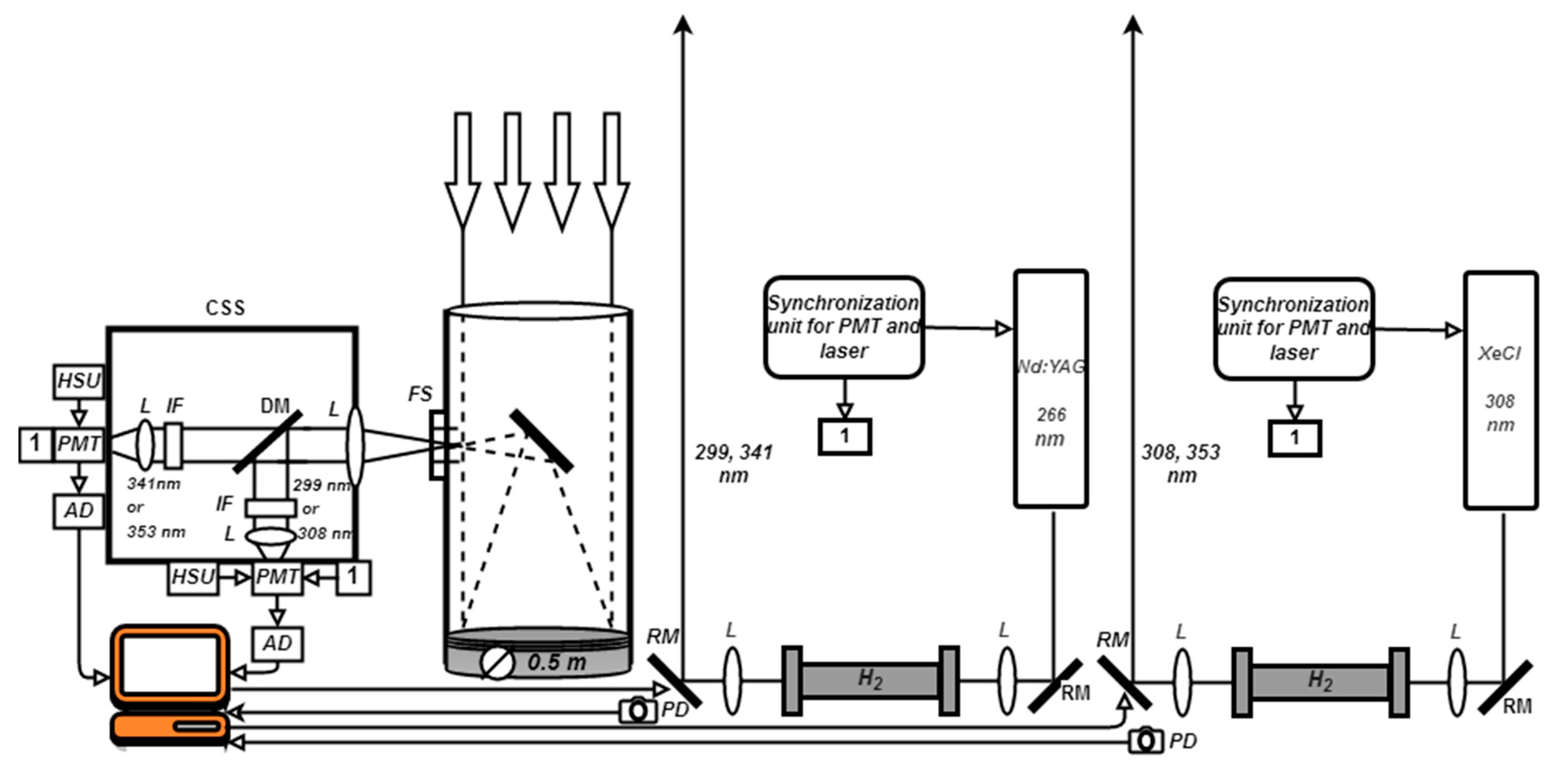
2.1. SLS Ozone Lidar Complex

In order to expand the possibilities of studying the characteristics of OVD in the upper troposphere–stratosphere, especially in the region of localization of the ozone layer, and control its seasonal variations, the lidar was upgraded and put into operation in the routine measurement mode in the altitude range ≈(5–45) km at wavelengths of 299/341 and 308/353 nm. The alternate lidar complex sounding of the ozonosphere at 299/341 and 308/353 nm wavelength pairs makes it possible to cover the altitude range from ≈5 to ≈45 km with the most successful measurements. Figure 1 shows the block diagram of the lidar complex [16].

Main specifications of laser sources and optical detecting elements of the lidar system are given below.

Transmitter	Nd:YAG	XeCl
Sounding wavelength λ, nm	299 341	308 353
Pulse energy, mJ (corresponding to λ)	25 20	100 50
Pulse frequency, Hz (corresponding to λ)	15	100
Beam divergence, mrad	0.1–0.3	0.1–0.3
Pulse duration, ns	5–6	25–27
Receiver
Mirror diameter, m	0.5
Focal length, m	1.5

Due to the lack of high-precision data of OVD measurements for Tomsk, the results of sensing MetOp satellites for the troposphere and Aura for the stratosphere were used. We compare the lidar measurement results with the results from MLS mounted onboard the Aura satellite [22] and with data from IASI mounted onboard the MetOp meteorological satellite [23]. The paper presents the data of lidar and satellite measurements carried out simultaneously or with a small difference in time over several hours.

2.2. MLS/Aura

The MLS microwave radiometer operates onboard the American scientific-research satellite Aura, which measures such atmospheric constituents as BrO, CH₃Cl, CO, ClO, HCl, HNO₃, HO₂, N₂O, O₃, etc., as well as air temperature and humidity profiles in the stratosphere within the NASA (National Aeronautics and Space Administration) Earth Observing System Program. Standard ozone data products (240-GHz radiation) are used, retrieved with the use of free-access data processing algorithm Version 4.2 [24]. MLS data are freely accessible on the NASA website [25]. The information makes it possible to compare satellite data with the SLS lidar sounding results.

2.3. IASI/MetOp

The IASI interferometer is mounted onboard the meteorological satellite of the European Space Agency (MetOp), which measures such atmospheric constituents as CO₂, CH₄, N₂O, CO, O₃, and HNO₃, as well as air temperature and humidity profiles in the troposphere and lower stratosphere within the European Polar System Program in the near-real-time mode. IASI provides high-radiometric quality spectra with a resolution of 0.5 cm⁻¹ in the range from 625 to 2760 cm⁻¹ [26]. Ozone profiling from satellite sounding data is performed in the range 1025–1075 cm⁻¹. IASI data are received with the help of a 2.4 XLB satellite information receiving station (Orbital Systems, USA), which has been operating at IAO SB RAS since 2011. We receive IASI ozone profiles from the IAO SB RAS satellite data receiving station with spatial resolution from ≈150 m in the surface layer to several kilometers in the stratosphere and higher (from ≈150 m to ≈80 km) [27].

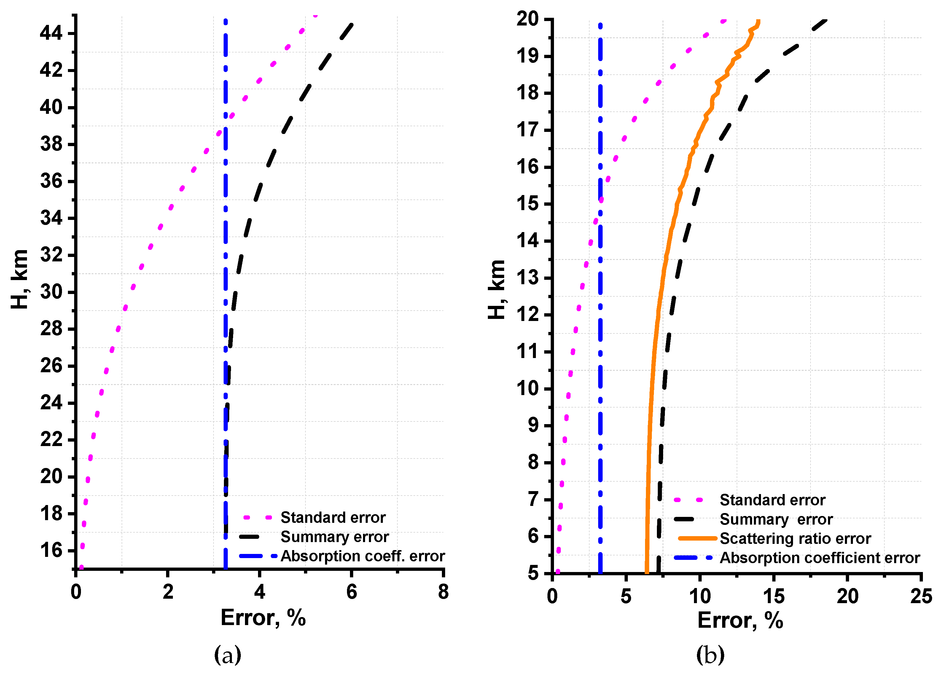
3. Measurement Technique and Analysis of Errors

The differential absorption lidar technique (DIAL) is the most sensitive among the techniques used to determine the spatial distribution of the concentration of any atmospheric gas, including ozone. This technique is intended for retrieving the lidar OVD profiles, taking into account the temperature and aerosol corrections, and is based on the equation [28,29]:

$$n\left(H\right)=\frac{1}{2\cdot \Delta k\left(H,T\right)}\times \left\{\frac{d}{dH}\ln \left[\frac{N_{off}\left(H\right)}{N_{on}\left(H\right)}\right]-\frac{d}{dH}\ln \left[\frac{{\beta }_{off}^a\left(H\right)+{\beta }_{off}^m\left(H\right)}{{\beta }_{on}^a\left(H\right)+{\beta }_{on}^m\left(H\right)}\right]-2\cdot \left[{\alpha }_{off}^a\left(H\right)-{\alpha }_{on}^a\left(H\right)\right]-2\cdot \left[{\alpha }_{off}^m\left(H\right)-{\alpha }_{on}^m\left(H\right)\right]\right\}$$

(1)

where N(H) is the return signal recorded at the corresponding wavelengths (on absorption line and off the absorption line); α^α is the aerosol scattering coefficient; α^m is the molecular scattering coefficient; β^m(H) is the molecular backscattering coefficient; β^α(H) is the aerosol backscattering coefficient; ∆k(H,T) is the absorption cross section differential; and n(H) is the ozone concentration.

Actual variations in atmospheric temperature can significantly change the a priori calculated ozone absorption cross section, which results in systematic errors in the OVD profile retrieval. Therefore, the correction to the temperature dependence is advisable in the OVD retrieval Algorithm (1). The technique suggested uses the temperature dependence of the ozone absorption cross section, which has been derived from the latest experimental and calculation data from [30,31].

At high aerosol content of the atmosphere, the aerosol backscattering is several times stronger than the molecular one, which, with unaccounted scattering and attenuating properties of the atmosphere at the sounding wavelengths, significantly distorts the ozone profile retrieved [32].

To compare the satellite and lidar data, it is important to take into account the vertical distribution of their errors. The total error of OVD retrieval from lidar measurements is calculated as

$$E_{sum}{}^2=e_1^2+e_2^2+e_3^2,$$

(2)

where e₁ is the cross section error; e₂ is the standard error of lidar measurements in the photon counting mode; e₃ is the error of scattering ratio retrieval. The absorption cross section uncertainty, which is 3.26%, was calculated as square root of the sum of squares of systematic and random uncertainties, obtained in work [30].

The standard lidar error in the photon counting mode is given as

$$e_2^2=0.25\times {\left(\frac{1}{N_{on}\left(H\right)}+\frac{1}{N_{off}\left(H\right)}\right)}_{}$$

(3)

The scattering ratio retrieval error is given by

$$e_3^2=\frac{N_{off}\left(H\right)}{{\left(N_{off}\left(H\right)-N_{noise}\left(H\right)\right)}^2}+\frac{N_{off}\left(H_{calib}\right)}{{\left(N_{off}\left(H_{calib}\right)-N_{noise}\left(H_{calib}\right)\right)}^2}+K,$$

(4)

where H_calib is the calibration altitude; N_noise is noise signal; K = 3 × (0.01)² is the constant caused by the processing technique suggested by El’nikov et al. [33].

Figure 2 shows the OVD measurement errors of the lidar complex in the upper troposphere–stratosphere. The ozone concentration error (2) is within 6% for the 15–45 km altitude range (stratospheric OVD at 308/353 nm) and 7.2–18.5% for the altitude range 5–20 km (OVD in the upper troposphere–lower stratosphere at 299/341 nm). IASI errors reach values of 30% in the upper troposphere–lower stratosphere. MLS errors reach values of 8% in the stratosphere. Thus, alternating sounding of ozone with the lidar complex at wavelength pairs 299/341 and 308/353 nm allows covering the altitude range from ≈5 to ≈45 km in the most successful measurements. During the observed period, the stratosphere over the SLS was in an unperturbed state; therefore, aerosol correction was not used in retrieving the OVD of the stratosphere. All measurements were selected for the conditions of the unperturbed troposphere (no clouds and no anomalous aerosol loading). All ozone profiles retrieved were subject to the procedure of aerosol correction.

4. Measurement results and discussion

On the basis of lidar measurements for 2018, average OVD profiles have been retrieved; they combine the lidar control of the stratosphere and the upper troposphere–lower stratosphere. Figure 3 shows the result of superposition of the ozone profiles retrieved from the lidar data for 2018, in comparison with the Krueger model [34].

The mid-latitude Krueger model, obtained from the average annual ozone probe, satellite rocket measurements at an altitude of 74 km, was used for comparison with the OVD data from satellites and lidar.

During 2018, 81 measurements of stratospheric OVD were made; 79 measurements were in the upper troposphere–lower stratosphere. The 25 measurements are given in this work. Using the above technique, we retrieved ozone profiles for the stratosphere and upper troposphere–lower stratosphere. They are compared with IASI and MLS profiles. The coordinates and times of lidar and satellite sounding sessions are given in

Table 2. Coordinates and time of MLS/Aura and lidar sounding used for the comparison of OVD in 2018.

Date	SLS (56.5° N, 85.0°E)	Distance between SLS and Aura, km	MLS/Aura
	GMT		GMT	Coordinates (° N, ° E)
January 13	12:25–13:04	437	07:07	60.43, 84.56
January 22	12:12–12:42	446	07:01	60.43, 86.10
January 23	13:13–13:43	681	21:14	51.74, 78.10
January 24	12:12–12:42	505	06:49	60.43, 89.20
January 26	13:19–13:49	613	06:36	60.43, 92.29
January 30	12:45–13:15	532	07:49	54.65, 77.13
January 31	13:15–13:45	350	06:55	58.99, 88.61
February 5	12:34–13:05	218	07:12	54.65, 86.41
February 12	13:42–14:12	101	20:48	56.10, 86.47
February 13	12:49–13:19	528	21:30	58.99, 77.38
February 21	14:01–14:31	249	20:42	54.65, 87.28
February 26	14:31–15:01	106	21:00	56.10, 83.40
March 5	13:29–13:59	198	21:06	56.10, 81.86
March 12	14:40–15:10	328	21:12	59.00, 82.01
March 13	13:46–14:16	430	06:48	56.11, 91.91
June 9	18:07–18:37	388	21:18	56.11, 78.74
September 27	14:12–14:42	386	07:47	51.74, 77.13
September 28	14:19–14:49	631	20:24	51.74, 90.50
October 15	13:48–14:18	438	07:35	53.20, 81.04
October 26	14:16–14:46	491	07:19	60.44, 81.58
November 16	12:29–12:59	351	07:36	54.66, 80.31
December 3	12:27–12:57	491	06:42	59.00, 91.78
December 4	11:13–11:43	145	07:24	56.11, 82.65
December 10	11:29–11:59	428	06:48	56.11, 91.92
December 26	11:14–11:44	426	20:17	56.11, 91.92

and

Table 3. Coordinates and time of IASI/MetOp and lidar sounding used for the comparison of OVD in 2018.

Date	SLS (56.5° N, 85.0°E)	IASI/MetOp
	GMT	GMT	Coordinates (° N, ° E)
January 13	13:28 – 14:02	13:53	56.47, 85.04
January 22	12:58 – 13:32	14:08	56.47, 85.04
January 23	12:15 – 12:49	14:29	56.47, 85.04
January 24	13:04 – 13:38	14:08	56.47, 85.04
January 26	12:25 – 12:59	14:23	56.47, 85.04
January 30	13:27 – 14:01	13:44	56.47, 85.04
January 31	12:26 – 13:00	14:20	56.47, 85.04
February 5	13:14 – 13:48	14:17	56.47, 85.04
February 12	12:50 – 13:24	14:14	56.47, 85.04
February 13	13:25 – 13:59	13:56	56.47, 85.04
February 21	13:10 – 13:44	15:26	56.47, 85.04
February 26	13:44 – 14:18	14:26	56.47, 85.04
March 5	14:14 – 14:48	13:41	56.47, 85.04
March 12	13:49 – 14:23	13:53	56.47, 85.04
March 13	14:28 – 15:02	14:14	56.47, 85.04
June 9	18:50 – 19:24	15:11	56.47, 85.04
September 27	14:56 – 15:30	15:14	56.47, 85.04
September 28	15:01 – 15:35	14:53	56.47, 85.04
October 15	12:58 – 13:32	14:02	56.47, 85.04
October 26	13:10 – 13:44	14:11	56.47, 85.04
November 16	13:15 – 13:49	13:35	56.47, 85.04
December 3	11:39 – 12:13	13:47	56.47, 85.04
December 4	11:57 – 12:31	14:02	56.47, 85.04
December 10	12:13 – 12:47	13:39	56.47, 85.04
December 26	12:00 – 12:40	14:11	56.47, 85.04

. The lidar measurements over Tomsk were carried out at the evening and night hours under clear sky conditions. The distance between the SLS and the MetOp satellite is 4.48 km (Table 3).

The selection was performed for satellite observations closest in time. The distance is not large between MetOp subsatellite points, whereas Aura data are obtained with a large spatial separation. However, for studies of the stratosphere—which is more static in character as compared to the troposphere, provided that no global volcanic effect on the ozonosphere is recorded—it is sufficient to select Aura measurements in time. Temporal selection of Aura data was carried out between two outermost measurement sets. First measurements were obtained at approximately ≈07:00 GMT and the second at ≈21:00 GMT; so, considering that lidar measurements are usually performed at 12:00–14:00 GMT, we had little to choose from because time difference is ≈7 h. Sometimes, satellite measurements at ≈07:00 GMT or ≈21:00 GMT are altogether absent. Therefore, the nearest measurements were chosen from the set available.

The deviations are due to the difference between the spatial resolutions of the lidar and Aura (100 m and ≥1.3 km, respectively); hence, the number of points that form the OVD is larger for the lidar, which also affects the behavior of the OVD profile retrieved. The measurements are reduced to the common altitude range 16–38 km for the convenience of comparison.

Figure 4a shows that Aura overestimates the ozone concentrations as compared to the lidar in the range from 22 to 38 km throughout the measurement period.

The following conclusions can be drawn from the analysis of the natural data on stratospheric OVD in the period under study (Figure 4). A small difference between the ozone concentration profiles (Figure 5a,b) measured by the lidar and Aura is observed at the bottom and top edges of the altitude range. As a result, the mean difference (lidar – Aura) or the deviation over all measurement days in ozone concentrations varies from −0.47 × 10¹² mol. × cm⁻³ at an altitude of 29 km to −0.15 × 10¹² mol. × cm⁻³ at 17 km (Figure 4b). The maximum deviation over all profiles is from −0.09 × 10¹² mol. × cm⁻³ at 32.1 km to 1.46 × 10¹² mol. × cm⁻³ at 16 km. The minimum deviation over all profiles also varies, from −1.8 × 10¹² mol. × cm⁻³ at 16 km to −0.48 × 10¹² mol. × cm⁻³ at 37 km.

Ozone has a pronounced annual behavior; therefore, to find the relative errors of its measurements by MLS/Aura, the concentration difference has been normalized to the lidar values: 100 × (lidar – Aura)/lidar. These data are shown in Figure 4c; one can see that the average relative difference is negative in the altitude range 16–38 km and attains −49.81% at 38 km.

The maximal relative difference varies from −4.26% to 45.27% at altitudes of 32.5 km and 38 km, respectively. The minimal relative difference over all profiles in these altitude ranges varies from −200.91% to −19.44% at altitudes of 37.9 km and 19.7 km, respectively. At an altitude of 16 km, the relative difference varies between minimum and maximum of −58.94% and 28.81%; and at 38 km, within −200.87% and 45.27%.

Thus, the comparison shows that the absolute differences in ozone concentration measured with the lidar and Aura/MLS can vary from −1.8×10¹² to 1.46×10¹² mol. × cm⁻³. Taking into account the minimum and maximum of the relative difference, we can conclude that it varies in the range from −200.87 to +45.27%.

SLS lidar ozone profiles and OVD from MetOp data (Figure 5) are reduced to the common altitude range 6–18 km for the convenience of comparison of all profiles.

It can be seen from Figure 5a that the lidar overestimates the ozone concentrations in comparison with MetOp in the range from 12 to 18 km throughout the period of observations.

We can draw the following conclusions from the analysis of the data on OVD in the upper troposphere–lower stratosphere for the period under study shown in Figure 5. The difference between the lidar and MetOp concentration profiles (Figure 5a,b) increases with altitude. As a result, the average difference (lidar−MetOp) or the deviation over all measurement days in ozone concentrations varies from −0.01 × 10¹² mol.× cm⁻³ at an altitude of 6.6 km to 1.99 × 10¹² mol. × cm⁻³ at 18 km (Figure 5b). The maximal deviation over all profiles is from 0.35 × 10¹² mol. × cm⁻³ at an altitude of 6.6 km to 3.78 × 10¹² mol. × cm⁻³ at 18 km. The minimal deviation also varies from −0.45 × 10¹² mol. × cm⁻³ at 6.6 km to 0.99 × 10¹² mol. × cm⁻³ at 16.8 km.

Ozone shows a pronounced annual behavior; therefore, to find the relative errors in its measurements with IASI/MetOp, the concentration difference has been normalized to the lidar values: 100 × (lidar − MetOp)/lidar. These data are shown in Figure 5c; it is seen that the average relative difference is positive in the altitude ranges 6 and 7.4–18 km, where it attains 43.68% at 16.8 km, and is negative in the altitude range 6–7.3 km, where it attains −43.86% at 6.2 km.

The maximal relative difference varies from 41.35% to 80.73% at altitudes of 6.6 and 6 km, respectively. The minimal relative difference over all the profiles is −300.08% at 6.1 km and attains 26.56% at 15.3 km. This minimum of the relative difference is due to measurements (January 13, 22, 2018, etc.), when the satellite values were much higher than the lidar data. Therefore, such a loop is observed at altitudes from 6 to 8 km in Figure 5c. At an altitude of 18 km, the relative difference varies between the minimum and maximum, from 9.67% to 63.34%, and at 6 km, from −300.14% to 80.73%.

Thus, the comparison shows that the absolute differences in ozone concentration measured with the lidar and MetOp can vary from −0.45 × 10¹² to 3.78 10¹² mol.×cm⁻³. Taking into account the minimum and maximum of the relative difference, its variations can be found to be in the range −300.08%–+80.73%.

Thus, the comparison shows that the absolute differences in ozone concentration measured with the lidar and MetOp can vary from −0.36 × 10¹² to 2.35 × 10¹² mol. × cm⁻³. Taking into account the minimum and maximum of the relative difference, its variations can be found to be in the range −261.53%–+80.73%.

We extracted two seasonal periods from annual measurements of ozone vertical distribution by lidar and satellite. These are winter–spring (November–April) and summer–fall (May–October), used in Figure 6 and Figure 7 for stratospheric comparisons and in Figure 8 and Figure 9 for tropospheric comparisons. A characteristic feature of the winter-fall period is that larger ozone concentrations were observed at altitudes of the stratosphere and upper troposphere as compared to the second period. This is due to meridional transport of cold air masses form the North Pole in winter period. The comparisons, obtained for the study periods, are numerically described in

Table 4. Comparison of lidar and Aura satellite data for two seasons: winter-spring and summer-fall.

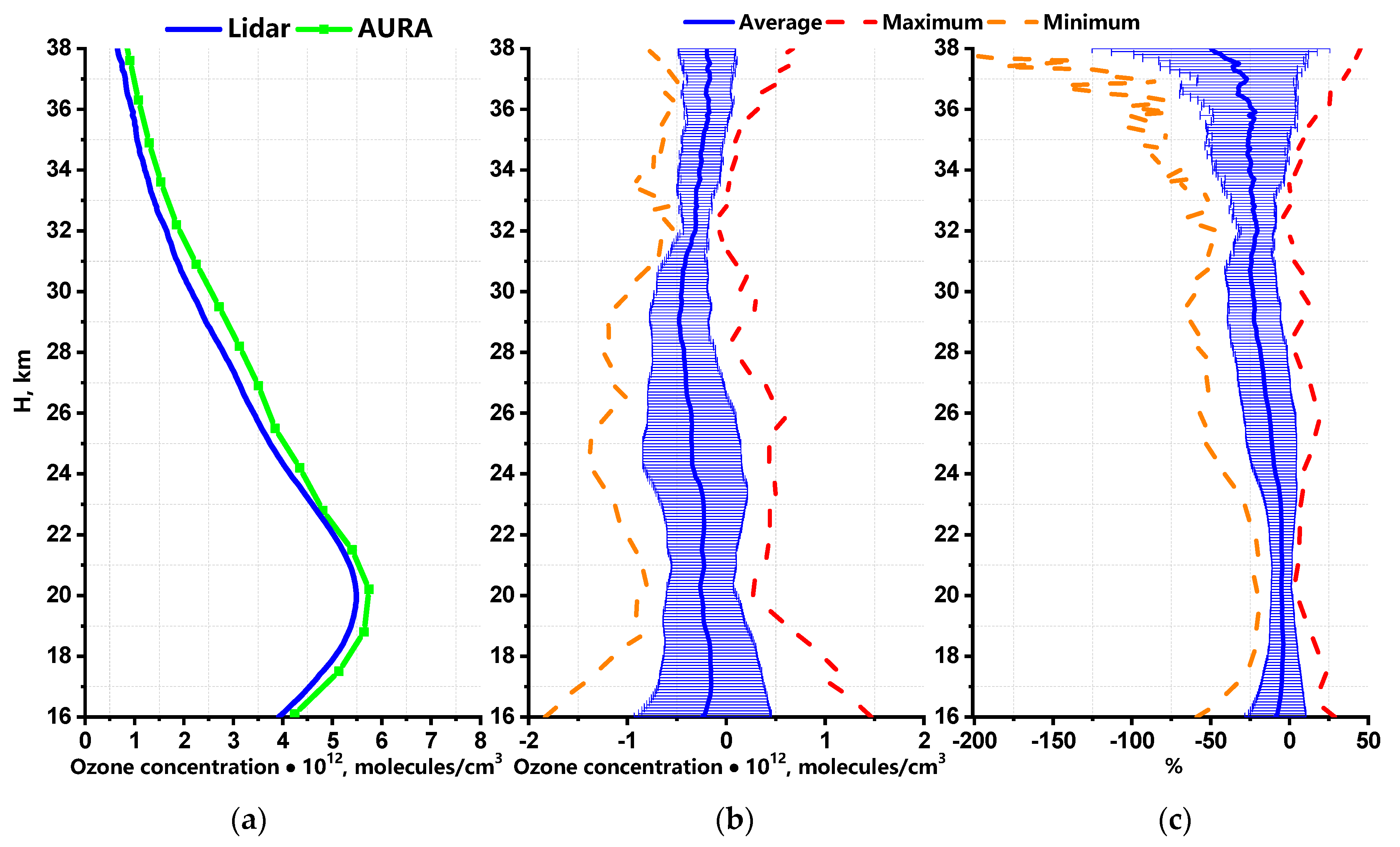
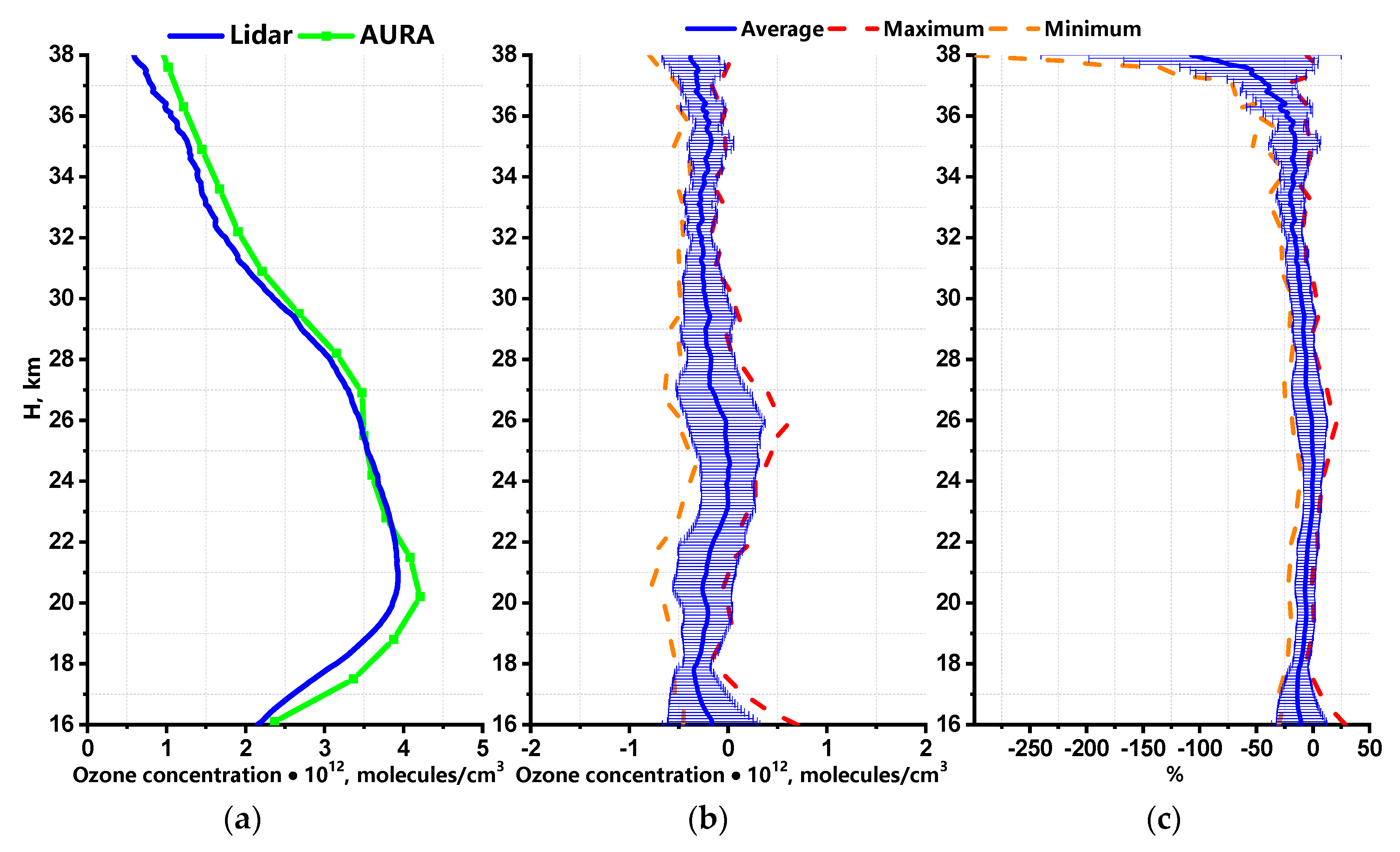
Stratosphere Lidar and MLS (16–38 km)
Winter–Spring
	Lidar − MLS × 1012 molecules/cm3	100 ×(Lidar − MLS)/Lidar %
Minimum	from −1.83 at 16 km to −0.41 at 37.1 km	from −182.65 at 37.4 km to −14.96 at 18.7 km
Maximum	from −0.09 at 32.1 km to 1.46 at 16 km	from −4.26 at 32.5 km to 45.27 at 38 km
Average	from −0.54 at 29.1 km to −0.1 at 17.5 km	from −35.45 at 37.9 km to −2.34 at 17.9 km
Summer–Fall
Minimum	from −1.83 at 16 km to −0.41 at 37.1 km	from −299.87 at 38 km to −10.67 at 24.5 km
Maximum	from −0.18 at 37.1 km to 0.7 at 16 km	from −21.63 at 36.8 km to 28.81 at 16 km
Average	from −0.38 at 37.9 km to −0.01 at 24.5 km	from −107.64 at 38 km to 0.57 at 24.6 km

and

Table 5. Comparison of lidar and IASI satellite data for two seasons: winter-spring and summer-fall.

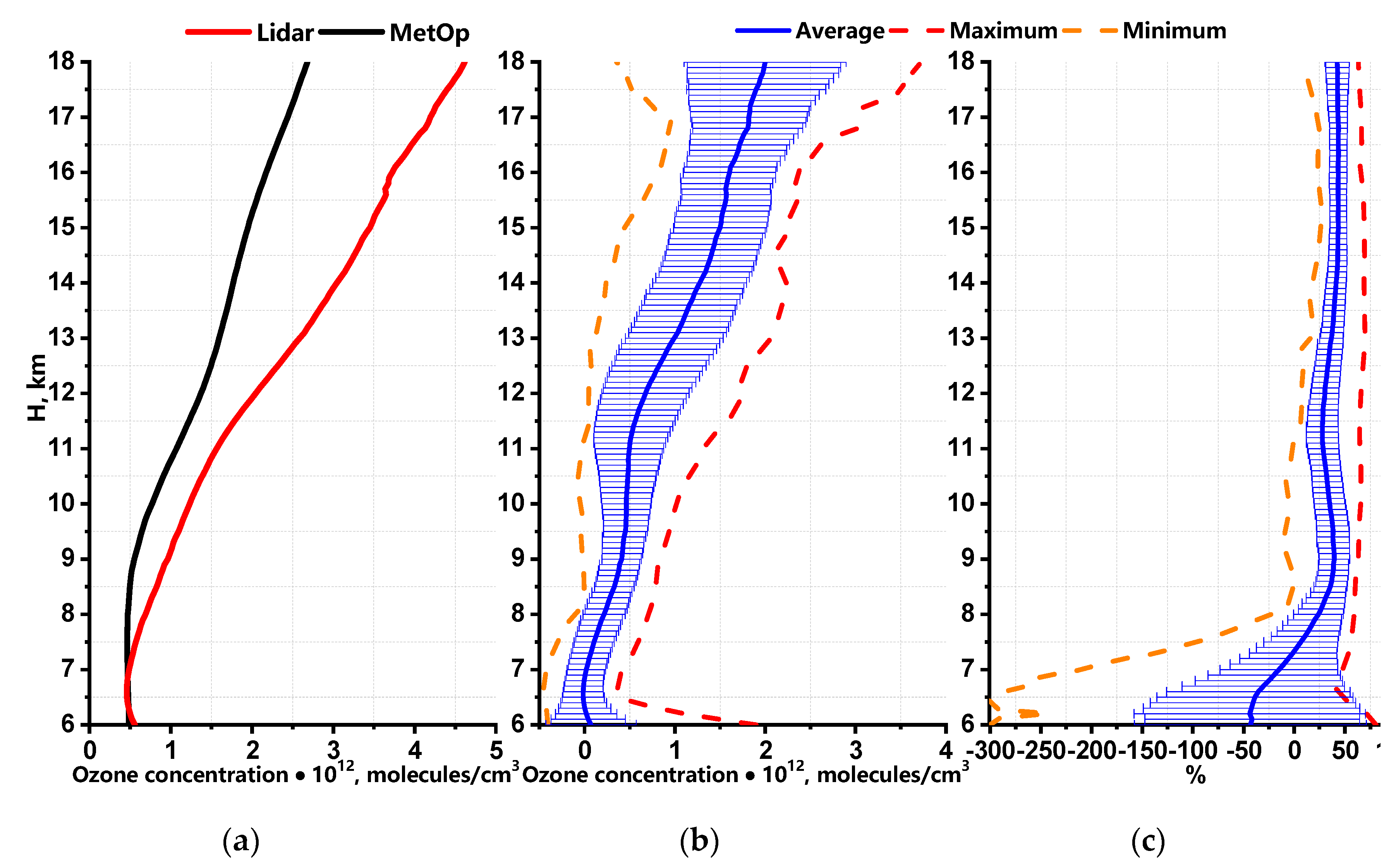
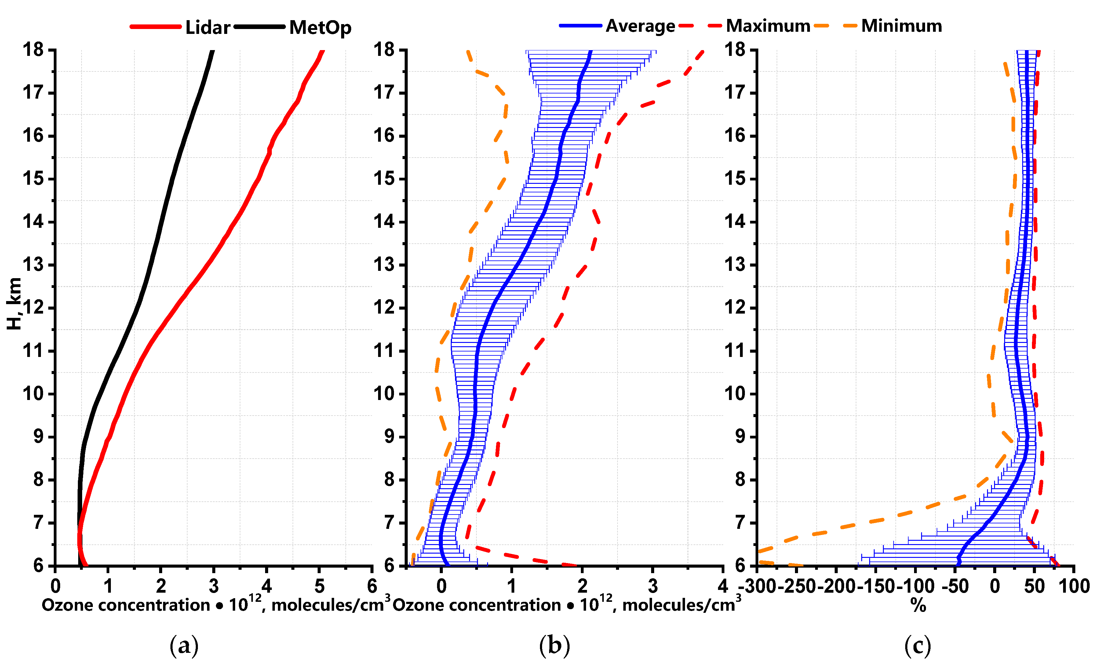
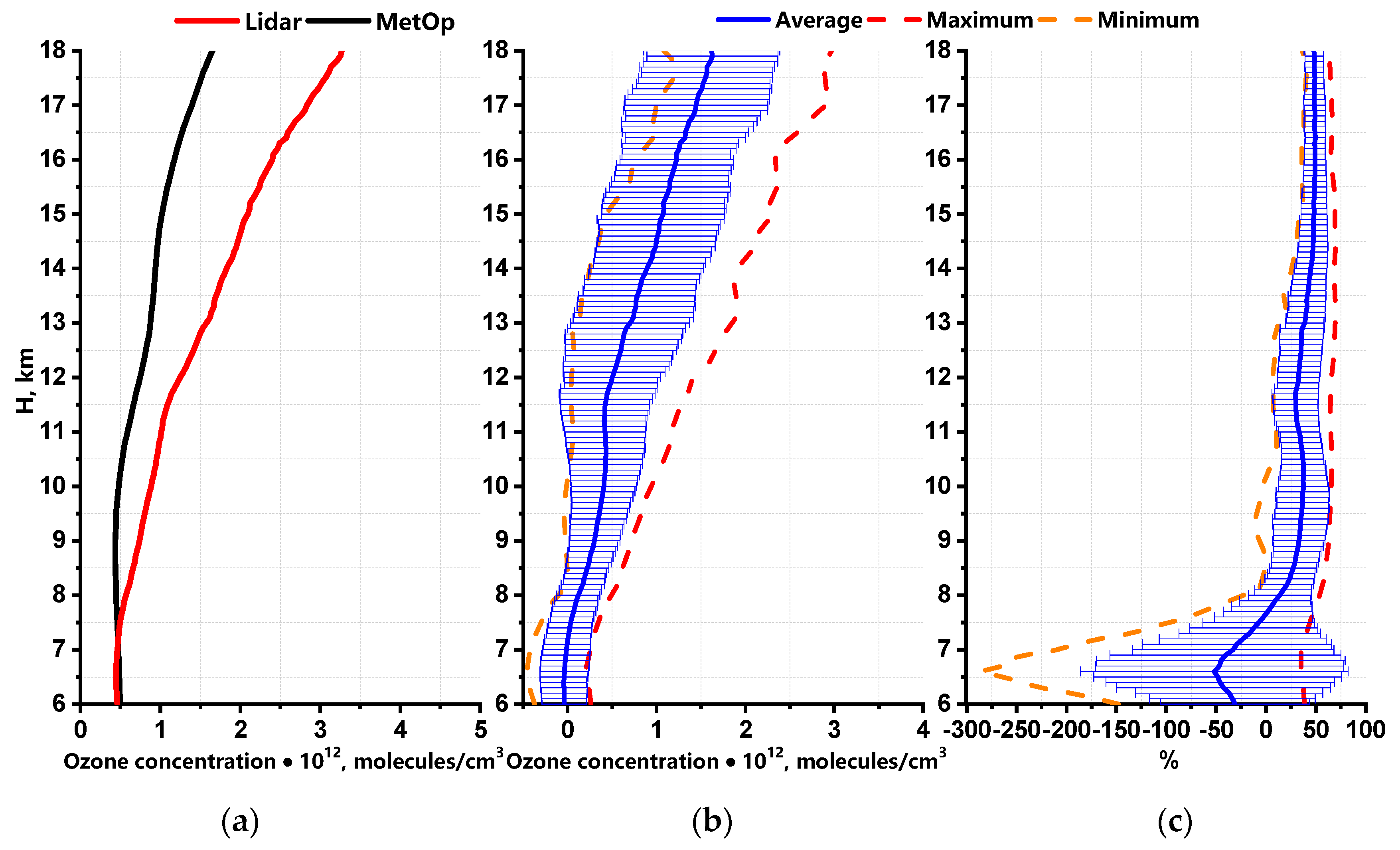
Troposphere Lidar and IASI (6–18 km)
Winter–Spring
	Lidar − IASI × 1012 molecules/cm3	100 ×(Lidar − IASI)/Lidar %
Minimum	from −0.4 at 6 km to 0.99 at 16.8 km	from −299 at 6.1 km to 26.56 at 15.3 km
Maximum	from 0.35 at 6.6 km to 3.78 at 18 km	from 41.35 at 6.6 km to 80.73 at 6 km
Average	from −0.01 at 6.6 km to 2.12 at 18 km	from −46.92 at 6 km to 42.07 at 15 km
Summer–Fall
Minimum	from −0.45 at 6.6 km to 1.19 at 17.6 km	from −287.03 at 6.6 km to 40.72 at 17.5 km
Maximum	from 0.20 at 6.6 km to 2.97 at 18 km	from −34.55 at 6.9 km to 69.71 at 13.1 km
Average	from −0.04 at 6.4 km to 1.62 at 17.9 km	from −51.8 at 6.6 km to 49.6 at 16.4 km

.

Figure 6a and Figure 7a show a good agreement between lidar and Aura data in the stratosphere.

Figure 10 shows some common OVDs that combine (stitched ozone profile) the lidar control of the stratosphere and the upper troposphere–lower stratosphere into a common OVD curve. Such a comprehensive approach to OVD measurements allows more comprehensive lidar monitoring of stratospheric-tropospheric air mass exchange processes.

5. Conclusion

Thus, a lidar complex was used to measure OVD in the upper troposphere–stratosphere, in the altitude range ≈(5–45) km at wavelengths of 299/341 nm and 308/353 nm.

The comparison shows that the absolute differences in ozone concentration measured with the lidar and IASI/MetOp can vary from −0.36 × 10¹² to 2.35 × 10¹² mol. × cm⁻³, and the difference between lidar and MLS/Aura can vary from −1.8 × 10¹² to 1.46 × 10¹² mol. × cm⁻³. Taking into account the minimum and maximum of the relative difference, for lidar and IASI/MetOp variations they are found to be in the range −261.53%–+80.73%, and for lidar and MLS/Aura in the range −200.87–+45.27%.

The retrieved lidar OVD profiles in the upper troposphere–stratosphere in comparison with MLS/Aura and IASI/MetOp profiles for 2018, as well as the stitched OVD profile in the upper troposphere–stratosphere in comparison with the mid-latitude Krueger model, confirm the prospects of using the pairs of ozone sounding wavelengths 299/341 and 308/353 nm in the altitude range 6–38 km.

References

1. Weitkamp, C. Lidar: Range Resolved Optical Remote Sensing of the Atmosphere; Springer: Berlin/Heidelberg, Germany, 2005; pp. 1–18. [Google Scholar]
2. Park, C.B.; Nakane, H.; Sugimoto, N.; Matsui, I.; Sasano, Y.; Fujinuma, Y.; Ikeuchi, I.; Kurokawa, J.-I.; Furuhashi, N. Algorithm improvement and validation of National Institute for Environmental Studies ozone differential absorption lidar at the Tsukuba Network for Detection of Stratospheric Change complementary station. Appl. Opt. 2006, 45, 3561–3576. [Google Scholar] [CrossRef] [PubMed]
3. Nakazato, M.; Nagai, T.; Sakai, T.; Hirose, Y. Tropospheric ozone differential-absorption lidar using stimulated Raman scattering in carbon dioxide. Appl. Opt. 2007, 46, 2269–2279. [Google Scholar] [CrossRef] [PubMed]
4. Godin, S.; Bergeret, V.; Bekki, S.; David, C.; Mégie, G. Study of the interannual ozone loss and the permeability of the Antarctic Polar Vortex from long-term aerosol and ozone lidar measurements in Dumont d’Urville (66.4°, 140° S). J. Geophys. Res. 2001, 106, 1311–1330. [Google Scholar] [CrossRef]
5. Gaudel, A.; Ancellet, G.; Godin-Beekmann, S. Analysis of 20 years of tropospheric ozone vertical profiles by lidar and ECC at Observatoire de Haute Provence (OHP) at 44 N, 6.7 E. Atmos. Environ. 2015, 113, 78–89. [Google Scholar] [CrossRef]
6. Hu, S.; Hu, H.; Wu, Y.; Zhou, J.; Qi, F.; Yue, G. Atmospheric ozone measured by differential absorptionlidar over Hefei. Proc. SPIE 2003, 466591. [Google Scholar] [CrossRef]
7. Liu, X.; Zhang, Y.; Hu, H.; Tan, K.; Tao, Z.; Shao, S.; Cao, K.; Fang, X.; Yu, S. Mobile lidar for measurements of SO2 and O3 in the low troposphere. Proc. SPIE 2005. [Google Scholar] [CrossRef]
8. McDermid, I.S.; Godin, S.M.; Lindquist, L.O. Ground-based laser DIAL system for long-term measurements of stratospheric ozone. Appl. Opt. 1990, 29, 3603–3612. [Google Scholar] [CrossRef]
9. McDermid, I.S.; Beyerle, G.; Haner, D.A.; Leblanc, T. Redesign and improved performance of the tropospheric ozone lidar at the Jet Propulsion Laboratory Table Mountain Facility. Appl. Opt. 2002, 41, 7550–7555. [Google Scholar] [CrossRef]
10. Steinbrecht, W.; McGee, T.J.; Twigg, L.W.; Claude, H.; Schönenborn, F.; Sumnicht, G.K.; Silbert, D. Intercomparison of stratospheric ozone and temperature profiles during the October 2005 Hohenpeißenberg Ozone Profiling Experiment (HOPE). Atmos. Meas. Tech. 2009, 2, 125–145. [Google Scholar] [CrossRef] [Green Version]
11. Sullivan, J.T.; McGee, T.J.; Sumnicht, G.K.; Twigg, L.W.; Hoff, R.M. A mobile differential absorption lidar to measure sub-hourly fluctuation of tropospheric ozone profiles in the Baltimore–Washington, D.C. region. Atmos. Meas. Tech. 2014, 7, 3529–3548. [Google Scholar] [CrossRef] [Green Version]
12. Pavlov, A.N.; Stolyarchuk, S.Y.; Shmirko, K.A.; Bukin, O.A. Lidar Measurements of Variability of the Vertical Ozone Distribution Caused by the Stratosphere–Troposphere Exchange in the Far East Region. Atmos. Ocean. Opt. 2013, 26, 126–134. [Google Scholar] [CrossRef]
13. Burlakov, V.D.; Dolgii, S.I.; Nevzorov, A.V. Modification of the measuring complex at the Siberian Lidar Station. Atmos. Ocean. Opt. 2004, 17, 756–762. [Google Scholar]
14. Dolgii, S.I.; Nevzorov, A.A.; Nevzorov, A.V.; Romanovskii, O.A.; Makeev, A.P.; Kharchenko, O.V. Lidar Complex for Measurement of Vertical Ozone Distribution in the Upper Troposphere–Stratosphere. Atmos. Ocean. Opt. 2018, 31, 1–7. [Google Scholar] [CrossRef]
15. Fang, X.; Li, T.; Ban, C.; Wu, Z.; Li, J.; Li, F.; Cen, Y.; Tian, B. A mobile differential absorption lidar for simultaneous observations of tropospheric and stratospheric ozone over Tibet. Opt. Express 2019, 27, 4126–4139. [Google Scholar] [CrossRef] [PubMed]
16. Network for the Detection of Atmospheric Composition Change. Information of Lidar Stations. Available online: http://www.ndaccdemo.org/ (accessed on 28 December 2019).
17. Dolgii, S.I.; Nevzorov, A.A.; Nevzorov, A.V.; Romanovskii, O.A.; Kharchenko, O.V. Intercomparison of Ozone Vertical Profile Measurements by Differential Absorption Lidar and IASI/MetOp Satellite in the Upper Troposphere–Lower Stratosphere. Remote Sens. 2017, 9, 447. [Google Scholar] [CrossRef] [Green Version]
18. Jiang, Y.B.; Froidevaux, L.; Lambert, A.; Livesey, N.J.; Read, W.G.; Waters, J.W.; Bojkov, B.; Leblanc, T.; McDermid, I.S.; Godin-Beekmann, S.; et al. Validation of Aura Microwave Limb Sounder Ozone by ozonesonde and lidar measurements. J. Geophys. Res. 2007, 112. [Google Scholar] [CrossRef]
19. Kirgis, G.; Leblanc, T.; McDermid, I.S.; Walsh, T.D. Stratospheric ozone interannual variability (1995–2011) as observed by lidar and satellite at Mauna Loa Observatory, HI and Table Mountain Facility, CA. Atmos. Chem. Phys. 2013, 13, 5033–5047. [Google Scholar] [CrossRef] [Green Version]
20. Nair, P.J.; Godin–Beekmann, S.; Froidevaux, L.; Flynn, L.E.; Zawodny, J.M.; Russell III, J.M.; Pazmiño, A.; Ancellet, G.; Steinbrecht, W.; Claude, H.; et al. Relative drifts and stability of satellite and ground-based stratospheric ozone profiles at NDACC lidar stations. Atmos. Meas. Tech. 2012, 5, 1301–1318. [Google Scholar] [CrossRef] [Green Version]
21. Gazeaux, J.; Clerbaux, C.; George, M.; Hadji-Lazaro, J.; Kuttippurath, J.; Coheur, P.-F.; Hurtmans, D.; Deshler, T.; Kovilakam, M.; Campbell, P.; et al. Intercomparison of polar ozone profiles by IASI/MetOp sounder with 2010 Concordiasi ozonesonde observations. Atmos. Meas. Tech. 2013, 6, 613–620. [Google Scholar] [CrossRef] [Green Version]
22. Waters, J.W.; Froidevaux, L.; Harwood, R.S.; Jarnot, R.F.; Pickett, H.M.; Read, W.G.; Siegel, P.H.; Cofield, R.E.; Filipiak, M.J.; Flower, D.A.; et al. The Earth Observing System Microwave Limb Sounder (EOS MLS) on the Aura Satellite. IEEE (TGRS) Trans. Geosci. Remote Sens. 2006, 44, 1075–1092. [Google Scholar] [CrossRef]
23. Clerbaux, C.; Boynard, A.; Clarisse, L.; George, M.; Hadji-Lazaro, J.; Herbin, H.; Hurtmans, D.; Pommier, M.; Razavi, A.; Turquety, S.; et al. Monitoring of atmospheric composition using the thermal infrared IASI/MetOp sounder. Atmos. Chem. Phys. 2009, 9, 6041–6054. [Google Scholar] [CrossRef] [Green Version]
24. NASA (National Aeronautics and Space Administration). Microwave Limb Sounder. The MLSO3 Product. Available online: https://mls.jpl.nasa.gov/products/o3_product.php (accessed on 28 October 2019).
25. NASA (National Aeronautics and Space Administration). MLS Ozone Data. Available online: https://avdc.gsfc.nasa.gov/pub/data/satellite/Aura/MLS/V04/L2GPOVP/O3/ (accessed on 28 October 2019).
26. August, T.; Klaes, D.; Schlüssel, P.; Hultberg, T.; Crapeau, M.; Arriaga, A.; O’Carroll, A.; Coppens, D.; Munro, R.; Calbet, X. IASI on Metop-A: Operational Level 2 retrievals after five years in orbit. J. Quant. Spectrosc. Radiat. Transf. 2012, 113, 1340–1371. [Google Scholar] [CrossRef]
27. Matvienko, G.G.; Belan, B.D.; Panchenko, M.V.; Romanovskii, O.A.; Sakerin, S.M.; Kabanov, D.M.; Turchinovich, S.A.; Turchinovich, Y.S.; Eremina, T.A.; Kozlov, V.S.; et al. Complex experiment on studying the microphysical, chemical, and optical properties of aerosol particles and estimating the contribution of atmospheric aerosol-to-earth radiation budget. Atmos. Meas. Tech. 2015, 8, 4507–4520. [Google Scholar] [CrossRef] [Green Version]
28. Measures, R.M. Laser Remote Sensing. Fundamentals and Applications; Reprint 1984 de Krieger Publishing Company: Malabar, FL, USA, 1992; pp. 237–280. [Google Scholar]
29. Burlakov, V.D.; Dolgii, S.I.; Nevzorov, A.A.; Nevzorov, A.V.; Romanovskii, O.A. Algorithm for Retrieval of Vertical Distribution of Ozone from DIAL Laser Remote Measurements. Opt. Mem. Neural Netw. (Inf. Opt.) 2015, 24, 295–302. [Google Scholar] [CrossRef]
30. Gorshelev, V.; Serdyuchenko, A.; Weber, M.; Chehade, W.; Burrows, J.P. High spectral resolution ozone absorption cross-sections–Part 1: Measurements, data analysis and comparison with previous measurements around 293 K. Atmos. Meas. Tech. 2014, 7, 609–624. [Google Scholar] [CrossRef] [Green Version]
31. Serdyuchenko, A.; Gorshelev, V.; Weber, M.; Chehade, W.; Burrows, J.P. High spectral resolution ozone absorption cross-sections-Part 2: Temperature dependence. Atmos. Meas. Tech. 2014, 7, 625–636. [Google Scholar] [CrossRef] [Green Version]
32. El’nikov, A.V.; Zuev, V.V. Bifrequency laser sounding of stratospheric ozone under conditions of high degree of aerosol loading. Atmos. Ocean. Opt. 1992, 5, 681–683. [Google Scholar]
33. El’nikov, A.V.; Marichev, V.N.; Shelevoi, K.D.; Shelefontyuk, D.I. Laser radar for sensing vertical stratification of atmospheric aerosol. Atmos. Ocean. Opt. 1988, 1, 117–123. [Google Scholar]
34. Krueger, A.J.; Minzner, R.A. Mid-latitude ozone model for the 1976 U.S. Standard Atmosphere. J. Geophys. Res. 1976, 81, 4477–4481. [Google Scholar] [CrossRef]
Figure 1. Block diagram of the ozone lidar complex: field stop (FS), cuvette of spectral selection with a photomultiplier (CSS), interference filter (IF), dichroic mirror (DM), amplifiers–discriminators (AD), high-voltage supply units (HSU), rotary mirrors (RM), lenses (L), photomultiplying tube (PMT), photodiodе (PD).
Atmosphere 11 00196 g001
Figure 2. Average measurement errors of ozone vertical distribution (OVD) for 2018: error in the (a) stratosphere and (b) upper troposphere–lower stratosphere.
Atmosphere 11 00196 g002
Figure 3. Average profile retrieved in the upper troposphere–stratosphere in 2018.
Atmosphere 11 00196 g003
Figure 4. Average OVDs and their differences: (a) average profiles; (b) differences between the lidar and Aura data, in absolute units; (c) relative differences 100 × (lidar – Aura)/lidar.
Atmosphere 11 00196 g004
Figure 5. Average OVDs and their differences: (a) average profiles; (b) differences between the lidar and MetOp data, in absolute units; (c) relative differences 100 × (lidar − MetOp)/lidar.
Atmosphere 11 00196 g005
Figure 6. Average OVDs for season of winter–spring and their differences: (a) average profiles; (b) differences between the lidar and Aura data, in absolute units; and (c) relative differences 100 × (lidar – Aura)/lidar.
Atmosphere 11 00196 g006
Figure 7. Average OVDs for season of summer–fall and their differences: (a) average profiles; (b) differences between the lidar and Aura data, in absolute units; and (c) relative differences 100 × (lidar – Aura)/lidar.
Atmosphere 11 00196 g007
Figure 8. Average OVDs for season of winter–spring and their differences: (a) average profiles; (b) differences between the lidar and MetOp data, in absolute units; and (c) relative differences 100 × (lidar – MetOp)/lidar.
Atmosphere 11 00196 g008
Figure 9. Average OVDs for season of summer–fall and their differences: (a) average profiles; (b) differences between the lidar and MetOp data, in absolute units; and (c) relative differences 100 × (lidar – MetOp)/lidar.
Atmosphere 11 00196 g009
Figure 10. Comparison of ozone vertical profiles in the upper troposphere–stratosphere with Aura and MetOp satellite data.
Atmosphere 11 00196 g010