Article

Inter-Comparison of Ensemble Forecasts for Low Level Wind Shear against Local Analyses Data over Jeju Area

1
Environmental Meteorology Research Division, National Institute of Meteorological Sciences, Seogwipo 63631, Jeju, Korea
2
Department of Applied Mathematics, Kongju National University, 56 Gongjudaehak-ro, Gongju-si 32588, Chungcheongnam-do, Gongju, Korea
3
Applied Meteorology Research Division, National Institute of Meteorological Sciences, Seogwipo 63631, Jeju, Korea
*
Author to whom correspondence should be addressed.
Submission received: 7 January 2020 / Revised: 10 February 2020 / Accepted: 11 February 2020 / Published: 13 February 2020
(This article belongs to the Section Meteorology)

Abstract

:
Ensemble verification of low-level wind shear (LLWS) is an important issue in airplane landing operations and management. In this study, we conducted an accuracy and reliability analysis using a rank histogram, Brier score, and reliability diagram to verify LLWS ensemble member forecasts based on grid points over the Jeju area of the Republic of Korea. Thirteen LLWS ensemble member forecasts derived from a limited area ensemble prediction system (LENS) were obtained between 1 July 2016 and 30 May 2018, and 3-h LLWS forecasts for lead times up to 72 h (three days) were issued twice a day at 0000 UTC (9 am local time) and 1200 UTC (9 pm local time). We found that LLWS ensemble forecasts have a weak negative bias in summer and autumn and a positive bias in the spring and winter; the forecasts also have under-dispersion for all seasons, which implies that the ensemble spread of an ensemble is smaller than that of the corresponding observations. Additionally, the reliability curve in the associated reliability diagram indicates an over-forecasting of LLWS events bias. The selection of a forecast probability threshold from the LLWS ensemble forecast was confirmed to be one of the most important factors for issuing a severe LLWS warning. A simple method to select a forecast probability threshold without economic factors was conducted. The results showed that the selection of threshold is more useful for issuing a severe LLWS warning than none being selected.

1. Introduction

Wind shear events are usually associated with atmospheric instabilities caused by convective activity, specifically gust fronts and microbursts (National Research Council 1983). These events were the most common weather factors in a total of 1740 weather-related accidents reported in the United States airports during the early 2000s [1]. Damage related to high-impact weather, including wind shear, is also continuously reported and resulted in 3010 flight delays and cancellations in Korea in 2017 [2].
Prediction of the low-level wind shear (LLWS) over the airports has been mostly focused on detection and early warning systems based on measurements from the low level windshear alert system (LLWAS) and terminal doppler weather radar (TDWR) [3,4]. Later, as the rapid development of numerical weather prediction (NWP) models and high-performance computing capabilities occurred, wind shear forecasts based on specific weather prediction models were increasingly found to provide reliable and useful warnings about wind hazards [5,6]. Nevertheless, forecasting such wind disturbances is still an ongoing area of development in the field of NWP systems.
It is more appropriate, then, to utilize numerical forecasting to provide information on the relative likelihood of possible weather events. Ensemble forecasts have been developed as a complementary tool for deterministic forecasts by adapting multi-model runs with different possible initial conditions [7,8,9]. Recently, it has become possible to resolve convection-scale turbulence using local-scale ensemble forecasts or downscaled forecasts from larger-scale ensemble prediction systems [10,11,12]. Ensemble-based weather forecasting has also been applied to aviation meteorology to predict the weather hazards affecting aircraft operation and has been presented as a better tool for describing wind disturbances and their likely positions [13,14]. Zhou et al. [15,16] applied the National Centers for Environmental Prediction (NCEP) 32-km operational ensemble system from the Short-Range Ensemble Forecast, to LLWS ensemble forecasts. They also suggested that the LLWS ensemble forecasts could perform better than traditional deterministic forecasts through bias correction of numerically quantified uncertainties. However, it is still challenging to use ensemble forecasts to ensure sufficient accuracy for hazardous wind prediction around the airport.
In this study, the Korea Meteorological Administration (KMA)’s operational ensemble forecasts from the limited area ensemble prediction system (LENS) are used to generate probabilistic forecasts for almost two years (from July 2016 to May 2018). Since the Jeju International Airport is the most frequent area of wind shear among all 13 international and domestic airports in ROK, we conducted a reliability analysis based on grid points over the Jeju area. The ensemble forecasts from the LENS, which is the local-scale operational ensemble models of the KMA, are verified with their corresponding analysis data generated from the KMA’s operational local-scale atmospheric numerical model. A Reliability analysis using a rank histogram [17,18] and the statistical consistency of the LLWS forecast probability using the Brier score [19,20] as well as reliability diagram [21] were utilized to evaluate the statistical consistency of the ensembles. Moreover, the mean absolute error (MAE), root mean square error (RMSE), and continuous ranked probability score (CRPS) were used to assess the prediction skill of the ensemble forecasts. The selection of a forecast probability threshold from the LLWS ensemble forecast is one of the most important factors for issuing a severe LLWS warning. Therefore, we also considered the selection of a forecast probability threshold when we use the probability information in forecasting LLWS. This paper presents preliminary results of the LLWS ensemble forecasts and provides general principles for ensemble forecast verification. Also, LLWS ensemble information analyzed from the LENS forecast output can be used to reduce the bias and spread of the ensemble system.
The rest of this paper is organized as follows: the LLWS ensemble forecasts used for analysis are described in Section 2. The reliability analysis of the LLWS ensemble and its corresponding analysis data, prediction skill of the ensembles, and statistical consistency of the LLWS forecast probability are indicated in Section 3. A simple method to select a forecast probability threshold and its results are also discussed in Section 3. Finally, conclusions are given in Section 4.

2. LLWS Ensemble Forecast

The LENS is based on the MOGREPS-UK developed at the Met Office UK [22]. Figure 1 shows a schematic diagram of the LENS and its relationship with KMA’s operational global forecasts. The upper part of Figure 1 illustrates an operational cycling of the KMA’s global deterministic model, that is global data assimilation and prediction system (GDAPS). The initial conditions for the global ensemble (EPSG) are taken from only early analysis (ERLY) of the GDAPS using both of the global hybrid 4D-Var data assimilation scheme and an ensemble transform Kalman filter (ETKF) with a 6h cycle, to initialize forecasts at 0000, 0600, 1200, and 1800 UTC respectively [23,24]. The EPSG forecasts consist of 24 ensemble members including control run with 12-day forecasts for 0000 and 1200 UTC and with 9-h forecasts for 0600 and 1800 UTC. The initial and boundary conditions of the LENS are provided by dynamically downscaling to 3-km model grid resolution [25]. Because of computational cost, the LENS run 13, rather than 24, members with 3 h (T+3) forecasts of the EPSG in each 6 h (0000, 0600, 1200 and 1800 UTC) [26]. The LENS is run with a time step of 1 h, and the available forecast times are from 4 h to 72 h (3 days) twice a day (0000 and 1200 UTC). The LENS covers the entire Korean peninsula and small parts of China and Japan with 460 × 482 horizontal grids and 70 vertical levels (solid line areas of Figure 2).

2.1. LLWS Calculation

The LLWS is computed according to the National Weather Service Instructions on Terminal Aerodrome Forecasts (TAFs), in which the LLWS is defined as the difference of wind vectors between the surface and 2000 feet [27]. Fortunately, both models have the same vertical coordinates from the surface to about 4 km, so the winds at two altitudes are directly used to perform the LLWS calculation. The LLWS is then obtained from the wind vector difference between two levels as:
w = | V z | = ( | u z | 2 + | v z | 2 ) 1 / 2
where z is the vertical height, and V is the horizontal wind vector, with zonal ( u ) and meridional ( v ) components. In this study, the vertical height z is calculated as the geopotential height to avoid regional variations of gravity with latitude and elevation, and the winds of 10 m and 2000 feet + 10 m (about 2030 feet) are used to calculate the LLWS [15].

2.2. LLWS Verification

A comparison experiment of the LENS wind forecasts at the Jeju IA with KMA’s operational radiosonde data observed in Jeju present some adequate consistency, but in extreme cases such as the strong wind alter events at the Jeju International Airport (JIA), they represent significant differences [28]. It is supposed that this discrepancy caused by a large horizontal separation distance for each measurement altitude in low atmosphere between the surface and 2000 feet.
In this case, if there is a limit to the observations, the model reanalysis data has been used as a verification of the LLWS prediction [15]. The predictability of the LEN’s LLWS ensemble forecasts were verified with analysis data produced by the KMA’s operational 1.5-km local-scale model called as local data assimilation and prediction system (LDAPS). With a comparison to 76 surface weather measurements in South Korea, the LDAPS surface wind (at 10-m altitude) forecasts are shown to be less than 1.5 m/s of the root mean square error (RMSE) for the whole forecast time (from 1 to 36 h) in 2018 [29]. The LDAPS analysis data used as the initial field of the local-scale model are produced every three hours via incremental 3DVAR with various observations, ranging from surface measurements to remote sensing data, covering the Korean peninsula with 622 × 810 grid points for each model run (dashed line areas of Figure 2) [30,31].
To determine the capability of the LENS forecasts with respect to the LDAPS analyses, both 3-km model outputs are initially produced over the overlapping area (shaded region in Figure 2) of 296 × 388 grid points; however, only a limited area around Jeju Island covered by a 34 × 28 gridded area is considered in this study (Figure 3). The LLWS forecasts are then validated via LENS from 6–72 h with 3-h time steps in order to compare the LLWS analyses with those of LDAPS for the same hours. The LLWS forecast evaluation is done during an almost two-year period (from July 2017 to May 2018) since the current version of LENS has been run operationally at the KMA.

3. Results

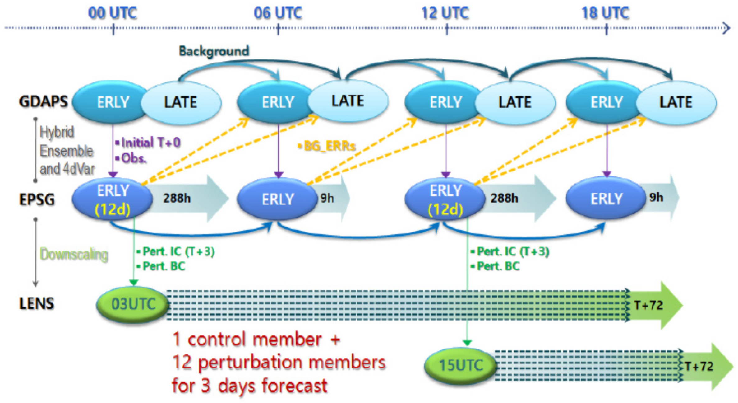
The ensemble forecasts of LLWS at intervals of 3h for lead times of 72 h (3 days) were issued twice a day at 0000 UTC (9 am local time) and 1200 UTC (9 pm local time). We focused on the LENS ensemble runs initialized at 0000 UTC. If any of the LLWS ensemble forecasts and analysis data (or both) were missing, all corresponding datasets were removed. Thereafter, the data used in the analysis were converted into seasonal data for all grid points and projection times. The verification is grid to grid.
In order to assess the reliability (or statistical consistency) of LLWS ensemble forecasts and their corresponding observations, which mean LDAPS analyses, a rank histogram [17,18] was used. The rank histogram is a very useful visual tool for evaluating the reliability of ensemble forecasts and identifying errors related to their mean and spread. Given a set of observations and a K-member ensemble forecasts, the first step in constructing a rank histogram is to rank the individual forecasts of a K-member ensemble from the lowest value to highest value. Next, a rank of the single observation within each group of K+1 values is determined. For example, if the single observation is smaller than all K-members, then its rank is 1. If it is greater than all the members, then its rank is K+1. For all sample of ensemble forecasts and observations, these ranks are plotted in the form of a histogram. If the rank histogram has a uniform pattern, then one may conclude that the ensemble and observation are drawn from indistinguishable distribution, whereas a non-uniform rank histogram indicates that the ensemble and observation are drawn from different distributions [17].
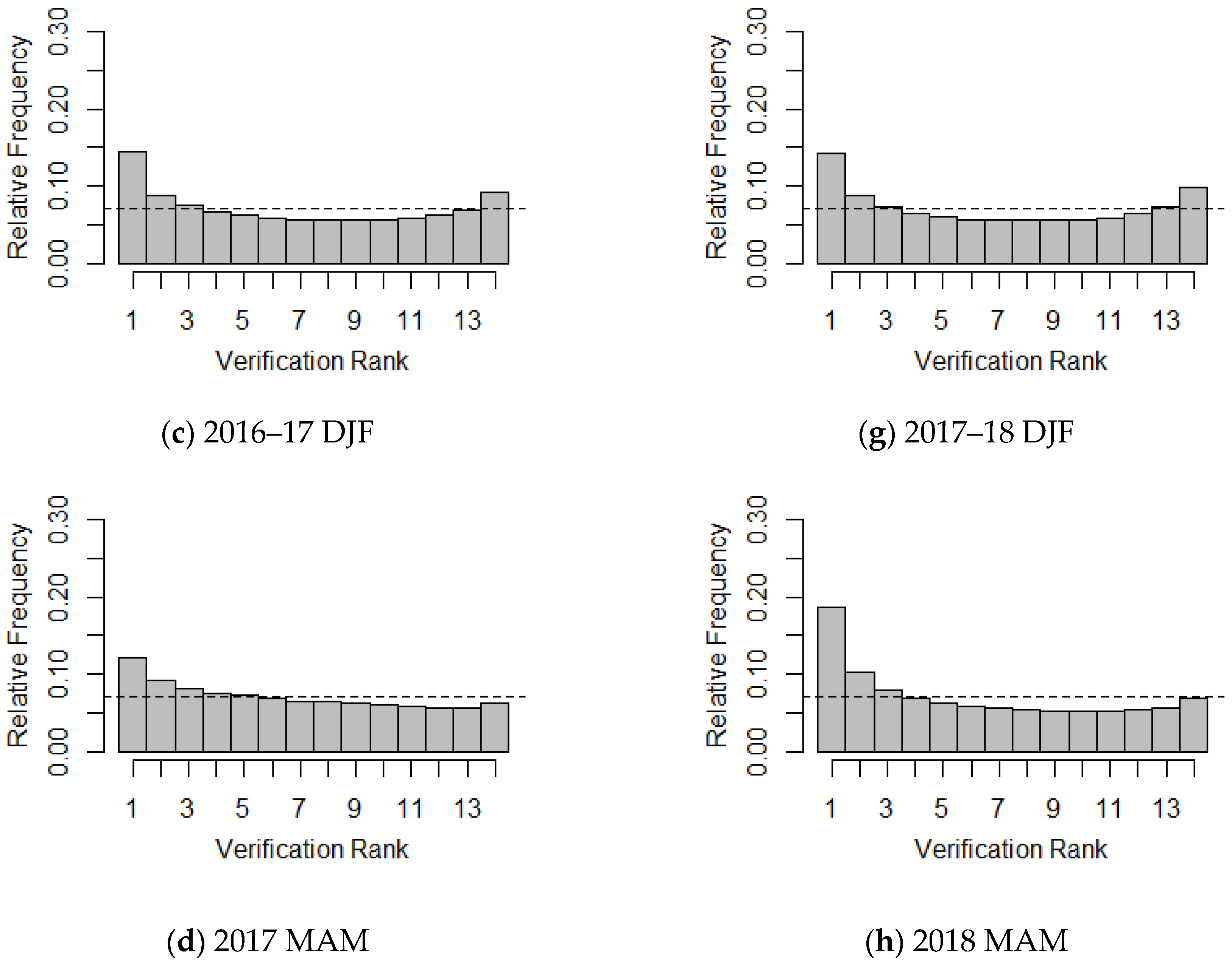
For example, a rank histogram with high (or moderate) frequency counts at both extremes, which shows a U-shaped implies the ensemble may be under-dispersive (for example Figure 4a–d,g,h). A rank histogram with high counts near one extreme and low frequency counts near the other extreme (for example, Figure 4h) presents a consistent bias or systematic error in the ensemble.
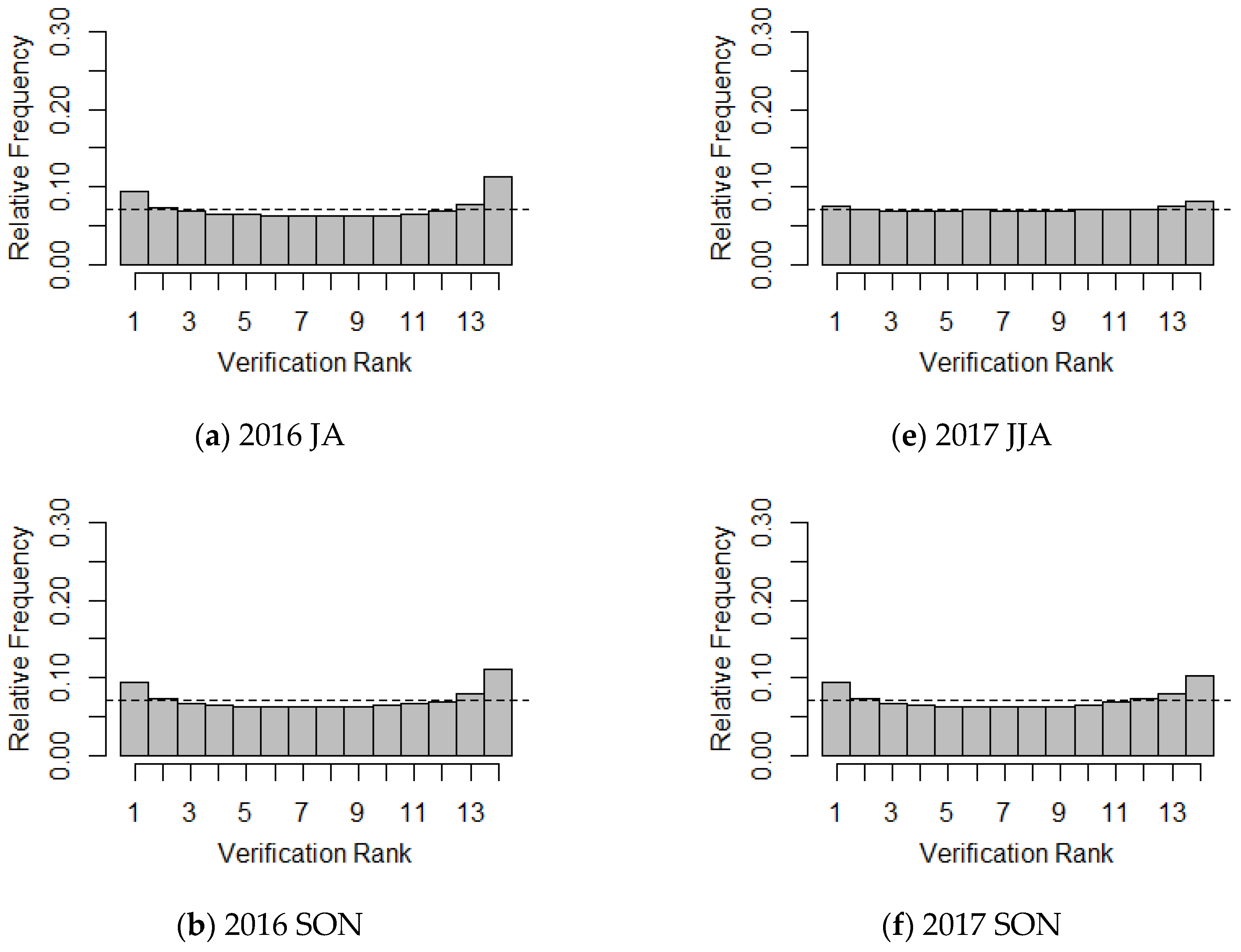
The rank histograms (RHs) for 13 ensemble forecasts and the corresponding LDAPS analyses for each season are presented in Figure 4. In general, the RHs show similar patterns according to the seasons. For JJA and SON, the RH shows that the ensemble forecast tends to have a weak trend. For the 2016 JA and SON, the RH shows nearly similar frequency counts on both extremes, but has slightly more frequency on the right. Therefore, the LLWS ensemble forecasts have a slightly negative bias, which indicates a minor under-estimation, indicating that the LLWS ensemble forecasts are generally lower than the LDAPS analyses. However, for other seasons except 2017 JJA, the LLWS ensemble forecasts have a consistently positive bias, which implies over-estimation, in particular, the RH for the 2018 MAM has a strong positive bias compared to other seasons. The RHs for the 2017 JJA and SON do not show any skewed patterns, and it can be seen that there is almost no tendency in the two seasons. Moreover, the RHs clearly show a U-shape, except in the 2017 JJA, thus verifying that ensemble forecasts have under-dispersion, which implies that the ensemble spread is smaller than that of the corresponding LDAPS analyses, although the degree to which this was true varied seasonally. In addition, we see that about 21% of the LLWS observed data are not covered by the current LLWS ensemble forecast derived from LENS. However, the RH for the 2017 JJA has an almost uniform distribution, which indicates that the LDAPS analyses and ensemble forecasts were derived from the same distribution.
The reliability index is used to quantify the deviation of the RH from uniformity [32]. The reliability index is defined by k = 1 K | p k 1 K | , where K and p k denote the number of classes in the rank histogram and the observed relative frequency in class k , respectively. If the LLWS ensemble forecasts and the corresponding LLWS observed data may have come from the same distribution, the reliability index should be zero. The reliability indexes for Figure 4 are presented in Table 1 and show a lack of uniformity (except in the 2017 JJA, as mentioned above). The reliability index of the 2018 MAM is greater than those of other seasons.
In order to examine the prediction skill of the LLWS ensemble forecasts, the ensemble mean is used. Figure 5 shows examples of the LLWS mean and spread based on grid points at a forecast time of 69-h (18 December 2016) and 60-h (8 May 2017). Line contours indicate the mean values, while the shaded colors denote the spreads. The dark blue colored regions show that the uncertain LLWS forecasts are large. The ensemble spread is the variability range for the LLWS forecasts, indicating the forecast uncertainty. The area with a large ensemble mean also has a large spread, and as the spread increases, the prediction uncertainty also increases.
The MAE, RMSE, CRPS [18,33], spread, and bias (observation-forecast) were used to assess the prediction skill of the ensemble mean. The CRPS is defined as the sum of squared differences between the cumulative distribution function, noted F , and that of the observation y , crps ( F ,   y ) = ( F ( x ) 1 ( x y ) ) 2 d x , where 1 ( · ) is the indicator function.
The prediction skill of the ensemble mean for each season is given in Figure 6. It can be seen that four measurements (except bias) have similar patterns according to the season. Also, the performance of the prediction error in the winter season is better than that of the other seasons, and the spring season consistently has the worst performance. This is because the variability between the ensemble member forecasts and LDAPS analyses increases since the frequency of severe LLWS events in the spring season is higher than in other seasons. Bias in the autumn is less than that during other seasons and the bias is largest in spring. In particular, a negative bias occurred in the autumn 2017, suggesting a positive bias.
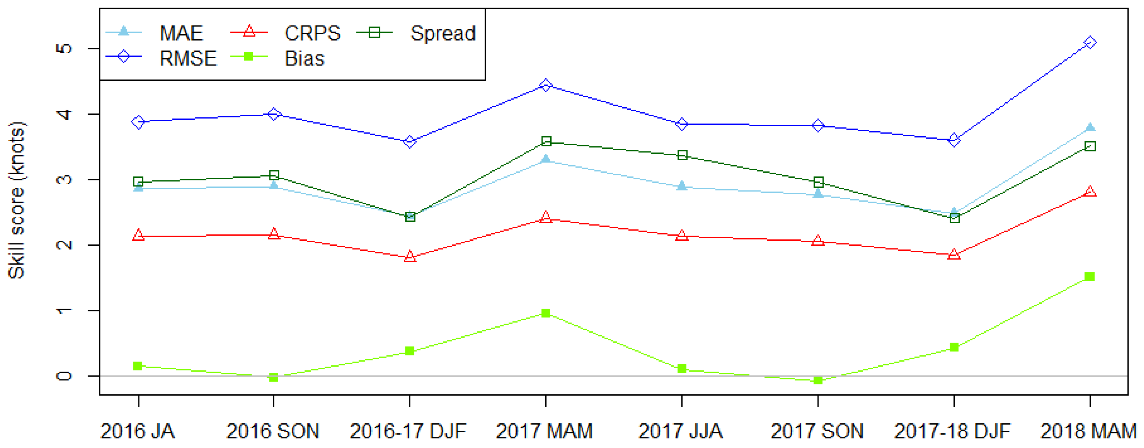
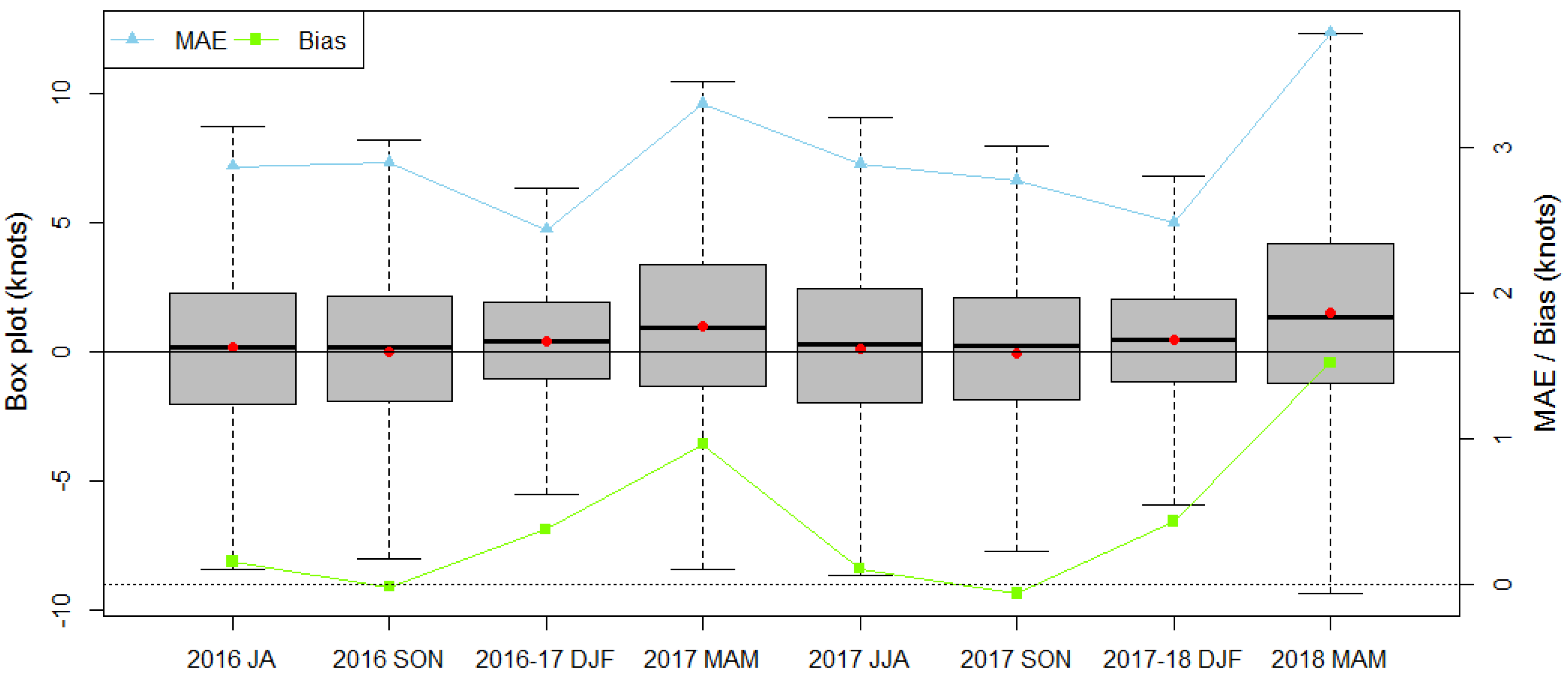
The pattern of bias according to each season is different from the results of MAE, RMSE, or CRPS, which are obtained via LLWS ensemble forecasts. Although autumn tends to have small biases, the MAE or CRPS indicate small values in winter seasons. To examine the discrepancy, box plots of the deviation between the LDAPS analyses and forecasts for each season are given in Figure 7. The average deviation (red dot) in autumn is smaller than that in winter, but the variation of the deviations in autumn is larger than that in winter. For this reason, even if the average deviation in autumn is small, the variability of the deviations is large. Therefore, the performance skill is worse in autumn than in winter. As mentioned above, spring seasons have a strong positive bias, and the corresponding variabilities have wider ranges than they do in other seasons. This demonstrates that the prediction skill in spring is not as good as in other seasons.

3.1. Reliability Analysis of Forecast Probability

The forecast probability of LLWS can be generated by using a particular threshold value. Since a severe LLWS greatly impacts aviation weather forecasts, the occurrence of a severe LLWS is defined by the following threshold:
severe   LLWS = { 1 , LLWS > 20   knots / 2000   feet 0 ,   otherwise
By using 13 ensemble member forecasts derived from LENS, the forecast probability of LLWS ensembles is computed as follows:
p ( x ) = n t n x
where n x denotes the number of ensemble members and n t denotes the number of ensemble members that are greater than 20 knots/2000 feet.
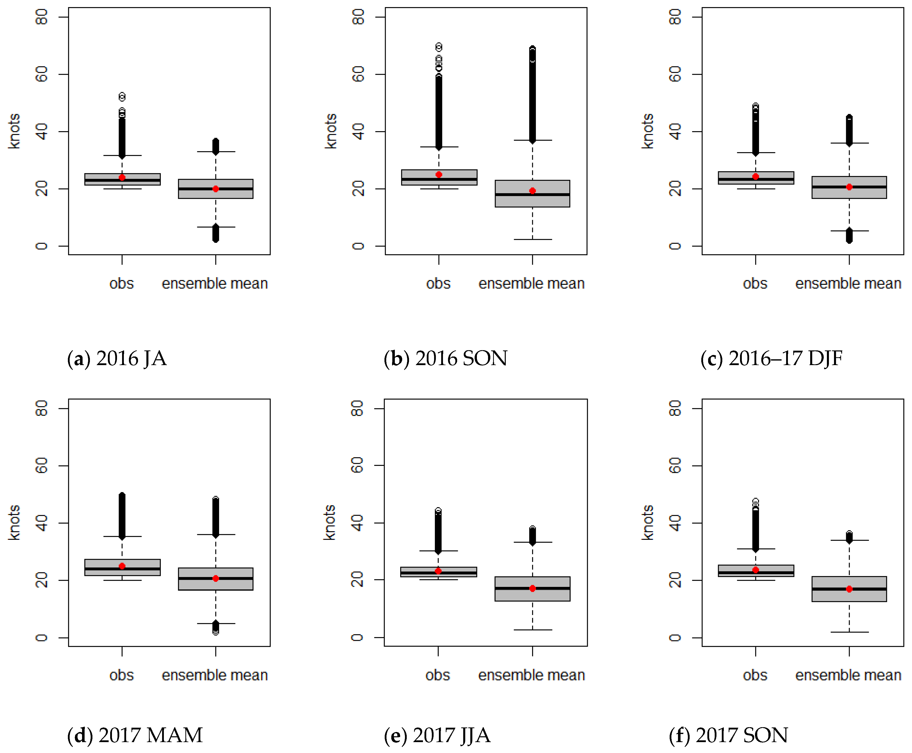
Severe LLWS events and their forecast probability, as defined in Equations (2) and (3) are calculated by using an LLWS ensemble forecast and its corresponding LDAPS analyses for each season. The distributional patterns of the LDAPS analyses and LLWS ensembles according to the presence or absence of a severe LLWS event can be analyzed by using box plots. 
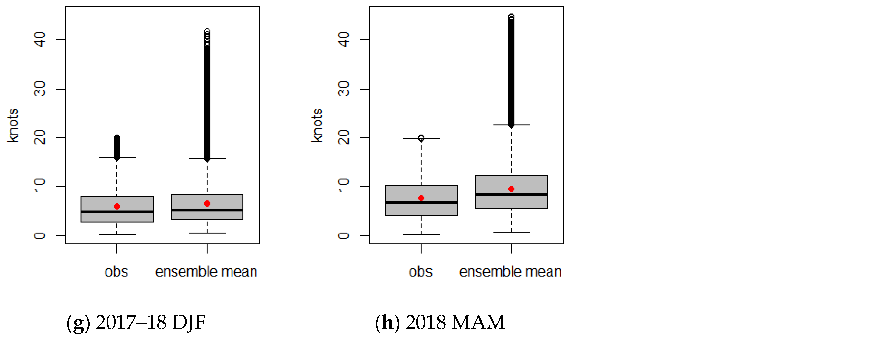
Figure 8 depicts box plots for wind speeds of the LDAPS analyses and average ensemble mean when a severe LLWS event did not occur. The distributional characteristics (mean and variation) of the observation and ensemble mean are almost similar regardless of the seasons. However, the outliers in the ensemble mean are relatively frequent compared to the LDAPS analyses. For the case of a severe LLWS in 
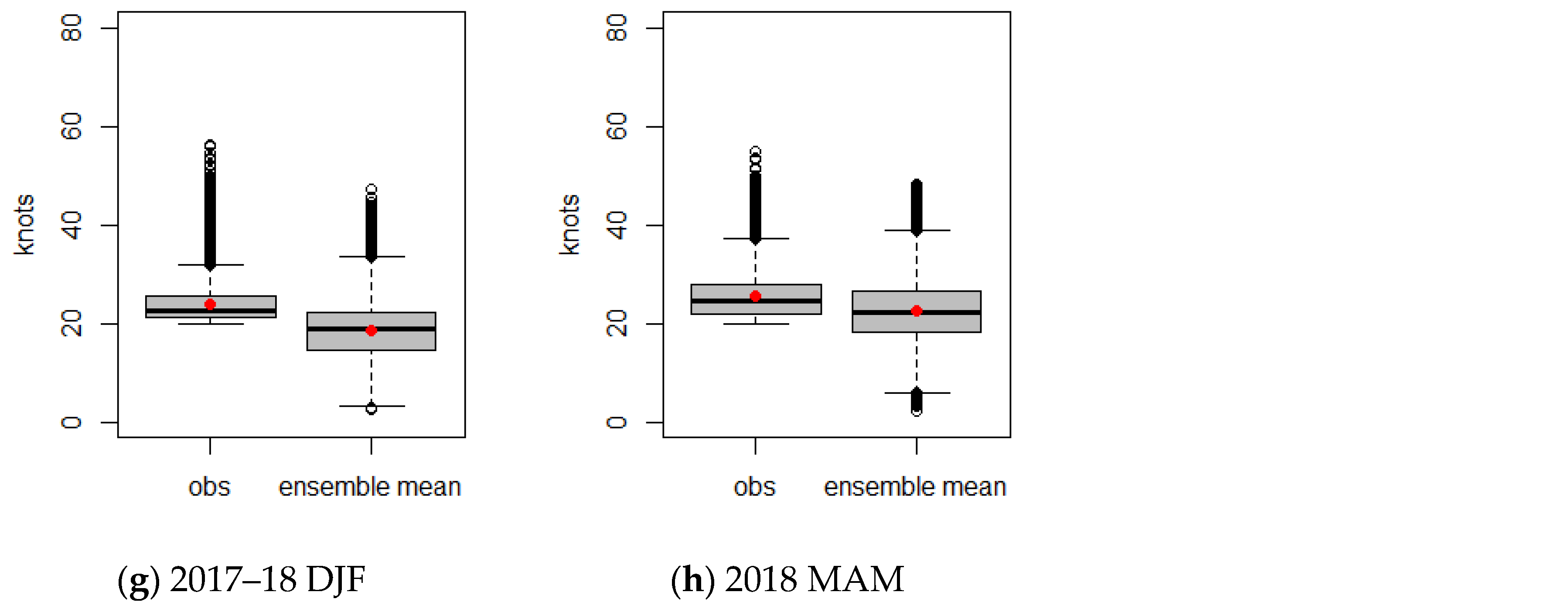
Figure 9, the wind speeds of the LDAPS analyses and average ensemble mean show different distributional patterns. The average wind speed of the LDAPS analyses is about 24 knots, which is greater than the overall ensemble mean average and has less spread than that of the ensemble mean. On the other hand, the overall ensemble mean average is smaller than the average wind speed of the LDAPS analyses and shows a large amount of variability. This suggests that the ensemble forecasts did not simulate the LDAPS analyses well when a severe LLWS occurred. It can be seen that the prediction for a future quantity of LDAPS analyses is likely to be poorly predicted.
In general, the forecast probability of LLWS events can be assessed in terms of accuracy and reliability. The Brier score can be used to assess the accuracy and the reliability of the forecast probability is evaluated by a reliability diagram.
Forecasts are classified into two categories to produce a binary forecast: the probability of a severe LLWS event (>20 knots/2000 feet) and the probability of a non-severe LLWS (otherwise). The Brier score (BS) [19,20] for a data set comprising a series of forecasts and the corresponding observations is the average of the individual scores:
BS = 1 N k = 1 N ( f k o k ) 2 ,
where N is the total number of data points, f k denotes the forecast probability of the k th ensemble member forecasts and o k is the corresponding observation with o k = 1 for the observation of a severe LLWS event and o k = 0 , otherwise. The BS is negatively oriented, with perfect forecasts exhibiting BS = 0.
The BS can be decomposed into three additive components: reliability, resolution, and uncertainty. The components of the decomposition of the BS are as follows:
BS = 1 N k = 1 K n k ( f k o k ) 2 1 N k = 1 K n k ( o ¯ k o ¯ ) 2 + o ¯ ( 1 o ¯ )
where K is the number of forecast categories, f k denotes the forecast probability of a severe LLWS event in category k , the number of observations in each category is denoted by n k , and the number of observations of a severe LLWS event in each category is denoted by o k . The average frequency of severe LLWS observations in category k is o ¯ k = o k / n k . The overall average frequency of the severe LLWS observations is o ¯ = k o k / N .
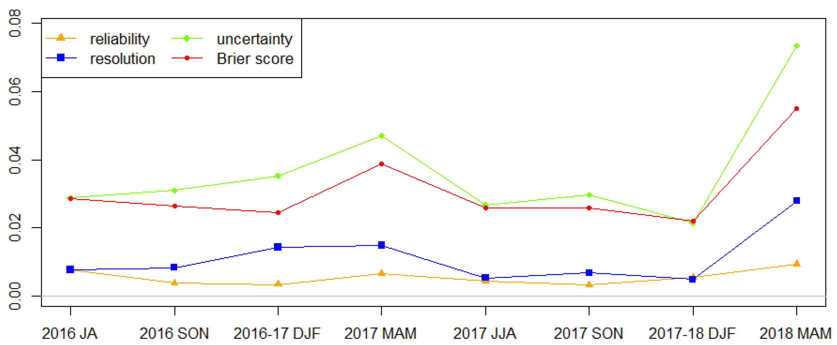
The BS, reliability, resolution, and uncertainty of the forecast probability of LLWS ensembles are described in Figure 10. For a seasonal BS, the skill of the forecast probability is the worst in the spring season. The other seasons show similar BS values, but the performance of the forecast probability in the winter season is the best. The reason the BS is poor during the spring season is that it is heavily influenced by uncertainty rather than that by other decompositions of the BS. This is because the occurrence frequency of a severe LLWS event is higher than in other seasons, thus providing a cause of increasing uncertainty.
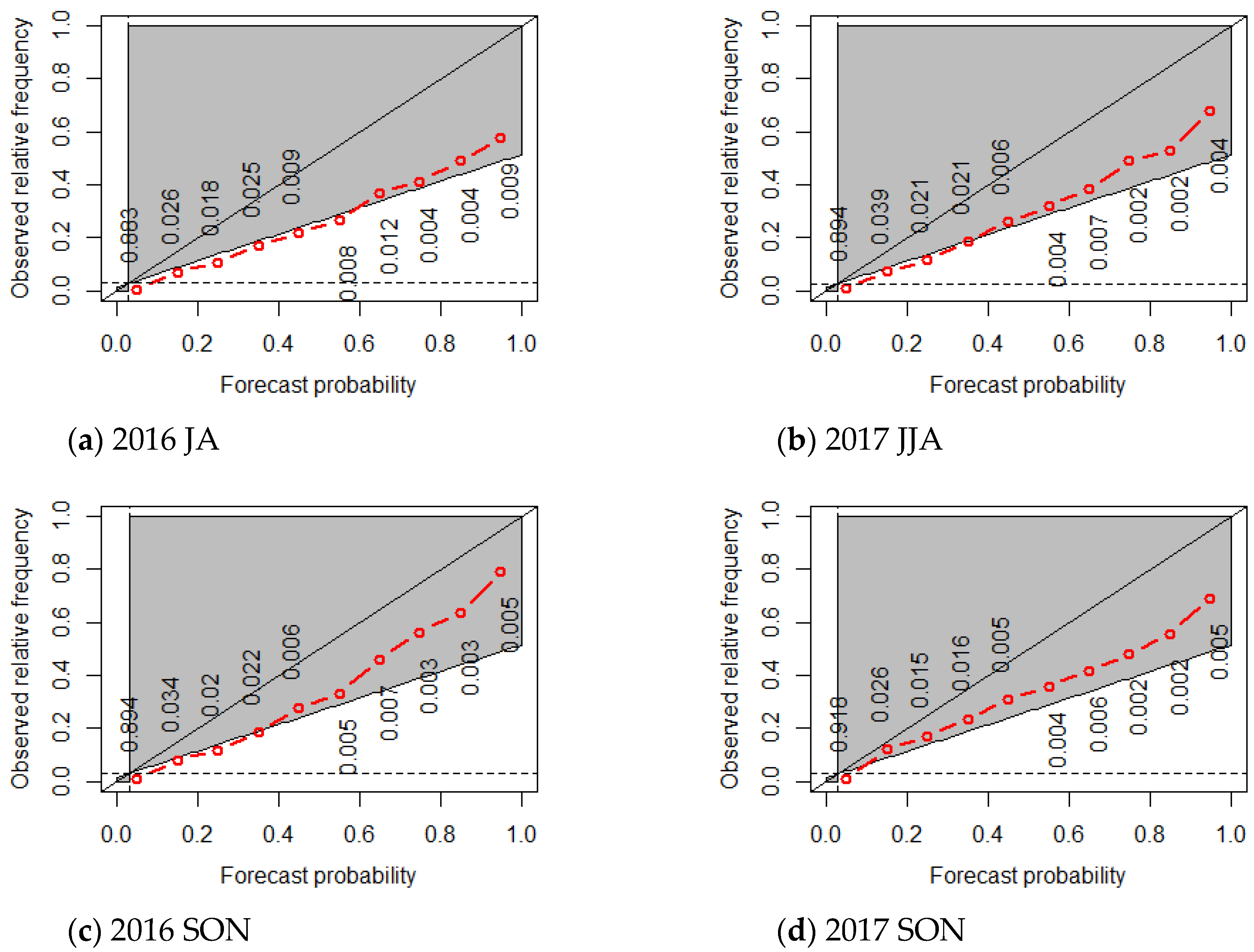
The reliability diagram is a highly useful visual tool that evaluates the reliability of the observed frequency of severe LLWS events plotted against the forecast probability of severe LLWS events [21]. The reliability diagram shows how often a forecast probability actually occurred. For perfect reliability, the forecast probability and frequency of occurrence should be equal, and the plotted points should align on the diagonal. Thus, for example, when the forecast states an event will occur with a probability of 30%, for perfect reliability, the event should occur on 30% of the occasions for which the statement was made.
To evaluate the reliability of the forecast probability of LLWS ensembles, consider the seasonal reliability diagram given in Figure 11. From Figure 11, it can be seen that the reliability curve is located below the diagonal line for all seasons, which means it is over-forecasting. Comparing the two winter seasons, since the reliability curve for the 2017–2018 DJF moves away from the best line (in contrast to the 2016–2017 DJF), the reliability of the LLWS ensembles is lower in the 2017–2018 winter. This pattern is similar in other seasons.
The resolution is obtained from the distance between the uncertainty line and the reliability curve. If the reliability curve decreases down to the uncertainty line, the LLWS ensemble forecast has no resolution, or it indicates that the forecast cannot be distinguished from data uncertainty. The gray area in Figure 11 is the skillful area, in which the LLWS ensemble forecast has skill, and the blank area is the area in which the LLWS ensemble forecast has no skill. For example, in the 2016 JA, if the LLWS ensemble forecast probability is lower than 60%, all the reliability curves are within the blank area, indicating that forecasts of severe LLWS events will not be skillful. For the 2017 MAM, when the forecast probability is equal to 0, the sample frequency is about 83.5%. This indicates that, of all the sample in 83.5% of the regions, no ensemble member indicated LLWS > 20 knots/2000 feet, indicating that all members predicted no severe LLWS event.

3.2. Forecast Probability Threshold Selection of LLWS

The occurrence of a severe LLWS can be categorized into four groups after a classification rule, as denoted in a 2 × 2 confusion matrix (contingency table) given in Table 2, which contains information about the true and predicted classes.
In Table 2, the terms positive (P) and negative (N) refer to the classifier’s prediction, and the terms true and false refer to whether that prediction corresponds to the observation. A “hit” is the number of occurrences where the forecast mean LLWS and the severe LLWS events are larger than the severe LLWS threshold. A “miss” is the number of occurrences where the forecast mean is not severe, but the observed LLWS event is severe; “false alarms” is the number of occurrence in which the forecast mean is severe, but the observed LLWS event is not severe. Several measures can be derived using the confusion matrix given in Table 2:
Hit   Rate :   HR = Hit misses + Hit
False   Alarm   Rate :   FAR = False   Alarms Hit + False   Alarms ,
Missing   Rate   =   1 - HR ,
Equitable   Threat   Score :   ETS = Hit Hit random Hit + misses + False   Alarms Hit random ,
where
Hit random = ( Hit + misses ) ( Hit + False   Alarms ) N .
First, we consider the forecast probability distribution obtained from 13 ensemble member forecasts to select the forecast probability threshold. 
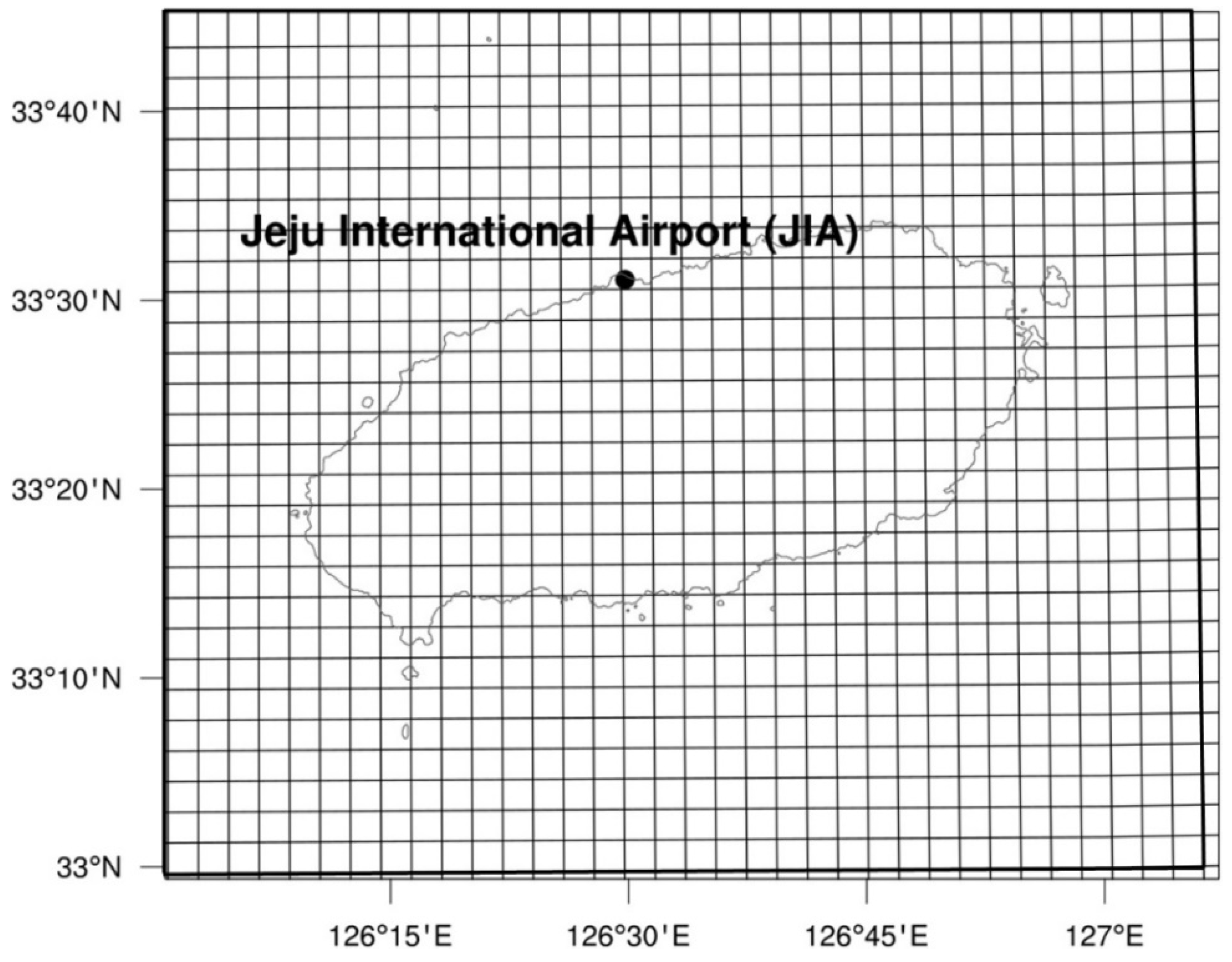
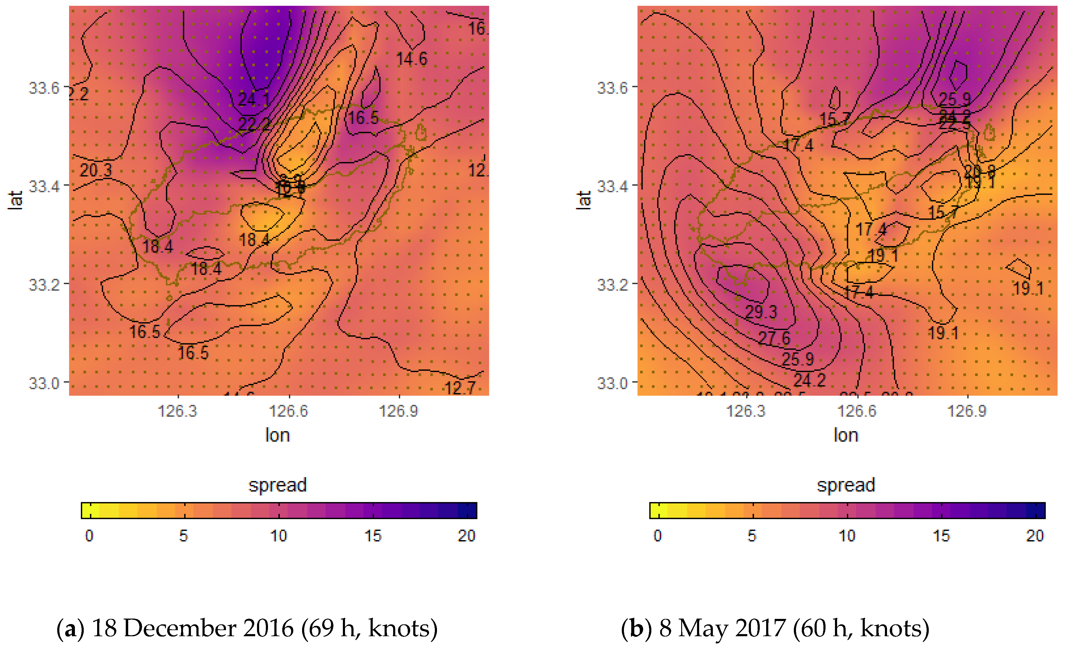
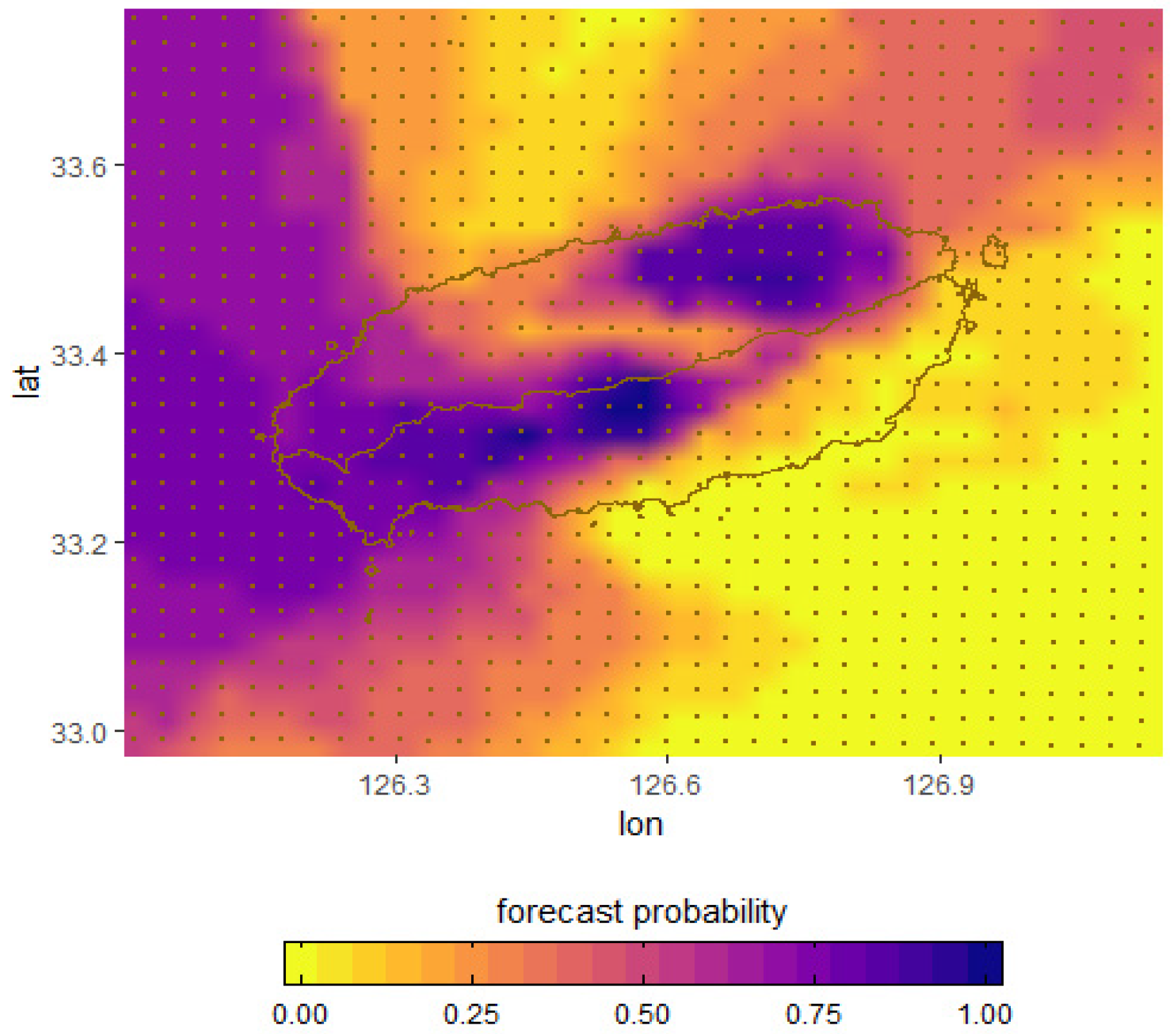
Figure 12 shows the severe LLWS probability distributions for all grid points of the Jeju area at the projection time of 24 h on 9 May 2017.
In Figure 12, the yellow areas indicate that the forecast probability of a severe LLWS event is zero, and the blue areas indicate the most likely regions in which an LLWS event is over 20 knots/2000 feet. Depending on the region, the inland areas with dark blue are areas in which a severe LLWS event is more likely to occur, while other regions have different forecast probabilities for the severe LLWS. In this case, it is necessary to choose an appropriate threshold for the forecast probability to issue a severe LLWS warning for some regions. If the threshold sets to higher, the forecast confidence will increase but it will also lead to a high missing rate. On the other hand, if it is set to lower, the missing rate may be decreased, while the FAR increases. Therefore, determining a forecast probability threshold to issue severe LLWS warnings for certain regions is an important issue. For example, if the threshold is set to 100%, then all ensemble members will provide a severe LLWS forecast, and the confidence will be highest. Some regions in which a severe LLWS event actually happens, however, might be missed, but not all members will provide a severe LLWS forecast. If the threshold is set to 50%, then the missing rate may be lowered, but it may increase the FAR and the confidence level may decrease since only 50% of the members predict a severe LLWS event. Therefore, the issues with regard to the probability threshold is a very practical problem for forecasters interested in utilizing the probability information.
According to the methods of Zhou et al. [16], we therefore select a forecast probability threshold using the ETS. Both the missing rate and FAR are related to the ETS and if both are at their lowest then the ETS will be at its highest. To select a threshold, we computed the missing rate and the FAR as well as the ETS for different forecast probabilities and selected a threshold in which both the missing rate and the FAR are their lowest and the ETS at their highest.
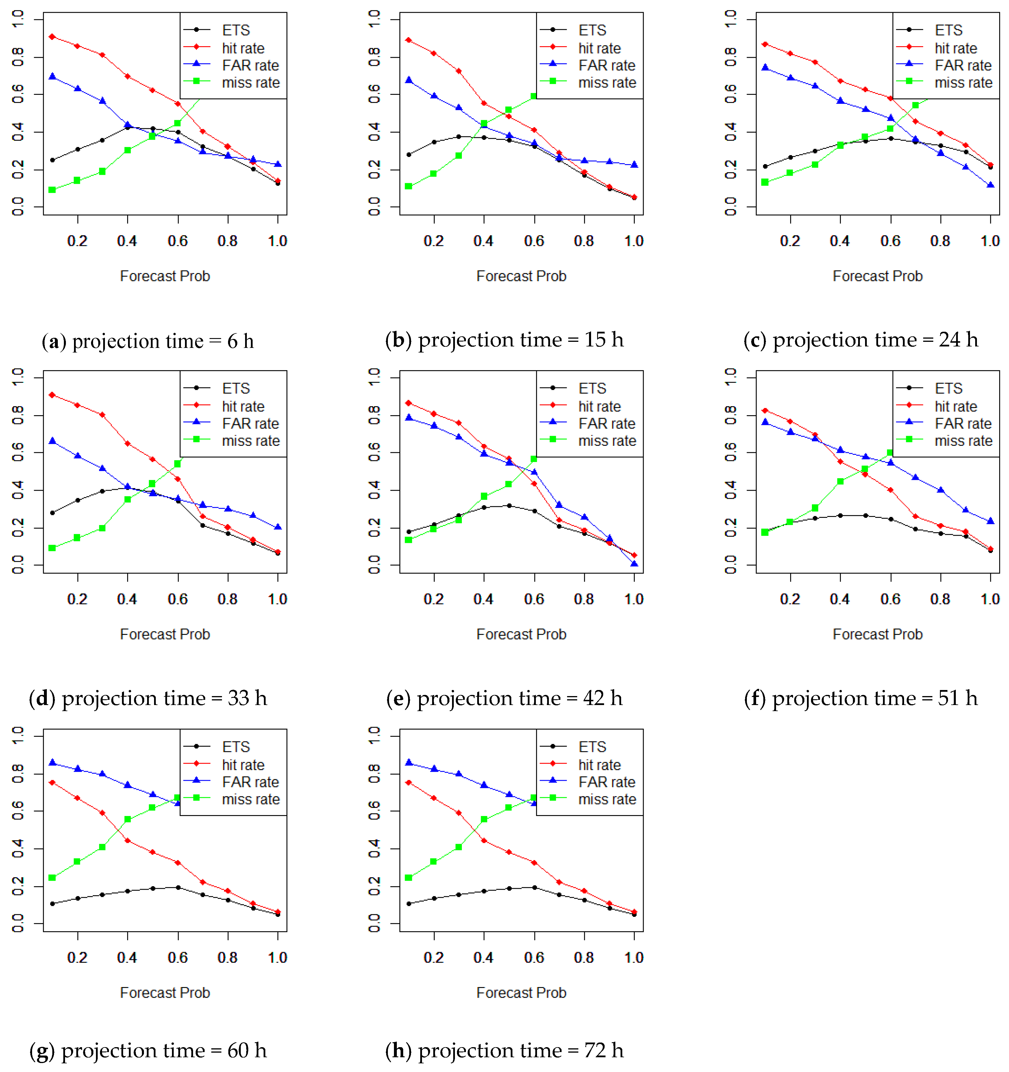
For each season, the missing rate, hit rate, FAR and ETS were calculated for different forecast probabilities to select a threshold of the forecast probability for each season on 34 × 28 grid points of Jeju at each projection time and depicted them together in one plot. For each season, we set the threshold of the forecast probability at intervals of 3 h for lead times up to 72 h. Figure 13 describes how to select a forecast probability threshold for issuing a severe LLWS. In Figure 13, the red, blue, green and black lines denote the hit rate, FAR, missing rate, and ETS, respectively. From Figure 13, it can be seen that the optimal forecast probability threshold is different depending on the projection times. For the projection time of 6 h, the results show that the best probability threshold is about 50%, where the ETS has a maximum point when the sum of the missing rate and the FAR is lowest. This means that the forecast probability threshold should be selected at 50% for issuing a severe LLWS warning. That is, as long as an area has a severe LLWS probability > 50%, we can be relatively confident that a severe LLWS will happen; this approach makes it most likely to miss a severe LLWS but has the lowest FAR.
For other projection times, we should select 40% at a projection time of 15 h, 60% at a projection time of 24 h, 45% at a projection time of 33 h, 55% at a projection time of 42 h, 55% at a projection time of 51 h, 60% at a projection time of 60 h and 60% at a projection time of 72 h. For other seasons, different forecast probability thresholds are obtained depending on the projection times (e.g., the 2017 MAM, Figure 13).
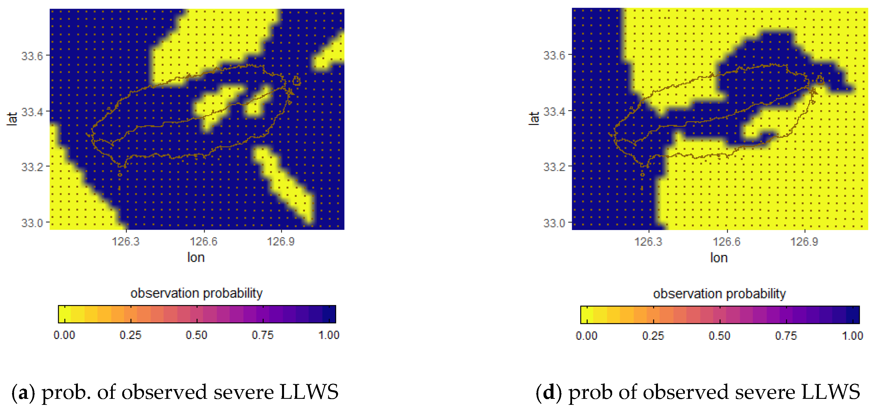
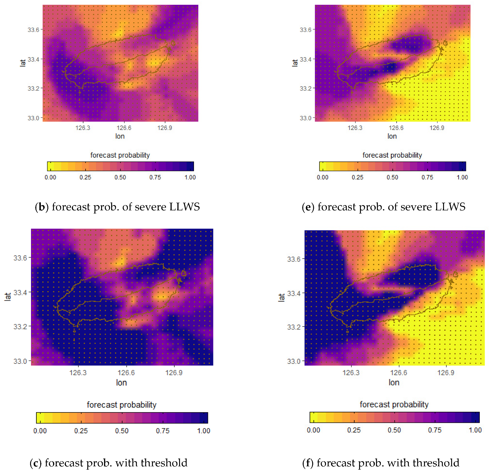
The observed probability, the forecast probability obtained from raw ensembles, and the best probability threshold for issuing a severe LLWS forecast for projection times of 60 h and 24 h on May 8 and 9, 2017 are respectively given in Figure 14. From Figure 14a, the probability of the observed severe LLWS has a binary value. That is, if the observed LLWS is greater than 20 knots/2000 feet, then the probability of a severe LLWS event is equal to 1 (blue region); otherwise, it is 0 (yellow region). Figure 14b also represents the forecast probability of the LLWS ensembles defined in Equation (4). Comparing the observed probability (Figure 14a) with the forecast probability (Figure 14b) for the severe LLWS, the forecast probabilities are not consistent with the observed probabilities in most regions; that is, the forecast probabilities are predicted to be smaller than the observed probabilities. The forecast probability of a severe LLWS event is given in Figure 14c when the best probability threshold is applied. In Figure 14c, we selected 60% as the forecast probability threshold for issuing a severe LLWS warning. The forecast probability with threshold (Figure 14c) is obtained as the forecast probability of severe LLWS (Figure 14b) is divided by the threshold of 0.6 for all grid points. The ratio can be less than or greater than 1. If it is greater than 1, it is set to 1. The forecast probability distribution that is applied to the best probability threshold is similar to the observed probability distribution. It can be seen that regions where the forecast probability of a severe LLWS event is more than 60% are much more similar to regions where actual severe LLWS events occur compared to regions in which the threshold is not applied. Figure 14d–f gives the probability distribution of the observed severe LLWS, the forecast probability obtained from LLWS ensembles, and the forecast probability from applying the threshold; the forecast probability threshold was set to 60%. It can be seen that the forecast probabilities obtained from LLWS ensembles are predicted to be lower than the probabilities of the observed severe LLWS events, except in some regions. This indicates that there is not a high possibility of issuing a severe LLWS warning. However, when the threshold is applied, the probability distribution of the regions where the forecast probability is greater than 60% are much more similar to those of regions in which the observed severe LLWS occurred. Therefore, we can see that the selection of a threshold plays an important role in issuing a severe LLWS warning.
We used only the hit rate, missing rate, FAR, and ETS to determine the best threshold. However, there is a limit to setting an optimal threshold using the hit rate, missing rate and FAR. If the frequency of occurrence of the observed severe LLWS events is not high, then a severe LLWS rarely occurs. In that case, any one of these rates can have a value of zero, and we cannot select a probability for which, both the missing rate and the FAR are lowest. To solve this problem, a lot of data should be provided, or as mentioned by Zhou et al. [16], the economic factors that have an impact on the probability threshold selection rule should be considered.

4. Conclusions

LLWS is one of the major concerns of aviation weather forecasters at airports because of its dangerous impact on airplane landing operations and management. However, there have been few studies on ensemble verification and forecasts of LLWS. Therefore, we conducted a reliability analysis and evaluation to verify LLWS ensemble member forecasts and LDAPS analyses based on grid points over the Jeju area.
A rank histogram, BS, and a reliability diagram were used to identify the statistical consistency of LLWS ensemble forecasts and their corresponding LDAPS analyses. It was found that LLWS ensemble forecasts have negative (summer and autumn seasons) or positive biases (spring and winter seasons). The reliability curve also indicated that the ensemble forecast was over-forecasting LLWS events.
The selection of a forecast probability threshold from the LLWS ensemble forecast is one of the most important factors for issuing a severe LLWS warning. We utilized a simple method to select a forecast probability threshold without considering economic factors. We selected seasonal forecast probability thresholds to issue the appropriate severe LLWS warning for each forecast time. The results indicate that a reasonable probability threshold is important for issuing a severe LLWS warning. The selection, however, is dependent on data characteristics, the size of the datasets, the frequency of severe LLWS events, etc. Therefore, there is a limit to setting an optimal probability threshold using hit rates, missing rates, FAR, and ETS. If a severe LLWS occurs rarely and the dataset is small, then the hit rate or other measures can be zero. In cases like these, we cannot determine a threshold in which both the missing rate and the FAR are at their lowest and the ETS is at its highest.
This work can be considered an early approach to applying bias-correction techniques. The systematic and random errors based on the primary results may be reduced by using statistical post-processing methods for LLWS. If the bias-corrected LLWS can be used in prediction, the skill will be better than that of the current LLWS forecast.

Author Contributions

Conceptualization, H.W.C., Y.-G.L. and S.-B.R.; methodology, C.K.; software, C.K. and K.H.; validation, Y.-G.L. and C.K.; formal analysis, C.K. and K.H. All authors have read and agreed to the published version of the manuscript.

Funding

This work was funded by the Korea Meteorological Administration Research and Development Program “Research and Development for KMA Weather, Climate, and Earth system Services–Support to Development of Techniques for Bio- and Industrial-Meteorology” under Grant KMA2018-00621.

Conflicts of Interest

The authors declare no conflict of interest.

References

  1. Weather-Related Aviation Accident Study 2003–2007. In Federal Aviation Administration (FAA) Aviation Safety Information Analysis and Sharing (ASIAS); Federal Aviation Administration (FAA): Washington, DC, USA, 2010.
  2. Ministry of Land, Infrastructure, and Transport (MOLIT). Aviation Market Trend & Analysis. Aviat. Policy Div. 2018, 55, 120–121. (In Korean) [Google Scholar]
  3. Merritt, M.W.; Klingle-Wilson, D.; Campbell, S.D. Wind Shear Detection with Pencil-Beam Radars. Linc. Lab. J. 1989, 2, 483. [Google Scholar]
  4. Wilson, F.W.; Gramzow, R.H. The redesigned Low Levels Wind Shear Alert System. In Proceedings of the 4th International Coference on Aviation Weather Syst, Paris, France, 24–28 June 1991; p. 370. [Google Scholar]
  5. Boilley, A.; Mahfouf1, J.-F. Wind shear over the Nice Côte d’Azur airport: Case studies. Nat. Hazards Earth Syst. Sci. 2013, 13, 2223–2238. [Google Scholar] [CrossRef] [Green Version]
  6. Chan, P.W.; Hon, K.K. Performance of super high resolution numerical weather prediction model in forecasting terrain-disrupted airflow at the Hong Kong International Airport: Case studies. Meteorol. Appl. 2016, 23, 101–114. [Google Scholar] [CrossRef]
  7. Zhu, Y. Ensemble Forecast: A New Approach to Uncertainty and Predictability. Advs. Atmos. Sci. 2005, 22, 781–788. [Google Scholar] [CrossRef]
  8. Bowler, N.E.; Arribas, A.; Beare, S.E.; Mylne, K.R.; Shutts, G.J. The local ETKF and SKEB: Upgrade to the MOGREPS short-range ensemble prediction system. Quart. J. Roy. Meteorol. Soc. 2009, 135, 767–776. [Google Scholar] [CrossRef]
  9. Du, J.; Deng, G. The utility of the transition from deterministic to probabilistic weather forecasts: Verification and application of probabilistic forecasts. Meteorol. Mon. 2010, 36, 10–18. [Google Scholar]
  10. Kühnlein, C.; Keil, C.; Craig, G.C.; Gebhardt, C. The impact of downscaled initial condition perturbations on convective-scale ensemble forecasts of precipitation. Quart. J. R. Meteor. Soc. 2014, 140, 1552–1562. [Google Scholar] [CrossRef]
  11. Dey, S.R.; Leoncini, A.G.; Roberts, N.M.; Plant, R.S.; Migliorini, S.A. spatial view of ensemble spread in convection permitting ensembles. Mon. Wea. Rev. 2014, 142, 4091–4107. [Google Scholar] [CrossRef] [Green Version]
  12. Dey, S.R.; Roberts, N.M.; Plant, R.S.; Migliorini, S.A. new method for characterization and verification of local spatial predictability for convective-scale ensembles. Quart. J. Roy. Meteor. Soc. 2016, 142, 1982–1996. [Google Scholar] [CrossRef] [Green Version]
  13. Szczes, J. Communicating Optimized Decision Input from Stochastic Turbulence Forecasts. Master’s thesis, Naval Postgraduate School, Monterey, CA, USA, March 2008. [Google Scholar]
  14. Gill, P.G.; Buchanan, P. An ensemble based turbulence forecasting system. Meteorol. Appl. 2014, 21, 12–19. [Google Scholar] [CrossRef]
  15. Zhou, B.; Du, J.; McQueen, J.; Dimego, G.; Manikin, G.; Ferrier, B.; Toth, Z.; Jung, H.; Han, J. An introduction to NCEP SREF Aviation Project. In Proceedings of the 11th Conference on Aviation Range and Aerospace, Hyannis, MA, USA, 4–8 October 2004. [Google Scholar]
  16. Zhou, B.; McQueen, J.; Du, J.; DiMego, G.; Toth, Z.; Zhu, Y. Ensemble forecast and verification of low level wind shear by the NCEP SREF system. In Proceedings of the 21st Conference on Weather Analysis and Forecasting, Washington, DC, USA, 28 July–5 August 2005. [Google Scholar]
  17. Hamil, T.M. Interpretation of rank histograms for verifying ensemble forecasts. Mon. Wea. Rev. 2001, 129, 550–560. [Google Scholar] [CrossRef]
  18. Wilks, D.S. Statistical Methods in the Atmospheric Sciences, 3rd ed.; Elsevier, Academic Press: Cambridge, MA, USA, 2011; pp. 351–375. [Google Scholar]
  19. Brier, G.W. Verification of forecasts expressed in terms of probability. Mon. Wea. Rev. 1950, 78, 1–3. [Google Scholar] [CrossRef]
  20. Murphy, A.H. A new vector partition of the probability score. J. Appl. Meteorol. 1973, 12, 595–600. [Google Scholar] [CrossRef] [Green Version]
  21. Hartmann, H.C.; Pagano, T.C.; Sorooshiam, S.; Bales, R. Confidence builder: Evaluating seasonal climate forecasts from user perspectives. Bull. Amer. Meteor. Soc. 2002, 83, 683–698. [Google Scholar] [CrossRef] [Green Version]
  22. Hagelin, S.; Son, J.; Swinbank, R.; McCabe, A.; Robertsa, N.; Tennanta, W. The Met Office convective-scale ensemble, MOGREPS-UK. Q. J. R. Meteorol. Soc. 2017, 143, 2846–2861. [Google Scholar] [CrossRef]
  23. Bowler, N.; Arribas, A.; Mylne, K.; Robertson, K.; Beare, S. The MOGREPS short-range ensemble prediction system. Q. J. R. Meteorol. Soc. 2008, 134, 703–722. [Google Scholar] [CrossRef]
  24. Clayton, A.; Lorenc, A.; Barker, D. Operational implementation of a hybrid ensemble/4D-Var global data assimilation system at the Met Office. Q. J. R. Meteorol. Soc. 2013, 139, 1445–1461. [Google Scholar] [CrossRef]
  25. Lee, S.-W.; Park, J.-H.; Kim, D.-J. Limited Area Ensemble Prediction System (LENS) in KMA toward Early Warning System for High Impact Weather. In Proceedings of the Autumn Meeting of KMS, Jeju, Korea, 12–14 October 2015; pp. 237–238. [Google Scholar]
  26. Kim, S.H.; Kim, H.M.; Kay, J.K.; Lee, S.-W. Development and Evaluation of the High Resolution Limited Area Ensemble Prediction System in the Korea Meteorological Administration. Atmos. Korean Meteor. Soc. 2015, 25, 67–83. [Google Scholar]
  27. Aviation Weather Services (AWS). Terminal Aerodrome Forecasts, Operations and Services. NWS Instruction 10-813 2004, 10–18. [Google Scholar]
  28. Advanced Research on Aviation Meteorology. NIMS Annual Report of the Research and Development for KMA Applied Meteorology Services; National Institute of Meteorological Sciences (NIMS): Jeju-do, Korea, 2018; p. 76. (In Korean) [Google Scholar]
  29. Verification of KMA Numerical Prediction Systems 2018; Technical Report of KMA Numerical Modeling Center; Korea Meteorological Administration (KMA): Seoul, Korea, 2019; p. 232. (In Korean)
  30. Joint WMO technical progress report on the global data processing and forecasting system and numerical weather prediction research activities for 2016. In WMO Global Data-Processing and Forecasting System; Korea Meteorological Administration (KMA): Seoul, Korea, 2016; p. 21.
  31. Ahn, Y.; Jang, J.; Kim, K.-Y. Analysis of low level cloud prediction in the KMA Local Data Assimilation and Prediction System (LDAPS). J. Korean Soc. Avi. Aeonau 2017, 25, 124–129, (In Korean with English abstract). [Google Scholar]
  32. Delle, L.M.; Hacker, J.P.; Zhou, Y.; Deng, X.; Stull, R.B. Probabilistic aspects of meteorological and ozone regional ensemble forecasts. J. Geophy. Res 2006, 111, D23407. [Google Scholar] [CrossRef] [Green Version]
  33. Gneiting, T.; Raftery, A.E. Strictly proper scoring rules, prediction, and estimation. J. Am. Stat. Assoc. 2007, 102, 359–378. [Google Scholar] [CrossRef]
Figure 1. The schematic flow chart of the Limited area ENsemble prediction System (LENS) operated in conjunction with the Global Data Assimilation and Prediction System (GDAPS) and Ensemble Prediction System for Global (EPSG) at the Korea Meteorological Administration (KMA) (Sourced from [25]).
Atmosphere 11 00198 g001
Figure 2. (a) Horizontal domain boundaries of LENS (solid lines) and LDAPS (dashed lines) and (b) the verification (shaded) area determined from the overlapping regions of both model forecasts around the Korean peninsula.
Atmosphere 11 00198 g002
Figure 3. The orography of the 102 km × 84 km region around the Jeju International Airport (JIA). The thick rectangular area indicates the verification area of 34 × 28 grids with 3-km resolution.
Atmosphere 11 00198 g003
Figure 4. Verification rank histograms of LLWS events for each season. (a) 2016 JA; (b) 2016 SON; (c) 2016-17 DJF; (d) 2017 MAM; (e) 2017 JJA; (f) 2017 SON; (g) 2017-18 DJF; (h) 2018 MAM.
Atmosphere 11 00198 g004aAtmosphere 11 00198 g004b
Figure 5. LLWS mean (black lines) and spread (filled colors) distribution over Jeju Island (yellow green line) at (a) 69 h (18 December 2016) and (b) 60 h (8 May 2017).
Atmosphere 11 00198 g005
Figure 6. Prediction skills of the LLWS ensemble mean for each season.
Atmosphere 11 00198 g006
Figure 7. Box plot for the deviation between the LDAPS analyses and ensemble mean and the average mean absolute error (MAE) and biases for each season.
Atmosphere 11 00198 g007
Figure 8. Box plots for LDAPS analyses and the average ensemble forecasts when a severe LLWS event did not occur. The red dot and horizontal line for each box denote the mean and median of the data, respectively. (a) 2016 JA; (b) 2016 SON; (c) 2016-17 DJF; (d) 2017 MAM; (e) 2017 JJA; (f) 2017 SON; (g) 2017-18 DJF; (h) 2018 MAM.
Atmosphere 11 00198 g008aAtmosphere 11 00198 g008b
Figure 9. Box plots for LDAPS analyses and the average ensemble forecasts when a severe LLWS event was observed. (a) 2016 JA; (b) 2016 SON; (c) 2016-17 DJF; (d) 2017 MAM; (e) 2017 JJA; (f) 2017 SON; (g) 2017-18 DJF; (h) 2018 MAM.
Atmosphere 11 00198 g009aAtmosphere 11 00198 g009b
Figure 10. Reliability, resolution, uncertainty and Brier score of the LLWS for each season.
Atmosphere 11 00198 g010
Figure 11. Reliability diagram of LLWS for each season. The numbers on the panel are the sample frequency for each bin, which are obtained as the number of forecast probabilities included in the bins are divided by the total number of forecast probabilities. (a) 2016 JA; (b) 2017 JJA; (c) 2016 SON; (d) 2017 SON; (e) 2016-17 DJF; (f) 2017-18 DJF; (g) 2017 MAM; (h) 2018 MAM.
Atmosphere 11 00198 g011aAtmosphere 11 00198 g011b
Figure 12. Forecast probability distribution at 24 h, 9 May 2017.
Atmosphere 11 00198 g012
Figure 13. The best probability threshold for issuing a severe LLWS warning (2017 MAM). (a) projection time = 6 h; (b)projection time = 15 h; (c) projection time = 24 h; (d) projection time = 33 h; (e) projection time = 42 h; (f) projection time = 51 h; (g) projection time = 60; (h) projection time = 72 h.
Atmosphere 11 00198 g013
Figure 14. Forecast probability distribution of LDAPS analyses and forecasts using probability threshold. (ac) May 8, 2017 projection time 60 h; (df) May 9, 2017 projection time 24 h.
Atmosphere 11 00198 g014aAtmosphere 11 00198 g014b
Table 1. The reliability indexes for Figure 4.
SeasonReliability Index
2016 JA0.144
2016 SON0.142
2016–17 DJF0.223
2017 MAM0.173
2017 JJA0.034
2017 SON0.131
2017–18 DJF0.233
2018 MAM0.308
Note: JA = July, August; SON = September, October, November; DJF = December, January, February; MAM = March, April, May; JJA = June, July, August.
Table 2. Confusion matrix.
True Condition
Positive (P)Negative (N)
Predicted conditionPositiveHit
(TP, True, Positive)
False Alarms
(FP, False Positive)
Negativemisses
(FN, False Negative)
Correct Negative
(TN, True Negative)

