Article

Operational Modelling of Umbrella Cloud Growth in a Lagrangian Volcanic Ash Transport and Dispersion Model

by
Helen N. Webster
1,2,*,
Benjamin J. Devenish
1,
Larry G. Mastin
3,
David J. Thomson
1 and
Alexa R. Van Eaton
3
1
Met Office, FitzRoy Road, Exeter EX1 3PB, UK
2
College of Engineering, Mathematics and Physical Sciences, University of Exeter, Exeter EX4 4QF, UK
3
U.S. Geological Survey, Cascades Volcano Observatory, Vancouver, WA 98683, USA
*
Author to whom correspondence should be addressed.
Submission received: 22 November 2019 / Revised: 9 January 2020 / Accepted: 20 January 2020 / Published: 13 February 2020
(This article belongs to the Special Issue Forecasting the Transport of Volcanic Ash in the Atmosphere)

Abstract

:
Large explosive eruptions can result in the formation of an umbrella cloud which rapidly expands, spreading ash out radially from the volcano. The lateral spread by the intrusive gravity current dominates the transport of the ash cloud. Hence, to accurately forecast the transport of ash from large eruptions, lateral spread of umbrella clouds needs to be represented within volcanic ash transport and dispersion models. Here, we describe an umbrella cloud parameterisation which has been implemented into an operational Lagrangian model and consider how it may be used during an eruption when information concerning the eruption is limited and model runtime is key. We examine different relations for the volume flow rate into the umbrella, and the rate of spreading within the cloud. The scheme is validated against historic eruptions of differing scales (Pinatubo 1991, Kelud 2014, Calbuco 2015 and Eyjafjallajökull 2010) by comparing model predictions with satellite observations. Reasonable predictions of umbrella cloud spread are achieved using an estimated volume flow rate from the empirical equation by Bursik et al. and the observed eruption height. We show how model predictions can be refined during an ongoing eruption as further information and observations become available.

1. Introduction

The role of the Volcanic Ash Advisory Centres (VAACs) is to issue advisories on the location and forecasted movement of volcanic ash within the atmosphere, in order to minimise risks to the aviation community. The volcanic ash advisories are produced using a combination of volcano data, observations (from satellite, ground and aircraft), data from numerical weather prediction (NWP) models and dispersion modelling. The role is operational; hence, advisories need to be timely and frequent.
During large explosive volcanic eruptions, the buoyant ash plume can expand laterally to form an umbrella cloud [1]. Gravitational spreading can dominate the transport and dispersion of the ash cloud over distances ranging from tens to hundreds of kilometres from the source (and, for supereruptions, potentially thousands of kilometres) [2,3,4,5]. Currently, lateral spread of umbrella clouds is not typically included within the operational modelling activities conducted by VAACs using volcanic ash transport and dispersion models (VATDMs).
VATDMs typically represent advection by the mean ambient wind, diffusion due to atmospheric turbulence, and gravitational settling of ash particles; however, these models often lack parameterisations of spreading within umbrella clouds. This omission limits their ability to accurately forecast ash clouds from large explosive eruptions. In particular, the radial expansion, including upwind transport, of the ash cloud can be grossly underpredicted.
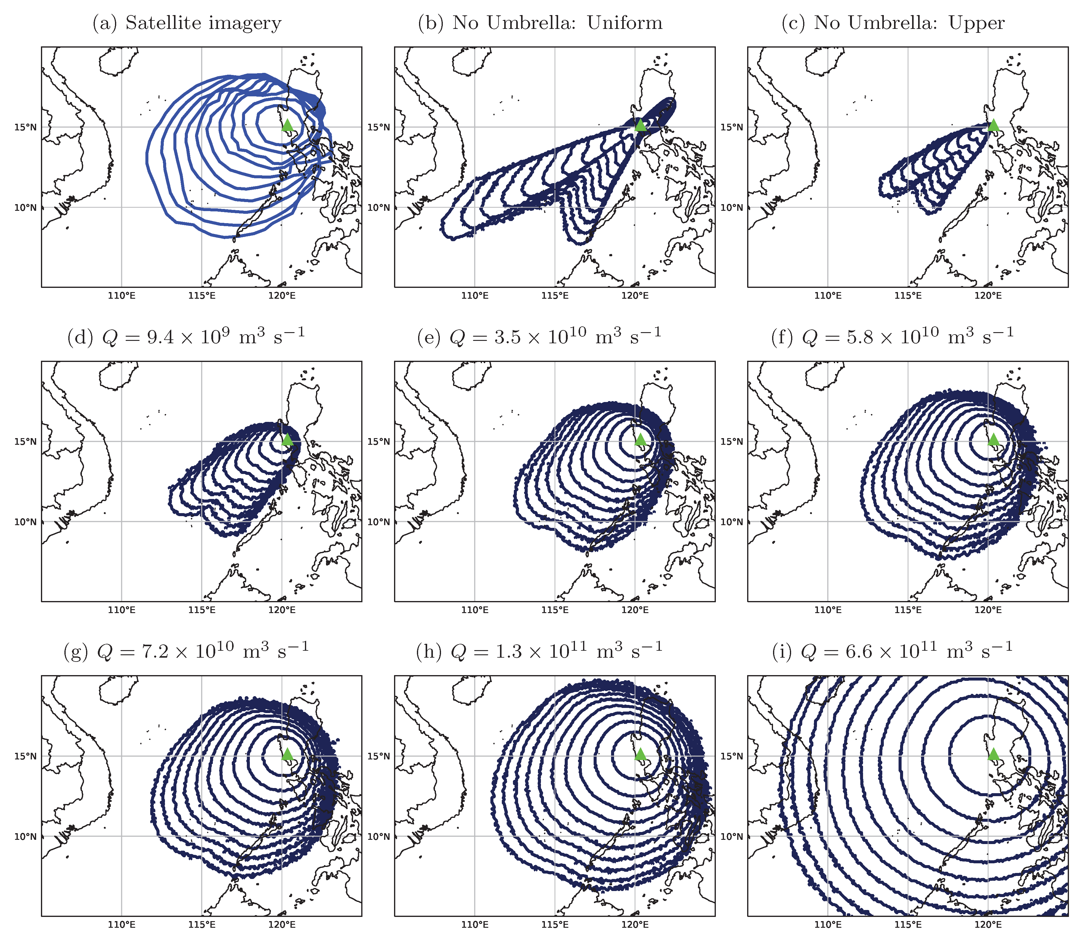
The underprediction of radial spread has been addressed in modelling activities in a variety of ways. In some cases, the horizontal extent of the ash-cloud source within the VATDM has been adjusted to account for the lateral spread. Based on satellite imagery of the Pinatubo ash cloud at 08:41 UTC on 15 June 1991, Witham et al. [6] used a cylindrical ash source with a diameter of 550 km. The ash cloud in the initial hours of the climactic phase was not modelled and subsequent transport and dispersion was assumed to be passive, with radial velocities within the umbrella cloud neglected. This simplified approach did not, however, accurately represent the subsequent spread of the ash cloud [
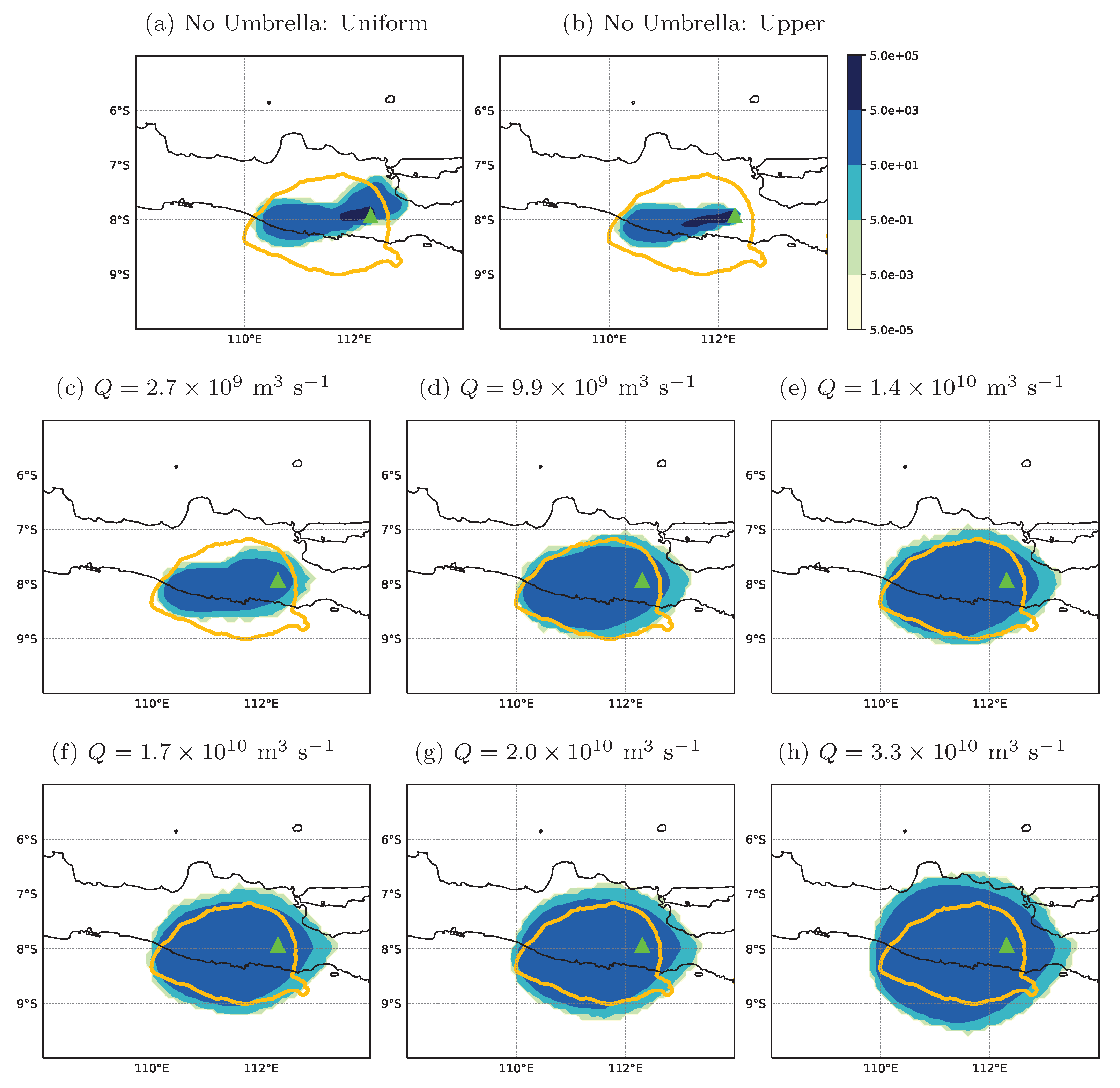
6]. In a similar way, whilst using an inversion method to determine the altitude of the February 2014 Kelud ash cloud, Zidikheri et al. [7] assumed a cylindrical source with a diameter based on the size of the umbrella cloud seen in satellite imagery. The horizontal extent of the modelled source was used once again to account for the radial spread within the umbrella cloud. Alternative strategies involve representing the lateral spread within the VATDM. In some studies, diffusion within the model has been adjusted to match the observed spread of the ash cloud [8]. A wide range of diffusion coefficients is expected, with different values required at different times and for different eruptions, and large diffusion coefficients needed to represent the lateral spread of umbrella clouds. A different strategy is to add, to the VATDM, an explicit parameterisation of lateral spread within the umbrella cloud. Recent work by Costa et al. [4] and Mastin et al. [5] has developed representations of umbrella cloud intrusions for the Eulerian models FALL3D and Ash3d, respectively. In these parameterisations, a radial wind field is applied within the modelled umbrella cloud region, alongside the ambient mean wind field.
The London VAAC uses the Lagrangian dispersion model NAME (Numerical Atmospheric-dispersion Modelling Environment [9]), which hitherto has not explicitly represented lateral spreading within umbrella clouds. Any accounting for umbrella clouds formed during large eruptions would have been guided by observations and required manual adjustments to the VATDM forecasts. We describe here a parameterisation of lateral spreading within umbrella clouds that has recently been added to NAME (version 8.0) and which is designed to be used in an operational context when information on the eruption may be limited and model runtime is key. Section 2 and Section 3 describe the formation of umbrella clouds, the governing equations for the lateral spread and the implementation of these equations into NAME. In Section 4, we discuss the input parameters required by the parameterisation. The eruptions of Pinatubo in 1991, Kelud in 2014, Calbuco in 2015 and Eyjafjallajökull in 2010 are used to validate the parameterisation of lateral spread, as presented in Section 5. These case studies represent eruptions of differing scales and are well observed by satellite. The satellite observations are available in various forms (e.g., brightness temperatures or retrievals of ash column loads), reflecting the different sources of this observational data. Nonetheless, all forms of satellite data used are suitable for indicating the observed lateral spread of the umbrella cloud, since the edge of the cloud is characterised by sharp gradients in ash column loads or sudden drop-offs in brightness temperatures. The paper ends with a discussion of various issues in Section 6 and conclusions are drawn in Section 7.

2. Umbrella Cloud Dynamics

During explosive eruptions, the ejected volcanic material is rich in solid ash particles with a density much greater than that of the surrounding atmosphere. Entrainment of ambient air into the hot volcanic plume can reduce the plume density drastically, leading to a buoyant eruption column. Strong plumes from explosive eruptions can rise above the tropopause, forming a vertical eruption column. At the level of neutral buoyancy ( H N B L ), the density of the rising ash plume is the same as that of the surrounding atmosphere and the plume is no longer buoyant. The plume continues to rise due to its momentum but, since it is now denser than its surroundings, it decelerates and the overshooting plume finally reaches its maximum height ( H T ). The plume material then begins to slump back down due to gravity, forming an intrusive gravity current which spreads laterally in an expanding umbrella cloud. Due to continued entrainment, the height of the umbrella cloud intrusion lies somewhere between the initial level of neutral buoyancy ( H N B L ) and the overshooting plume top ( H T ).

3. The Umbrella Cloud Scheme

Equations governing the growth rate of the umbrella cloud are derived from conservation laws in two ways. Sparks et al. [3], Costa et al. [4] and Mastin et al. [5] assumed an expanding cylindrical umbrella cloud with time-varying radius R = R ( t ) and depth h ¯ = h ¯ ( t ) (the average depth of the umbrella cloud at time t), where t is the time since the start of the eruption/umbrella cloud formation. By conservation of volume,
d d t π R 2 h ¯ = Q ,
where Q is the volume flow rate of material (gas and ash) into the umbrella cloud. Conversely, Woods [10] and Rooney and Devenish [11] considered a non-cylindrical shape with depth h R = h R ( t ) at the leading edge. Assuming there is no change in shape to the already-formed umbrella cloud,
2 π R u R h R = Q ,
by conservation of volume flux, where u R is the speed of the leading edge of the umbrella cloud. In both derivations, entrainment within the umbrella cloud region is neglected and the eruption is assumed to be steady. Based on results from models and experiments [10,11], the velocity of the leading edge of the umbrella cloud ( u R ) is assumed to scale linearly with the cloud depth,
u R = d R d t = λ N h ¯   or   u R = d R d t = F N h R ,
where N is the buoyancy frequency of the atmosphere at the height of the intrusion and λ and F are empirical constants of order unity [3,4,11]. Substituting for h ¯ or h R using Equation (3) and integrating Equation (1) or (2), one obtains
R = 3 λ N Q 2 π 1 / 3 t 2 / 3 = 3 2 2 / 3 F N Q 2 π 1 / 3 t 2 / 3 ,
for R R ( 0 ) . The speed of the umbrella cloud front u R is given by
u R = 2 3 3 λ N Q 2 π 1 / 2 R 1 / 2 = F N Q 2 π 1 / 2 R 1 / 2 .
Thus, the end result is the same, with F = 4 λ / 3 .
There is some uncertainty in the value of the constants λ and F with values in the range 0.1–0.6 quoted in the literature [12,13]. Similar values are used within umbrella cloud parameterisations: Costa et al. [4] and Mastin et al. [5] assumed λ = 0.2 , Rooney and Devenish [11] took F = 4 λ / 3 = 0.3 (here, F is the Froude number of the gravity current) and Suzuki and Koyaguchi [14] used large-eddy simulations (LES) to show that λ = 0.2 and λ = 0.1 are suitable values for eruptions in tropical and midlatitude regions, respectively. Here, we follow Rooney and Devenish [11] and take F = 0.3 or λ = 3 F / 4 = 0.225 .
In line with other implementations of an umbrella cloud parameterisation [4,5], we compute a time-dependent radial velocity field centred above the volcano vent. The radial velocity at the leading edge of the umbrella cloud, u R , is given by Equation (5). Within the umbrella cloud interior ( r < R , where r is the radial distance), Costa et al. [4] determined the radial velocity u ( r ) from
u ( r ) = 3 4 u R R r 1 + 1 3 r 2 R 2 ,
where u R is given by Equation (5). The derivation of Equation (6) assumes a cylindrical umbrella cloud, the height of which h ¯ ( t ) varies with time. Consider, for a moment, a point at a fixed distance r from the umbrella cloud centre and analyse the radial velocity u ( r ) at this point. If r R , then u ( r ) R 1 / 2 / r in Equation (6) and u ( r ) increases with time (along with R), reaching its maximum value at the end of the eruption. This maximum value depends on the size of R and can be large for sustained eruptions or for eruptions with giant umbrella clouds.
In the scheme presented here, we extrapolate Equation (5) to 0 < r < R , namely
u ( r ) = 2 3 3 λ N Q 2 π 1 / 2 r 1 / 2 .
Here, u ( r ) r 1 / 2 throughout the umbrella cloud, which, for r R , gives substantially lower radial velocities than Equation (6). Equation (7) can be viewed as assuming a steady flow field, where u ( r ) is constant with time for a fixed r when r R ( t ) . Both Equations (6) and (7) give the required radial velocity at the leading edge ( r = R ) as given by Equation (5). Hence, the rate of growth of the umbrella cloud will be the same under this parameterisation and that of Costa et al. [4] (note the use of Equation (5) for u R in both) but with differences within the umbrella cloud in the rate of outward radial transport, and in the resulting distribution of ash.
In Lagrangian models, large numbers of “model particles”, representing the emission of material (here, volcanic ash), are advected within the model atmosphere due to the mean ambient wind, atmospheric turbulence and, if appropriate, gravitational settling. Within the umbrella cloud, model particles are also advected by the radial velocity u ( r ) . Equation (7) is integrated to compute a radial increment, Δ r , at each time-step, Δ t ,
Δ r = r ( t + Δ t ) r ( t ) = 3 λ N Q 2 π 1 / 2 Δ t + r ( t ) 3 / 2 2 / 3 r ( t ) .
This avoids issues with large radial velocities near to the vent in Equation (7), which, with Δ r = u ( r ) Δ t , would require small model time-steps. Within the umbrella cloud region (i.e., for r ( t ) R ( t ) , where R ( t ) is given by Equation (4)), this radial increment is added to the model particle’s advection alongside components due to transport by the mean ambient wind and turbulence. Outside the umbrella cloud, i.e., for r > R , u ( r ) is commonly assumed to be zero [5]. This gives a discontinuity in the radial velocity, changing from u R to zero at the leading edge of the umbrella cloud. Lagrangian models are, however, prone to particle accumulation issues in regions with such step changes (see Appendix A). Consequently we employ a soft boundary instead, in which u ( r ) 0 for r > R , namely we make the pragmatic choice
u ( r ) = u R R r 5 = 2 3 3 λ N Q 2 π 1 / 2 R 1 / 2 R r 5 .
Within the Lagrangian model, there is a trade-off between the rate at which the radial velocity tends to zero outside of the umbrella cloud (to minimise excessive transport on the downwind edge) and the amount of particle accumulation at the leading edge. Sensitivity tests suggest that u ( r ) r 5 (as in Equation (9)) gives the required rapid decrease in the radial velocity outside the umbrella cloud, without undue amounts of particle accumulation resulting in large unrealistic increases in predicted total ash column loads or ash concentrations at the leading edge. Integrating Equation (9) gives the (suitably small) radial increment applied outside the umbrella cloud
Δ r = r ( t + Δ t ) r ( t ) = R ( t + Δ t ) 6 R ( t ) 6 + r ( t ) 6 1 / 6 r ( t ) .
The implementation of radial spreading alongside transport and dispersion due to the ambient mean wind and turbulence ensures that the appropriate behaviour is predicted. For large radial velocities, lateral spreading will dominate the transport and dispersion, with upwind transport of the ash cloud and near-circular cloud growth. The ash cloud reaches a stagnation point upwind when the radial velocity and atmospheric wind velocity are equal in magnitude but opposite in direction. The parameterisation is required, however, to be well-behaved for smaller eruptions, having minimal effect when transport and dispersion are dominated by the mean ambient wind and atmospheric turbulence. There may be scope to improve the scheme for eruptions in which radial velocities within the umbrella cloud are comparable in size to ambient velocities. The simple addition of velocity fields used here may not be as appropriate in these cases.
Despite the implementation of the scheme requiring the volume flow rate into the umbrella cloud to be constant (i.e., steady), it does allow non-umbrella cloud sources without radial spreading (e.g., from different phases of the eruption or ash released from lower levels in the eruption column) to be independently modelled alongside an umbrella cloud, if required, or, indeed, multiple distinct umbrella clouds from different eruptive phases (and with differing volume flow rates) to be represented. In line with other umbrella cloud parameterisations [4,5], radial spreading is terminated as soon as the eruption ceases. Furthermore, mass conservation requires that the umbrella cloud thins as it expands over time but parameterisations do not include this thinning. Vertical transport within the modelled umbrella cloud is due solely to the ambient mean wind, turbulence and gravitational settling.
We note that Pouget et al. [15] proposed alternative umbrella cloud growth rates within different flow regimes. Using the intrusion model developed by Johnson et al. [16], which solves a system of “shallow-water” equations, and comparing the modelled umbrella cloud growth with that observed by satellite, Pouget et al. [15] showed a transition between a buoyancy-inertial regime, where the dominant force resisting spreading is the inertia of the displaced fluid (inertial drag), and a turbulent drag-dominated regime late in the spread, where the buoyancy forces have decreased and the dominant resisting force is the drag along the cloud interfaces. For long-lived eruptions, the growth of the umbrella cloud was found to tend to R ( t ) t 3 / 4 in the buoyancy-inertial regime and R ( t ) t 5 / 9 in the turbulent drag regime. Pouget et al. [15] noted that the growth rate approaches this asymptotic behaviour at large time and, for a given time, the flow may not be fully in any particular regime. The exponent of t will therefore vary with time. The growth rate used in our scheme (Equation (4): R ( t ) t 2 / 3 ) is not too dissimilar to that found by Pouget et al. [15], particularly since, as noted above, the flow could be adjusting towards the asympototic behaviour. For short-lived eruptions, Pouget et al. [15] found much smaller rates of growth: R ( t ) t 1 / 3 in the buoyancy-inertial regime and R ( t ) t 2 / 9 in the turbulent drag regime.

4. Estimating Umbrella Cloud Parameters

Within the umbrella cloud scheme in NAME, volcanic ash is released over a finite layer at the height of the intrusion. The depth of this modelled ash layer is expected to be greater than the depth of the umbrella cloud since it represents uncertainty in the intrusion height. Except for the largest, and most rapidly expanding, umbrella clouds, the model predicted ash cloud extent and position is sensitive to the height and depth of this modelled ash layer when there is significant atmospheric wind shear.
The volume flow rate into the umbrella cloud (Q) and the intrusion height are inputs required by the scheme. In an operational setting, details of the eruption may be scarce. Consequently, these input parameters may need to be estimated from limited available observations. Simple empirical formulae (as described below) can be used or 1D and 3D plume models can be run.
Plume heights are often reported during an eruption by the local volcano observatory. For example, during Icelandic volcanic eruptions, the London VAAC receives regular reports from the Icelandic Meteorological Office (IMO). These reports include plume height information, which is based on radar measurements and other observations. The plume height measured by the radar is subject to uncertainties due to discrete scanning angles. Furthermore, certain meteorological conditions can lead to additional uncertainties if the plume top is not within view. For example, the viewing perspective may obscure the plume top if, due to the ambient wind, the maximum plume height occurs some distance downwind. In this case, the observed plume top may not be the maximum plume height. Estimates of the ash cloud height can also be determined from satellite observations, for example by comparing observed brightness temperatures with atmospheric profiles [17,18] or by performing a 1D variational retrieval [19,20]. These satellite derived ash plume heights are also subject to uncertainties, particularly for large stratospheric eruptions when the temperature of the overshooting plume top can be significantly colder than the ambient temperature. Alternative plume height measurement techniques include visual observations and other indirect methods, such as estimating plume heights from ash deposits [21,22]. A summary of methods for determining ash cloud heights is given in Taylor et al. (Table 1 in [23]). For all plume height measurements, however, it is important, for modelling purposes, to understand if the reported height refers to the maximum height reached by the overshooting plume or to the height of the atmospheric intrusion of ash.

4.1. The Umbrella Cloud Intrusion Height

The height of the intrusion is generally lower than the overshooting plume top but above the level of neutral buoyancy of the rising plume (although, for simplicity, it is common to assume that the height of the umbrella cloud and the level of neutral buoyancy are approximately the same). If observations of the intrusion height are available (for example, from visual observations or derived from satellite observations or from distributions of ash deposits), this height information can be input directly by the user and would then be used within the model to govern the elevation of the release of ash into the umbrella cloud.
If observations of the height of the umbrella cloud are not available, then an estimate is obtained from the maximum plume height ( H T ). (Note that H T , together with all other height definitions (e.g., H N B L ), refers, in this paper, to height above vent level (avl).) In the 1D fluid dynamics and thermodynamics model of Morton et al. [24], developed for simple single-phase Boussinesq plumes in a linearly stratified environment, the height of the eruption column ( H T ) and the height of the level of neutral buoyancy ( H N B L ) are given by
H T = C 1 k 1 / 2 F 0 1 / 4 N 3 / 4 ,
H N B L = C 2 k 1 / 2 F 0 1 / 4 N 3 / 4 ,
where C 1 and C 2 are constants of proportionality, k is an entrainment constant, F 0 is the “initial” buoyancy flux and N is the Brunt–Väisälä frequency of the atmosphere [14,24]. The driving force for the umbrella cloud depends on H T H N B L , which is proportional to H T . Likewise, the ratio of the two plume heights ( H N B L / H T ) is constant ( C 2 / C 1 ). In a similar way, we assume that the height of the umbrella cloud ( H U ) can be estimated according to
H U = C H T ,
where the value of the constant of proportionality (C) is based on results from large-eddy simulations and numerical plume models [11,14], observations from previous eruptions and other information in the literature, as detailed in Table 1.
Suzuki and Koyaguchi [14] used a 3D model to simulate explosive eruptions generating large-scale umbrella clouds in both tropical and midlatitude atmospheres. From the simulations, the maximum ash column height ( H T ), the altitude of the level of neutral buoyancy of the rising column ( H N B L ) and the altitude of the umbrella cloud ( H U ) are determined. H U is systemically higher than H N B L due to further entrainment of ambient air above the level of neutral buoyancy. The ratios of H U / H T and H N B L / H T obtained from their simulations of eruptions on the scale of the climactic phase of the 1991 eruption of Pinatubo, in both tropical and midlatitude atmospheres, are quoted in Table 1.
Similar results are obtained from other models. Mastin [26] presented simulations using the 1D plume model Plumeria [27] in both dry and wet atmospheres. The mean and standard deviation of the ratios H U / H T and H N B L / H T are given in Table 1. Large-eddy simulations by Devenish et al. [25] are compared by Rooney and Devenish [11] to results from other models [24,28,29]. Table 1 shows the ratio of H U / H T and H N B L / H T from all results presented by Rooney and Devenish [11].
Data from three historic eruptions which led to umbrella cloud formation are also included. The ratio H U / H T is derived from the following assumed values: Pinatubo—the maximum plume height is 37 km avl and the height of the umbrella cloud is 25 km avl [4,5,12]; Kelud—the overshooting plume top is 26 km asl (above sea level), the umbrella cloud height is 19 km asl and the vent is 1.731 km asl [
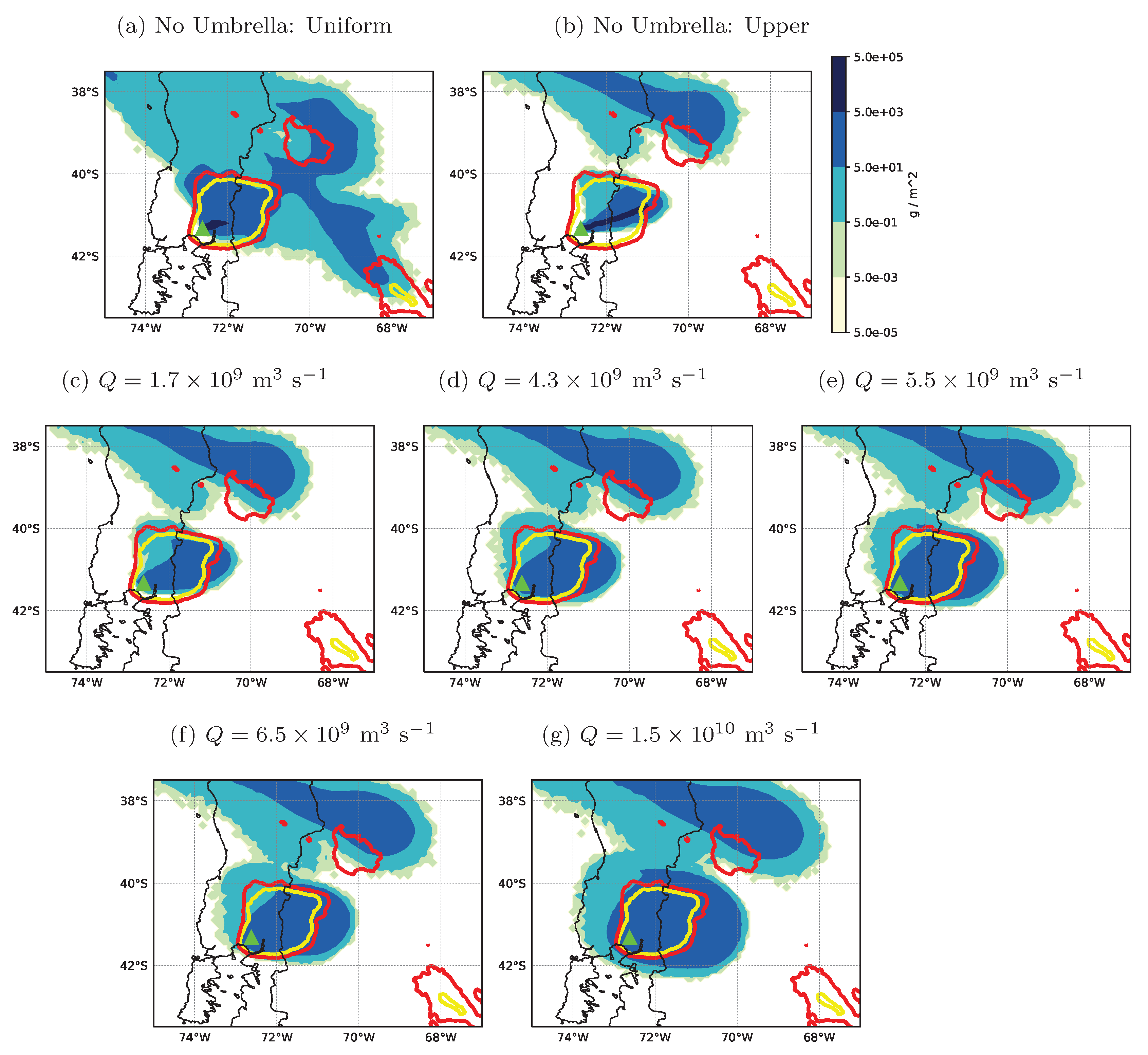
30]; and Calbuco—the maximum plume height is 23 km asl, the height of the umbrella cloud is 17 km asl and the vent is 2.003 km asl [31,32].
When information on the height of the umbrella cloud is not available, we assume, based on the data in Table 1, a modelled source with a top at a height 0.8 H T and a base at a height 0.65 H T . This gives an elevated release of ash within a layer with depth 0.15 H T which spans most of the umbrella cloud heights given in Table 1. Ash is only released within this layer, using a uniform vertical distribution. The mass release rate within the model represents only the fine ash fraction which survives near source fallout and is therefore typically not related to the lateral spreading rate of the umbrella cloud or estimates of the volume flow rate (see Section 5 for more details).

4.2. The Volume Flow Rate into the Umbrella Cloud

An estimate of the volume flow rate into the umbrella cloud (Q) is also required and this governs the rate at which the ash cloud spreads laterally within the model. Observations can be used to determine Q. This includes a simple method of estimating Q from observations of the maximum plume height.
The growth rate of the umbrella cloud can be obtained from a time sequence of satellite images [32]. Using Equation (4) and the umbrella cloud radius (R) determined from satellite imagery at two different times ( R ( t 1 ) and R ( t 2 ) ), Q can be estimated. The estimated Q is an average value over the time period [ t 1 , t 2 ]. Erupted mass estimates, obtained, for example, from mapped deposits, can also be used to calculate volume flow rates from average mass eruption rates [5,32].
In the initial stages of an eruption, mapped deposits and long sequences of satellite imagery of the ash cloud will not be available. An estimate of Q can, however, be made based on the maximum height of the ash plume ( H T ). In the 1D model of Morton et al. [24], the volume flow rate is given by
Q = C 3 k 1 / 2 F 0 3 / 4 N 5 / 4 ,
where C 3 is a constant of proportionality and k, F 0 and N are as defined in Equation (11). Eliminating F 0 using Equation (11), one obtains a relationship between H T and Q, namely
Q = C 3 C 1 3 k 2 N H T 3 ,
where the ratio of the constants of proportionality can be determined from plume models and large-eddy simulations. Using an entrainment coefficient value k = 0.085 , Rooney and Devenish [11] obtained Q / ( N H T 3 ) = C 3 k 2 / C 1 3 = 9.29 × 10 3 from the large-eddy simulations of Devenish et al. [25]. From the results of the 3D plume model simulations by Suzuki and Koyaguchi [14], larger values of Q / ( N H T 3 ) = C 3 k 2 / C 1 3 are obtained: between 0.035 and 0.071 (for simulations in a tropical atmosphere) and between 0.023 and 0.078 (for simulations in a midlatitude atmosphere). Suzuki and Koyaguchi [14] estimated effective values for the entrainment coefficient k, with k = 0.1 in tropical atmospheres and for relatively small-scale eruptions in midlatitude atmospheres, and with k < 0.07 for large-scale eruptions in midlatitude atmospheres. These model simulations indicate that there is some uncertainty in the constants in Equation (15), which, in turn, translates into significant uncertainty in the estimated volume flow rates (as shown in Section 5).
Bursik et al. [33] gave an approximate relationship between Q (in m 3 s 1 ) and H T (in m avl),
Q = H T 287 1 / 019 ,
which is derived from fitting an empirical equation to numerical results. We show in Section 5 that the predicted lateral spread, obtained from the umbrella cloud scheme using volume flow rates estimated from this empirical equation, agrees reasonably well with observations for a wide range of scales of eruptions.

5. Validation

Here, we compare NAME model predictions of the spread of the volcanic ash cloud with satellite imagery from four historic eruptions of differing scales: Pinatubo in 1991, Eyjafjallajökull in 2010, Kelud in 2014 and Calbuco in 2015. Table 2 details the input NWP meteorological data used in the NAME simulations. Model runs are conducted with and without the umbrella cloud parameterisation. Without the umbrella cloud parameterisation, two source options are assessed: the default London VAAC setup which releases ash uniformly from the volcano vent to the maximum plume height H T (hereafter labelled “Uniform”) and a release of ash within an elevated layer (labelled “Upper”). Note that the “Upper” simulations use an identical source term as the umbrella cloud simulations, with ash released uniformly within an elevated layer of depth 0.15 H T and with the top of the layer at the known height of the umbrella cloud top. The modelled mass release rate is calculated independently of the volume flow rate and is obtained for each eruption from H T using the empirical equation of Mastin [26]. Only the fine ash fraction which does not deposit near the source is modelled and this is assumed to be 5% of the Mastin [26] value. The default particle size distribution used within NAME by the London VAAC for volcanic ash particles in the size range 0.1–100 μ m diameter is adopted [34].
The model simulations for each eruption are presented in turn and the results are then summarised.

5.1. Pinatubo

The climactic phase of the 1991 eruption of Mount Pinatubo ( 15.13 N, 120.35 E) began at 04:40 UTC on 15 June 1991 and resulted in an ash column reaching a height of almost 40 km. A large umbrella cloud formed (see Figure 1a), expanding radially over an area of more than 1000 km in diameter in less than 11 h [12]. Large radial velocities, up to 20 m s 1 , within the umbrella cloud resulted in significant upwind spread.
For modelling the climactic phase, we assume an overshooting plume top of 37 km avl [4,12]. In line with other modelling studies of the Pinatubo eruption, which revealed inconsistencies between satellite imagery of the ash cloud and the reanalysis NWP wind direction [4,5], we rotate the ERA-Interim wind fields anticlockwise by 30 degrees. Following Costa et al. [4] and Mastin et al. [5], we take N = 0.02 s 1 and assume a 9 h release with an umbrella cloud top at 25 km asl, in agreement with Geostationary Meteorological Satellite (GMS) observations [12].
The outline of the observed umbrella cloud at hourly intervals starting at 05:40 UTC on 15 June 1991 is shown in Figure 1a [12]. Corresponding predicted ash clouds obtained from NAME simulations are shown in Figure 1b–i. Model simulations without representing the lateral spread within the umbrella cloud are shown in Figure 1b,c. In Figure 1b, a uniform release between the vent and 37 km avl is represented. (The vent is taken to be 1.7455 km asl.) The “Upper” simulation in Figure 1c uses a uniform release over an elevated layer with a vertical extent of 5.55 km and a top at 25 km asl, corresponding to the umbrella cloud top observed in satellite images.
Figure 1d–i shows NAME model predictions using the umbrella cloud parameterisation with different estimates of Q (as given in Table 3) and an umbrella cloud top at 25 km asl. Figure 1f uses an average volume flow rate of Q = 5.8 × 10 10 m 3 s 1 determined by Mastin et al. [5] from estimates of the erupted volume. In comparison, Costa et al. [4] subdivided the climactic phase into three intervals: (i) 04:40–07:10 UTC with an eruption height of 37 km avl and a volume flow rate of 1.29 × 10 11 m 3 s 1 ; (ii) 07:10–11:40 UTC with an eruption height of 31.5 km avl and a volume flow rate of 9.5 × 10 10 m 3 s 1 ; and (iii) 11:40–14:40 UTC with an eruption height of 26 km avl and a volume flow rate of 3.7 × 10 10 m 3 s 1 . The largest estimated volume flow rate into the Pinatubo umbrella cloud in Table 3 is 6.56 × 10 11 m 3 s 1 and is obtained using the plume model of Devenish [35], assuming a plume height of 37 km avl. This plume model includes the effects of moisture and the ambient wind. Other estimates in Table 3 of the volume flow rate into the Pinatubo umbrella cloud are determined using Equations (15) and (16), assuming H T = 37 km and N = 0.02 s 1 .

5.2. Kelud

An explosive eruption of the Kelud volcano ( 7.93 S, 112.308 E) occurred at 15:50 UTC on 13 February 2014. The initial lateral blast was followed by a brief pause before a short-lived (<3 h) explosive eruption resulted in a stratospheric ash plume and the formation of an umbrella cloud. Satellite imagery indicated an overshooting plume top reaching a height exceeding ∼26 km and a rapidly expanding umbrella cloud with a top around 18–19 km asl [30]. From analysis of the growth rate of the umbrella cloud, Hargie et al. [36] determined that the emission of ash for this phase of the eruption began ∼16:09 UTC.
For modelling the eruption of Kelud on 13 February 2014, we assume an overshooting plume top of 26 km asl [30]. We take N = 0.02 s 1 and assume a release from 16:09 to 18:59 UTC with an umbrella cloud top at 19 km asl, in line with satellite observations [30].
Figure 2 compares NAME model simulations of the February 2014 Kelud ash cloud with satellite data at 18:19 UTC from MTSAT geostationary satellites. Model simulations without representing the lateral spread within the umbrella cloud are shown in Figure 2a,b. In Figure 2a, a uniform release between the vent and 26 km asl is represented. (The vent is taken to be 1.731 km asl.) The “Upper” simulation in Figure 2b uses a uniform release within a layer with a vertical extent of 3.54 km and a top at 19 km asl, corresponding to the umbrella cloud observed in satellite images.
Figure 2c–h compares satellite observations, of the Kelud umbrella cloud at 18:19 UTC on 13 February 2014, with NAME model predictions obtained using the umbrella cloud parameterisation with different estimates of Q (as given in Table 3) and an umbrella cloud top at 19 km asl. Figure 2f uses an average volume flow rate obtained from the umbrella cloud expansion rate determined from satellite imagery [36] and assuming N = 0.02 s 1 . Other estimates of Q are obtained using the plume model of Devenish [35] and Equations (15) and (16) with N assumed to be 0.02 s 1 and H T = 24.269 km avl.

5.3. Calbuco

The eruption of Calbuco volcano ( 41.33 S, 72.618 W) in southern Chile on 22 and 23 April 2015 occurred with little warning. Two explosive phases occurred in the initial stages of the eruption, with maximum plume heights of at least 23 km asl recorded by weather radar [31]. The ash cloud was transported north-eastwards and observed by satellite. Phase 1 began at 21:04 UTC on 22 April 2015 and ended at 22:35 UTC. Phase 2 began a few hours later at 03:54 UTC on 23 April 2015 and ended at 10:00 UTC, with a drop in activity sometime between 05:38 and 06:38 UTC. The height of the umbrella clouds were reported to be 14.5–15.5 km asl (Phase 1) and 16.9–17.3 km asl (Phase 2) [32].
Fall deposits were analysed and used to obtain mass eruption rates and total bulk volume estimates of ash [32]. These estimates could be used to infer the volume flow rate into the umbrella cloud. Here, we use, instead, umbrella cloud expansion rates calculated by Van Eaton et al. [32] from infrared images from the GOES-13 satellite. Using Equation (4), a calculated buoyancy frequency of 0.014 s 1 and λ = 0.2 , Van Eaton et al. [32] obtained volume flow rate estimates from the observed umbrella cloud expansion rates. The estimated volume flow rates for both phases are given in Table 3. The buoyancy frequency used by Van Eaton et al. [32] is an average atmospheric value over the eruption column, calculated as described in Equation (10) of Mastin [26]. The value of N required in Equation (4) is, however, the atmospheric value at the level of the intrusion which, for large stratospheric eruptions, is expected to be approximately 0.02 s 1 . Using N = 0.02 s 1 , the observed lateral spread can be obtained with slightly lower estimates of the volume flow rate: Q = 3.9 × 10 9 m 3 s 1 for Phase 1 and 5.5 × 10 9 m 3 s 1 for Phase 2. (Note that the assumed value of λ also contributes some uncertainty to the estimated Q.) The precise value of Q is, of course, only relevant for comparing the estimated volume flow rate to other estimates. Provided that the product λ N Q has the required value, the correct lateral spread will be predicted by the model.
For modelling the two phases of the eruption of Calbuco on 22 and 23 April 2015, we assume an overshooting plume top of 23 km asl [31,32]. We take N = 0.02 s 1 and assume a release during 21:04–22:34 UTC on 22 April 2015 with an umbrella cloud top at 16 km asl for Phase 1 and, for Phase 2, a release during 04:00–10:00 UTC on 23 April 2015 with an umbrella cloud top at 17 km asl. We assume a steady eruption throughout each phase.
Figure 3 compares NAME model simulations of the ash cloud from the two-phase eruption of Calbuco in April 2015 with satellite data from GOES-13 at 07:08 UTC on 23 April 2015. Figure 3a,b shows model simulations without representing the lateral spread within the umbrella cloud. In Figure 3a, a uniform release between the vent and 23 km asl is represented. (The vent is taken to be 2.003 km asl.) The “Upper” simulation in Figure 3b releases ash within an elevated layer, with a vertical extent of 3.15 km (both phases) and a top at 16 km asl for Phase 1 and at 17 km asl for Phase 2. There is an offset in the downwind position of the satellite observed and model predicted ash cloud from Phase 1. Van Eaton et al. [32] estimated that the observed ash clouds from GOES-13 were displaced approximately 15 km south, due to parallax from the oblique view of the satellite, but without any substantial distortion of their shape or area. This only partially accounts for the discrepancy in the downwind location of the observed and modelled ash cloud from Phase 1 and errors in the modelled ash cloud must also exist. These “modelling errors” may be inaccuracies in the timing or height of the ash release, or errors in the input meteorological data.
Figure 3c–g compares satellite observations to NAME model predictions obtained using the umbrella cloud parameterisation with different estimates of Q (as reported in Table 3). There is a disagreement in the orientation of the ash cloud from Phase 2, with the modelled cloud from Phase 2 heading northeastwards and the observed ash cloud heading in a more northerly direction. Atmospheric wind shear is evident in this case and the downwind direction is strongly influenced by the ash release height. The discrepancy in the orientation of the ash cloud may be indicative of a slight error either in the NWP model winds or in the height and/or depth of the modelled umbrella cloud. Better agreement is obtained if the umbrella cloud top for Phase 2 is assumed to be approximately 19–20 km asl. Figure 3e uses an average volume flow rate determined (as described above) from the umbrella cloud expansion rate obtained from satellite observations by Van Eaton et al. [32]. Other estimates of Q are obtained using the plume model of Devenish [35] and Equations (15) and (16) with N assumed to be 0.02 s 1 and H T = 21.997 km avl.

5.4. Eyjafjallajökull

It is important that the umbrella cloud parameterisation is well behaved for all scales of eruptions, representing well the lateral and upwind spread within umbrella clouds formed during large explosive eruptions and, at the same time, having negligible effect for small scale eruptions. The scale of the eruption of the Icelandic volcano Eyjafjallajökull ( 63.63 N, 19.62 W) in April and May 2010 was relatively small, with no reports of umbrella cloud formation and maximum plume heights up to 10 km asl. To assess the performance of the umbrella cloud parameterisation for such small-scale eruptions, we study a period in early May when explosive activity began to increase again and the resulting ash cloud was well observed by satellites.
For simulating this period of the eruption of Eyjafjallajökull, we model an overshooting plume top of 10 km asl starting at 18:30 UTC on 5 May 2010 [34]. The vent is taken to be 1.666 km asl. As no umbrella cloud formation was reported, we use an elevated layer estimated by default from H T by the parameterisation, namely ash is released uniformly between 7.083 and 8.333 km asl. For small eruptions without an overshooting plume, the user could choose to set the “umbrella cloud top” to the maximum plume height, thereby releasing ash in a layer at the top of the plume. We take, as before, N = 0.02 s 1 , although we note that, for this tropospheric eruption, this may be a little too large and consequently the predicted lateral spread may be overdone.
Figure 4 compares NAME model simulations of the Eyjafjallajökull ash cloud at 13:00 UTC on 6 May 2010 with SEVIRI satellite data. Differences between the modelled ash clouds in the simulations are very small (cf. Figure 4a–g). We note that the modelled ash clouds are transported further downwind from the source than the ash cloud observed by SEVIRI. This may be because atmospheric cloud was obscuring the ash cloud, some atmospheric ash was below levels detectable by SEVIRI or, alternatively, the release of ash from this phase of the eruption either began later than 18:30 UTC or occurred lower in the atmosphere where wind speeds were less.
Figure 4a,b shows model simulations in which the lateral spread of any umbrella cloud is not represented. Figure 4a has a uniform release of ash from the vent to 10 km asl, and, in Figure 4b, an elevated release between 7.083 and 8.333 km asl is used. The NAME model predictions in Figure 4c–g are obtained using the umbrella cloud parameterisation with different estimates of Q (as given in Table 3). The estimated volume flow rates into the “umbrella cloud” are small in comparison to the other eruptions studied and are obtained assuming H T = 8.334 km avl (10 km asl). Similarities between the NAME predicted ash clouds in Figure 4a–g indicate that transport and dispersion by the atmospheric mean wind and turbulence dominates here. Furthermore, these plots suggest that precise estimates of the volume flow rate and the buoyancy frequency of the atmosphere at the ash injection level are not important for eruptions on this scale.

5.5. A Summary of the Simulation Results

For large umbrella-cloud-forming eruptions, model simulations without representation of the umbrella cloud dynamics do not capture the observed radial spread of the ash cloud. In these simulations, transport of the predicted ash cloud is primarily governed by the atmospheric winds and the ash release height. There are noticeable differences between the “Uniform” and “Upper” simulations due to the release of ash at different heights in the model atmosphere. For Pinatubo, the “Uniform” simulation (Figure 1b) has more downwind transport than the “Upper” simulation (Figure 1c) (indicative of higher wind speeds aloft) and some upwind spread (signalling a different wind direction at lower levels in the atmosphere). The modelled Kelud ash cloud from the “Uniform” simulation (Figure 2a) has both northeasterly and southwesterly transport (indicative of different wind directions at different levels of the atmosphere), whereas the ash cloud from the “Upper” simulation (Figure 2b) is transported southwesterly from the vent. During the second phase of the Calbuco eruption, atmospheric wind shear is clearly evident, with ash being transported in different directions at different heights. This wind shear produces significant lateral spread in the ash cloud from the “Uniform” release scenario and the modelled ash cloud agrees quite well with satellite observations, despite having no representation of the umbrella cloud dynamics (see Figure 3a). The observed upwind transport of the Calbuco ash cloud is not, however, predicted.
The volume flow rate (Q) into the umbrella cloud increases with the scale of the eruption. Estimated volume flow rates, obtained for a particular eruption using the different methods, vary in excess of an order of magnitude (see Table 3). Model simulations, conducted using the umbrella cloud parameterisation, show that the predicted lateral spread has significant sensitivity to the estimated volume flow rate. Values of Q obtained from observations (for example, from estimates of erupted volume or from analyses of umbrella cloud growth rates) give predicted ash clouds which agree well with satellite observations (see Figure 1f, Figure 2f and Figure 3e). The estimated volume flow rate into the Pinatubo umbrella cloud given by Costa et al. [4] results in an overprediction of the lateral spread of the ash cloud (see Figure 1h). We note, however, that this value of Q applies only for the initial period from 04:40 to 07:10 UTC [4], whereas it has been used here throughout the climactic phase. Costa et al. [4] suggested lower values of Q (and eruption height) after 07:10 UTC but, as implemented in NAME, the umbrella cloud scheme does not allow such a decrease in Q to be represented. Hence, it may be more appropriate to adopt an average volume flow rate over the climactic phase, such as employed by Mastin et al. [5].
The methods used to estimate the volume flow rate into the umbrella cloud from the observed maximum height of the ash plume ( H T ) give a range of values for Q, which lead to significant variation in the radial spread of the ash cloud. The smallest estimates of Q are obtained using Equation (15), with the constant of proportionality determined from the large-eddy simulations described by Rooney and Devenish [11]. Using this estimate of Q, we find that the lateral and/or upwind spread of the umbrella cloud is underpredicted (see Figure 1d, Figure 2c and Figure 3c). The largest values of Q are obtained using the plume model of Devenish [35] and lead to an overestimation in the lateral and upwind spread predicted by the umbrella cloud parameterisation, excessively so for Pinatubo (Figure 1i, Figure 2h and Figure 3g). In an intercomparison exercise of 1D and 3D volcanic plume models, however, mass eruption rates obtained by the plume model of Devenish [35] were found to be in line with rates determined by other models, for strong eruptions similar in scale to Pinatubo in 1991 [37]. The excessive spread seen in Figure 1i may be partly caused by the fact that, as discussed above, the assumed eruption height of 37 km avl is only appropriate for the initial few hours of the climactic eruption.
There is better agreement between satellite observations and model simulations of the ash clouds when the volume flow rate in the umbrella cloud parameterisation is obtained from Equation (15) with the constant of proportionality determined from the 3D plume model simulations in Suzuki and Koyaguchi [14]. For Pinatubo and Kelud, the 3D plume model simulations “T3” and “T1” by Suzuki and Koyaguchi [14], conducted in a tropical atmosphere, are used to give lower and upper estimates, respectively, of the volume flow rate. For Pinatubo, the lower estimate of Q underpredicts the lateral spread of the ash cloud (see Figure 1e), whereas the modelled ash cloud using the upper estimate (Figure 1g) shows good agreement with satellite imagery. We note that the “T1” plume model simulation (used for the upper estimate in Figure 1g) is similar in scale to the 1991 eruption of Pinatubo, with an overshooting plume top of 37.4 km and an umbrella cloud with a height of 23.3 km [14]. For Kelud, we see that the modelled ash clouds using both these lower and upper estimates of Q agree reasonably well with satellite imagery of the umbrella cloud (Figure 2d,g). For Calbuco, the midlatitude 3D plume model simulations “M3” and “M1” [14] are used to obtain lower and upper estimates, respectively, of the volume flow rate. The ash cloud using this upper estimate of Q (Figure 3g) overpredicts the lateral and upwind spread of the umbrella cloud. Conversely, using this lower estimate of Q (Figure 3d), we find that the lateral and upwind spread of the predicted ash cloud region with ash column loads above 5 g m 2 agrees reasonably well with the extent of the satellite brightness temperature contours, aside from the discrepancy in the orientation of the ash cloud.
The volume flow rates estimated using Equation (16) concur with those obtained from other observations (see Table 3). The modelled ash clouds using estimates of Q from Equation (16) agree well with satellite observations for both the Kelud and Calbuco eruptions (Figure 2e and Figure 3f). Compared to the satellite imagery, the lateral and upwind spread of the Pinatubo umbrella cloud in Figure 1h is a little excessive. However, this may be due, at least partly, to modelling a sustained eruption height of 37 km avl throughout the climactic phase. In general, for the three large eruptions studied here, volume flow rates estimated using Equation (16) appear to give the most accurate predictions of lateral spread when only the maximum plume height is known and further information on the volume flow rate is not available. We also observe that the umbrella cloud scheme has minimal effect for modelling small eruptions when transport of the ash cloud is governed by the ambient winds (Figure 4c–g).

6. Discussion

The volume flow rate into the umbrella cloud (Q) is known to govern the rate of lateral spreading and the umbrella cloud scheme introduced into NAME requires this input variable to be specified or estimated. Different ways of obtaining Q from either basic information or more detailed observations have been explored. Estimates of Q vary by at least an order of magnitude (see Table 3). In turn, for large explosive eruptions, the predicted lateral spread has a strong dependency on the estimated volume flow rate, resulting in significantly different ash cloud extents.
In an operational setting, information concerning the eruption is likely to be limited, at least in the initial stages. Consequently, empirical equations to estimate Q from basic information concerning the maximum plume height H T have been tested. Equation (15) is obtained from the 1D integral plume model of Morton et al. [24]. Various plume model and large-eddy simulations from the literature have been used to determine the constant of proportionality. The largest constant of proportionality (and hence the largest estimated volume flow rate from Equation (15)) is derived from a 3D plume model simulation on the scale of the 1991 climactic phase of the eruption of Pinatubo [14]. This estimate of Q results in a good prediction of the lateral spread of the 1991 Pinatubo umbrella cloud. However, we found that the lateral spread of umbrella clouds from smaller scale eruptions is overestimated. Conversely, when the constant of proportionality was derived from smaller scale plume model simulations, the lateral spread of the Pinatubo umbrella cloud was underestimated. In other words, the constant of proportionality in Equation (15) appears to be eruption-scale dependent. Further work is required to explain this but we note that Equation (15) was originally developed for idealised single-phase Boussinesq plumes in linearly stratified environments.
On the other hand, the empirical equation of Bursik et al. [33] (Equation (16)), obtained from a fit to data, was seen to work reasonably well over a wide range of eruption scales, with the increased exponent of H T (which is ∼5 in Equation (16), compared with 3 in Equation (15)) ensuring an increase in Q (and in the lateral spread) for large eruptions but a decrease for small eruptions. For this reason, the operational implementation of the umbrella cloud parameterisation in NAME uses, as default, the Bursik et al. [33] formulation to estimate Q.
The use of 1D volcanic plume models to estimate Q has also been explored. These types of models account for the effects of the ambient wind, moisture, etc. in the ash plume. Relatively large volume flow rates were estimated using the model of Devenish [35] and the subsequent modelled lateral spread of the umbrella cloud was generally overpredicted. Further work is required to understand the large estimates for Q obtained using plume models, particularly for the large-scale eruptions. Coupling an umbrella cloud scheme to a plume model would then be worth exploring at a later date.
We show how additional observations, including mapped deposits and a series of satellite images, can be used, as they become available, to refine estimates of the volume flow rate into the umbrella cloud from an initial first guess and to improve model predictions.
Modelling of the eruption of Calbuco in 2015 highlighted the importance of accurately representing the height of the umbrella cloud within the modelling. Atmospheric wind shear and higher wind speeds aloft can translate errors in the ash release height into errors in the orientation of the modelled umbrella cloud, in the upwind stagnation point and in the distance travelled downwind. Fortunately observations of the umbrella cloud height are often promptly available. However, for situations when this is not the case, we suggest in this paper an ash release height range, based on the maximum plume height H T . Both this emission height range estimate and the method for estimating the volume flow rate from the maximum plume height would, no doubt, benefit from further validation and from testing in an operational context during an eruption.
The parameterisation in its current form assumes a steady eruption in which Q is constant throughout. This has the benefits of a simple and efficient parameterisation. In reality, however, there are likely to be changes in activity over time. Changes to the volume flow rate into the umbrella cloud will result in an adjustment to the growth rate of the umbrella cloud. A limitation of the simple parameterisation implemented here in NAME is that it cannot reproduce this change in behaviour. The change in activity is also likely to be accompanied with a modification to the maximum plume height and potentially to the height of the umbrella cloud. This suggests a complex situation where the injection of ash may or may not feed into the previously formed umbrella cloud. Knowing details of the variation of plume properties over time and developing a parameterisation to make use of this information and to accurately predict the changing behaviour of the growth of the umbrella cloud seems very challenging, particularly in an operational modelling context.
The derivation of the equations determining the rate of lateral spread of the umbrella cloud (Equations (4) and (5)) assumes a thinning of the umbrella cloud depth with time ( d h ¯ / d t or d h R / d t < 0 ). The implementation here does not thin the umbrella cloud over time; there is no vertical motion within the umbrella cloud, aside from the usual components due to the atmospheric mean vertical wind, atmospheric turbulence and gravitational settling. Thinning of the umbrella cloud over time is similarly not included in umbrella cloud parameterisations in other VADTMs [4,5]. This means that the parameterisation is not divergence free and hence ash concentrations within the umbrella cloud may be less accurately predicted than column loads. Modelling the thinning of the umbrella cloud in the NAME parameterisation is the subject of future work.
Aside from all of this, the simple implementation has been seen to be useful in an operational modelling setting, enabling predictions of the position of the ash cloud from large umbrella-cloud-forming explosive eruptions to be greatly improved in a timely fashion.

7. Conclusions

A parameterisation to represent the lateral spread within umbrella clouds has been introduced into the Lagrangian model NAME, resulting in substantial improvements to ash cloud predictions from large explosive eruptions. Results are in good agreement with other umbrella cloud modelling studies using Eulerian models [4,5]. Satellite observations of ash clouds from past eruptions have been invaluable for model validation.
The scheme has been designed for operational use with no impact seen on model runtime. Reasonable model agreement with satellite observations is obtained using only basic information on the eruption to estimate the required input parameters. As more information and observations become available, these input parameters can be refined, leading to improvements in the ash cloud predictions. The scheme has the potential to greatly improve forecasts of the predicted ash cloud location and extent issued by the VAACs during large explosive umbrella-cloud-forming eruptions. Further validation would increase confidence and give a better understanding of performance for different eruptions. Furthermore, testing of the parameterisation during an actual eruption would enable operational forecasters to gain familiarity and see the benefits for themselves.

8. Data Statement

Model output from the NAME simulations appear in the Supplementary Materials to this paper. Satellite retrievals from SEVIRI observations shown in Figure 4 also appear in the Supplementary Materials. For NAME licence enquiries, please contact the Met Office ([email protected]).

Supplementary Materials

Author Contributions

Conceptualisation, H.N.W., L.G.M., B.J.D. and D.J.T.; methodology, H.N.W., B.J.D., D.J.T., L.G.M. and A.R.V.E.; software, H.N.W.; validation, H.N.W.; resources, H.N.W. and A.R.V.E.; writing—original draft preparation, H.N.W.; writing—review and editing, H.N.W., B.J.D., L.G.M., D.J.T. and A.R.V.E.; and visualisation, H.N.W. All authors have read and agreed to the published version of the manuscript.

Funding

This research received no external funding.

Acknowledgments

Use of satellite data processed by Mike Cooke, Met Office (Eyjafjallajökull), and Mike Pavolonis, NOAA/NESDIS (Calbuco/Kelud), is gratefully acknowledged. The authors would also like to thank Antonio Costa (INGV) for helpful discussions on the umbrella cloud equations.

Conflicts of Interest

The authors declare no conflict of interest.

Abbreviations

The following abbreviations are used in this manuscript:
aslabove sea level
avlabove vent level
ECMWFEuropean Centre for Medium-Range Weather Forecasts
GMSGeostationary Meteorological Satellite
GOESGeostationary Operational Environmental Satellite
IMOIcelandic Meteorological Office
MTSATMulti-functional Transport Satellites
NAMENumerical Atmospheric-dispersion Modelling Environment
NWPNumerical Weather Prediction
SEVIRISpinning Enhanced Visible and InfraRed Imager
UTCCoordinated Universal Time
VAACVolcanic Ash Advisory Centre
VATDMVolcanic Ash Transport and Dispersion Model

Appendix A. Particle Accumulation

Lagrangian models are prone to particle accumulation issues in regions with discontinuities in the modelled flow or turbulence field. Figure A1 shows NAME predicted ash column loads within the Pinatubo ash cloud at 09:40 UTC on 15 June 1991 obtained with a step change in the umbrella cloud radial velocity: u ( r ) = u R at r = R (Equation (5)) and u ( r ) = 0 for r > R , where R is the umbrella cloud radius at time t given by Equation (4). Model particles can accumulate along this discontinuity resulting in unrealistically high predicted ash column loads and air concentrations along the downwind edge of the theoretical predicted umbrella cloud (Equation (4)).
Figure A1. Modelled ash column loads within the Pinatubo ash cloud at 09:40 UTC on 15 June 1991 showing issues with particle accumulation on the leading edge of the theoretical umbrella cloud radius predicted by Equation (4). The volcano location is marked by a green triangle.
Atmosphere 11 00200 g0a1

References

  1. Sparks, R.S.J. The dimensions and dynamics of volcanic eruption columns. Bull. Volcanol. 1986, 48, 3–15. [Google Scholar] [CrossRef]
  2. Bursik, M.I.; Carey, S.N.; Sparks, R.S.J. A gravity current model for the May 18, 1980 Mount St. Helens plume. Geophys. Res. Lett. 1992, 19, 1663–1666. [Google Scholar] [CrossRef]
  3. Sparks, R.S.J.; Bursik, M.I.; Carey, S.N.; Gilbert, J.S.; Glaze, L.; Sigurdsson, H.; Woods, A.W. Volcanic Plumes; John Wiley and Sons, Inc.: Chichester, West Sussex, UK, 1997; p. 557. [Google Scholar]
  4. Costa, A.; Folch, A.; Macedonio, G. Density-driven transport in the umbrella region of volcanic clouds: Implications for tephra dispersion models. Geophys. Res. Lett. 2013, 40, 4823–4827. [Google Scholar] [CrossRef]
  5. Mastin, L.G.; Van Eaton, A.R.; Lowenstern, J.B. Modelling ash fall distribution from a Yellowstone supereruption. Geochem. Geophys. Geosyst. 2014, 15, 3459–3475. [Google Scholar] [CrossRef]
  6. Witham, C.; Webster, H.; Hort, M.; Jones, A.; Thomson, D. Modelling concentrations of volcanic ash encountered by aircraft in past eruptions. Atmos. Environ. 2012, 48, 219–229. [Google Scholar] [CrossRef]
  7. Zidikheri, M.; Potts, R.; Lucas, C. A probabilistic inverse method for volcanic ash dispersion modelling. ANZIAM J. 2016, 55, 194–209. [Google Scholar] [CrossRef] [Green Version]
  8. Bonadonna, C.; Phillips, J.C.; Houghton, B.F. Modeling tephra sedimentation from a Ruapehu weak plume eruption. J. Geophys. Res. 2005, 110, B08209. [Google Scholar] [CrossRef] [Green Version]
  9. Jones, A.R.; Thomson, D.J.; Hort, M.; Devenish, B. The U.K. Met Office’s next-generation atmospheric dispersion model, NAME III. In Proceedings of the 27th NATO/CCMS International Technical Meeting on Air Pollution Modelling and its Application, Banff, AB, Canada, 24–29 October 2004; Borrego, C., Norman, A.-L., Eds.; Springer: Boston, MA, USA, 2007; pp. 580–589. [Google Scholar]
  10. Woods, A.W. Turbulent plumes in nature. Annu. Rev. Fluid Mech. 2010, 42, 391–412. [Google Scholar] [CrossRef]
  11. Rooney, G.G.; Devenish, B.J. Plume rise and spread in a linearly stratified environment. Geophys. Astro. Fluid 2014, 108, 168–190. [Google Scholar] [CrossRef]
  12. Holasek, R.; Self, S.; Woods, A. Satellite observations and interpretation of the 1991 Mount Pinatubo eruption plumes. J. Geophys. Res. 1996, 101, 27635–27655. [Google Scholar] [CrossRef]
  13. Holasek, R.; Woods, A.; Self, S. Experiments on gas-ash separation processes in volcanic umbrella plumes. J. Volcanol. Geotherm. Res. 1996, 70, 169–181. [Google Scholar] [CrossRef]
  14. Suzuki, Y.J.; Koyaguchi, T. A three-dimensional numerical simulation of spreading umbrella clouds. J. Geophys. Res. 2009, 114, B03209. [Google Scholar] [CrossRef]
  15. Pouget, S.; Bursik, M.; Johnson, C.G.; Hogg, A.J.; Phillips, J.C.; Sparks, R.S.J. Interpretation of umbrella cloud growth and morphology: Implications for flow regimes of short-lived and long-lived eruptions. Bull.Ṽolcanol. 2016, 78, 1–19. [Google Scholar] [CrossRef]
  16. Johnson, C.; Hogg, A.; Huppert, H.; Sparks, R.; Phillips, J.; Slim, A.; Woodhouse, M. Modelling intrusions through quiescent and moving ambients. J. Fluid Mech. 2015, 771, 370–406. [Google Scholar] [CrossRef] [Green Version]
  17. Sawada, Y. Study on analysis of volcanic eruptions based on eruption cloud image data obtained by the Geostationary Meteorological Satellite (GMS). Tech. Rep. Meteorol. Inst. 1987, 22, 1–335. [Google Scholar]
  18. Sawada, Y. Analysis of Eruption Cloud with Geostationary Meteorological Satellite Imagery (Himawari). J. Geogr. 2002, 111, 374–394. [Google Scholar] [CrossRef] [Green Version]
  19. Francis, P.N.; Cooke, M.C.; Saunders, R.W. Retrieval of physical properties of volcanic ash using Meteosat: A case study from the 2010 Eyjafjallajökull eruption. J. Geophys. Res. 2012, 117, D00U09. [Google Scholar] [CrossRef]
  20. Pavolonis, M.J.; Heidinger, A.K.; Sieglaff, J. Automated retrievals of volcanic ash and dust cloud properties from upwelling infrared measurements. J. Geophys. Res. Atmos. 2013, 118, 1436–1458. [Google Scholar] [CrossRef]
  21. Carey, S.; Sparks, R.S.J. Quantitative models of the fallout and dispersal of tephra from volcanic eruption columns. Bull. Volcanol. 1986, 48, 109–125. [Google Scholar] [CrossRef]
  22. Burden, R.E.; Phillips, J.C.; Hincks, T.K. Estimating volcanic plume heights from depositional clast size. J. Geophys. Res. 2011, 116, B11206. [Google Scholar] [CrossRef]
  23. Taylor, I.A.; Carboni, E.; Ventress, L.J.; Mather, T.A.; Grainger, R.G. An adaptation of the CO2 slicing technique for the Infrared Atmospheric Sounding Interferometer to obtain the height of tropospheric volcanic ash clouds. Atmos. Meas. Tech. 2019, 12, 3853–3883. [Google Scholar] [CrossRef] [Green Version]
  24. Morton, B.R.; Taylor, G.; Turner, J.S. Turbulent gravitational convection from maintained and instantaneous sources. Proc. R. Soc. Lond. A Mat. 1956, 234, 1–23. [Google Scholar] [CrossRef]
  25. Devenish, B.J.; Rooney, G.G.; Thomson, D.J. Large-eddy simulation of a buoyant plume in uniform and stably stratified environments. J. Fluid Mech. 2010, 652, 75–103. [Google Scholar] [CrossRef]
  26. Mastin, L.G. Testing the accuracy of a 1-D volcanic plume model in estimating mass eruption rate. J. Geophys. Res. Atmos. 2014, 119, 2474–2495. [Google Scholar] [CrossRef]
  27. Mastin, L.G. A user-friendly one-dimensional model for wet volcanic plumes. Geochem. Geophys. Geosyst. 2007, 8, Q03014. [Google Scholar] [CrossRef]
  28. Briggs, G.A. Plume rise predictions. In Lectures on Air Pollution and Environmental Impact Analyses; Haugen, D.A., Ed.; American Meteorological Society: Oak Ridge, TN, USA, 1975; pp. 59–111. [Google Scholar]
  29. Bloomfield, L.J.; Kerr, R.C. A theoretical model of a turbulent fountain. J. Fluid Mech. 2000, 424, 197–216. [Google Scholar] [CrossRef]
  30. Kristiansen, N.I.; Prata, A.J.; Stohl, A.; Carn, S.A. Stratospheric volcanic ash emissions from the 13 February 2014 Kelut eruption. Geophys. Res. Lett. 2015, 42, 588–596. [Google Scholar] [CrossRef] [Green Version]
  31. Vidal, L.; Nesbitt, S.; Salio, P.; Osores, S.; Farias, C.; Rodriguez, A.; Serra, J.; Caranti, G. C-band dual-polarization observations of a massive volcanic eruption in South America. IEEE J. Sel. Top. Appl. Earth Obs. Remote Sens. 2017, 10, 960–974. [Google Scholar] [CrossRef]
  32. Van Eaton, A.R.; Amigo, A.; Bertin, D.; Mastin, L.G.; Giacosa, R.E.; González, J.; Valderrama, O.; Fontijn, K.; Behnke, S.A. Volcanic lightning and plume behavior reveal evolving hazards during the April 2015 eruption of Calbuco volcano, Chile. Geophys. Res. Lett. 2016, 43, 3563–3571. [Google Scholar] [CrossRef] [Green Version]
  33. Bursik, M.I.; Sparks, R.S.J.; Gilbert, J.S.; Carey, S.N. Sedimentation of tephra by volcanic plumes: I. Theory and its comparison with a study of the Fogo A plinian deposit, Sao Miguel (Azores). Bull. Volcanol. 1992, 54, 329–344. [Google Scholar] [CrossRef]
  34. Webster, H.N.; Thomson, D.J.; Johnson, B.T.; Heard, I.P.C.; Turnbull, K.; Marenco, F.; Kristiansen, N.I.; Dorsey, J.; Minikin, A.; Weinzierl, B.; et al. Operational prediction of ash concentrations in the distal volcanic cloud from the 2010 Eyjafjallajökull eruption. J. Geophys. Res. 2012, 117, D00U08. [Google Scholar] [CrossRef] [Green Version]
  35. Devenish, B.J. Using simple plume models to refine the source mass flux of volcanic eruptions according to atmospheric conditions. J. Volcanol. Geotherm. Res. 2013, 256, 118–127. [Google Scholar] [CrossRef]
  36. Hargie, K.A.; Van Eaton, A.R.; Ewert, J.W.; Holzworth, R.H.; Mastin, L.G.; Pavolonis, M.; Schneider, D.J. Globally detected volcanic lightning and umbrella dynamics during the 2014 eruption of Kelud, Indonesia. J. Volcanol. Geotherm. Res. 2019, 382, 81–91. [Google Scholar] [CrossRef]
  37. Costa, A.; Suzuki, Y.J.; Cerminara, M.; Devenish, B.J.; Esposti Ongaro, T.; Herzog, M.; Van Eaton, A.R.; Denby, L.C.; Bursik, M.; de’ Michieli Vitturi, M.; et al. Results of the eruptive column model inter-comparison study. J. Volcanol. Geotherm. Res. 2016, 326, 2–25. [Google Scholar] [CrossRef] [Green Version]
Figure 1. Observed (a) and modelled (bi) growth of the Pinatubo umbrella cloud at hourly intervals from 05:40 to 14:40 UTC on 15 June 1991. Simulations (b,c) do not use the umbrella cloud parameterisation and are described in Section 5. Simulations (di) use the umbrella parameterisation with different estimates of the volume flow rate, Q. The modelled ash contour denotes ash column loads of 0.5 g m 2 (approximately the ash detection level of satellite instrumentation) and indicates an outline of the predicted umbrella cloud. Satellite observations are digitised from Holasek et al. [12]. The volcano location is marked by a green triangle.
Atmosphere 11 00200 g001
Figure 2. Modelled ash column loads (filled contours in g m 2 ) and 11 μ m brightness temperature satellite observations (orange open contour: 210 K) of the Kelud umbrella cloud at 18:19 UTC on 13 February 2014 (2 h, 10 min after the eruption start). Model simulations in (a,b) do not use the umbrella cloud parameterisation and are described in Section 5. Simulations in (ch) use the umbrella parameterisation with different estimates of the volume flow rate, Q. The volcano location is marked by a green triangle. Satellite data are from MTSAT [36].
Atmosphere 11 00200 g002
Figure 3. Modelled ash column loads (filled contours in g m 2 ) and GOES-13 brightness temperatures in the 11 μ m channel (open contours: yellow (225 K) and red (255 K)) of the Calbuco ash cloud at 07:08 UTC on 23 April 2015 (3 h 8 min after the start of Phase 2). Model simulations in (a,b) do not use the umbrella cloud parameterisation and are described in Section 5. Simulations in (cg) use the umbrella parameterisation with different estimates of the volume flow rate, Q. The volcano location is marked by a green triangle.
Atmosphere 11 00200 g003
Figure 4. Modelled (filled contours in g m 2 ) and SEVIRI satellite observations (orange open contour corresponding to ash retrievals of 0.5 g m 2 ) of the Eyjafjallajökull ash cloud at 13:00 UTC on 6 May 2010. Model simulations in (a,b) do not use the umbrella cloud parameterisation and are described in Section 5. Simulations in (cg) use the umbrella parameterisation with different estimates of the volume flow rate, Q. The volcano location is marked by a green triangle.
Atmosphere 11 00200 g004
Table 1. Ratios of H U / H T and H N B L / H T obtained using various plume models and from some historic eruptions. The Plumeria values are given as the mean ± one standard deviation and H U is taken to be the equilibrium height of the downwind plume (the Plumeria simulations do not model an umbrella cloud). For the Suzuki and Koyaguchi [14] simulations, “T” and “M” refer to tropical and midlatitude atmospheres, respectively.
Source H U / H T H NBL / H T
3D model [14]0.62–0.66 (T)0.49–0.59 (T)
0.55–0.63 (M)0.40–0.55 (M)
LES simulations [25]0.850.65
Plume model [24] 0.76
Plume models detailed in
Rooney and Devenish [11]
0.81–0.830.76–0.79
Plumeria (dry) [26]0.811 ± 0.0420.749 ± 0.043
Plumeria (wet) [26]0.845 ± 0.0620.799 ± 0.070
Pinatubo (1991)0.68
Calbuco (2015)0.71
Kelud (2014)0.71
Table 2. The NWP meteorological fields used as input for the NAME simulations. Note the increase in spatial resolution of Global MetUM over time.
EruptionMeteorological DatasetTemporal ResolutionSpatial Resolution# Vertical Levels
Pinatubo
(1991)
ERA-Interim
(ECMWF)
3-hourly 0.75 × 0.75 60
Eyjafjallajökull
(2010)
Global MetUM
(Met Office)
3-hourly 0.35 × 0.23 70
Kelud
(2014)
Global MetUM
(Met Office)
3-hourly 0.35 × 0.23 70
Calbuco
(2015)
Global MetUM
(Met Office)
3-hourly 0.234 × 0.156 70
Table 3. Volume flow rates of material (gas and ash) into the umbrella cloud, estimated from observations, from the maximum plume height ( H T ) or from plume models. The sources of data are indicated using symbols as follows: [24], [33], [35], [4], [5], 🟉 from 50 C and 30 C 11  μ m brightness temperature contours [36] and [32] with N = 0.014  s 1 ( with N = 0.02  s 1 ). The constant of proportionality in Equation (15) is determined from large-eddy and plume model simulations described in § [11] and [14].
Volume Flow Rate (km 3  s 1 )
EruptionFrom
Observations
From H T (Equation (15) )From H T (Equation (16) )Plume
Model
Pinatubo
(1991)
129 , 58 9.4 § , 35–72 128656
Kelud
(2014)
12.7–17.3 🟉 2.7 § , 9.9–20 1433
Calbuco
(2015)
(i) 5.5 (3.9 )
(ii) 7.8 (5.5 )
1.7 § , 4.3–15 6.515
Eyjafjallajökull
(2010)
0.1 § , 0.3–0.9 0.050.4

