Near-Surface Ozone Variations in East Asia during Boreal Summer


1
Division of Science Education/Institute of Fusion Science, Jeonbuk National University, Jeonju 54896, Korea
2
Gimje Girls’ High School, Gimje 54393, Korea
*
Author to whom correspondence should be addressed.
Atmosphere 2020, 11(2), 206; https://0-doi-org.brum.beds.ac.uk/10.3390/atmos11020206
Submission received: 15 January 2020
/
Revised: 9 February 2020
/
Accepted: 13 February 2020
/
Published: 15 February 2020
Abstract
:This study examined the variability of near-surface (850 hPa) ozone during summer in East Asia using simulations from 12 models participating in the Chemistry–Climate Model Initiative (CCMI). The empirical orthogonal function (EOF) analysis of non-detrended ozone shows that the first (second) EOF mode is characterized by a monopole (dipole) structure that describe 83.3% (7.1%) of total variance. The corresponding the first principle component (PC1) time series exhibits a gradually increasing trend due to the rising anthropogenic emission, whereas PC2 shows interannual variation. To understand the drivers of this interannual variability, the detrended ozone is also analyzed. The two leading EOF patterns of detrended ozone, EOF1 and EOF2, explain 37.0% and 29.2% of the total variance, respectively. The regression results indicate that the positive ozone anomaly in East Asia associated with EOF1 is caused by the combination of net ozone production and transport from the upper atmosphere. In contrast, EOF2 is associated with the weakened western Pacific subtropical high during the La Niña decaying summer, which tends to decrease monsoon precipitation, thus increasing ozone concentration in China. Our results suggest that the El Niño-Southern Oscillation (ENSO) plays a key role in driving interannual variability in tropospheric ozone in East Asia.
1. Introduction
Tropospheric ozone is a major air pollutant that can damage human skin and lungs, reduce agricultural output, and increase levels of premature mortality [1]. It is also one of the greenhouse gases that lead to a rise in the surface temperature by absorbing long-wave radiation energy at the surface of the Earth and re-releasing the energy [2,3]. Tropospheric ozone can be introduced directly from the stratosphere [4,5,6], or formed via the photochemical reactions of ozone precursors such as methane (CH4), carbon monoxide (CO), nitrogen oxides (NOx), and volatile organic compounds (VOCs) [7]. The concentration of tropospheric ozone has been reported as high in the mid-latitude regions of the Northern Hemisphere, where dense urbanization and industrialization has led to significant emissions of ozone precursors due to human activity [8].
The distribution and concentration of near-surface ozone also depends on the atmospheric conditions [9,10,11]. When the incident solar radiation energy is strong, the production of ozone is promoted, meaning that ozone concentrations tend to be higher during the summer under strong sunlight. Ozone can persist for long periods when the atmosphere is stable and there is little wind. As temperatures increase, the rate of chemical reactions in the atmosphere is accelerated and the production of ozone increases [12,13]. Tropospheric ozone is also often transported from regions where the concentration is high due to its long-enough lifetime (weeks to months) [2,14], leading to an increase in the concentration in areas where ozone is not generally produced [8]. Ozone is more prevalent at higher altitudes in the troposphere of the mid-latitudes. Therefore, downward motion leads to more surface ozone by the transport of higher ozone air from the upper troposphere. In addition, when stratospheric ozone flows directly into the troposphere because of tropopause folding or the development of a strong low-pressure system, the concentration of ozone also increases in the upper-middle troposphere [15,16]. The interannual variability such as the East Asian monsoon and El Niño-Southern Oscillation (ENSO) can also result in the redistribution of tropospheric ozone [9,10,11,17,18]. For example, the tropical Pacific ozone concentration varies with the location and intensity of the anomalous vertical motions associated with the Walker circulation that is closely tied to ENSO [19,20,21]. Note that if the various factors affecting ozone concentration act in combination, the characteristics of ozone variation will differ significantly from region to region.
East Asia has recently undergone a strong trend of increasing ozone [8], which can be associated with the increase in ozone precursor emissions [22,23]. The East Asia is dominated by southerly winds originating from the western North Pacific Ocean during the boreal summer that affect both climate [24] and air quality [17]. Inland regions that are far from the ocean are subjected to active ozone production under strong solar radiation, and because of the increase in excited oxygen atoms (O1D) that catalytically destroy ozone [25], the moistened air coming from the ocean results in a decrease of ozone. This may result in a significant difference in the ozone concentration between the inland regions and the oceanic area [26,27]. It has become increasingly important to trace the location of the precipitation bands and the magnitude of the effects of these bands because of the influence of the strong summer monsoon in order to predict the weather in East Asia. The location at which a precipitation band lies is likely to be saturated, leading to the development of ascending motions and an associated decrease in the concentration of ozone [18]. The precipitation bands are affected not only by the atmospheric circulation in the vicinity of East Asia, but also by factors in distant regions. Therefore, if the effects of remote atmospheric phenomenon (such as the ENSO and Arctic Oscillation) over the western North Pacific are identified, this will help to predict and prepare for variations that may occur in the tropospheric ozone concentration.
To analyze interannual variability or long-term variability that lasts for several years, observational data that have been measured over decades should be used. However, available observations of surface ozone tend to cover only relatively short periods over large areas that encompass several countries in East Asia, which leads to inconsistencies in the measurement sites or methods. Simulated model data covering long periods can therefore serve as a good option for supplementing the limitations of observational data. Here, we used the simulated data from the long-term integrated Chemistry–Climate Model Initiative (CCMI) project to analyze the statistical characteristics of the near-surface (850 hPa) ozone during summer in East Asia. The CCMI project was implemented to develop an online chemistry–atmosphere interaction model that can be used to study the interaction between the atmospheric chemistry and the climate [28]. Several studies have been conducted on the tropospheric jet stream and the depletion of ozone in the Antarctic using CCMI data [29], together with large-scale tropospheric transport properties among the models [30]. However, few studies have been carried out concerning the relationship between ozone precursors and atmospheric variabilities in relation to the characteristics of surface ozone in East Asia.
In this study, dominant spatiotemporal patterns were identified by applying empirical orthogonal functions (EOFs) to the non-detrended and detrended near-surface (850 hPa) ozone data. The relationship between the leading modes of ozone concentration and atmospheric variables such as winds and geopotential height were analyzed together with the variability in the synoptic scale of the ozone precursors (NOx and CO). The effect of the western Pacific subtropical high and ENSO on the East Asian ozone variability was also investigated, as these phenomena are known to affect the climate during the summer in East Asia.
2. CCMI Data and Analysis Method
The CCMI was initiated by combining the International Global Atmospheric Chemistry (IGAC) and Stratosphere–troposphere Processes And their Role in Climate (SPARC) to understand the chemical–climate interactions for past, present, and future climates [28,31,32]. The REF-C1 simulation that corresponds to the current climate was used for our analysis. In this scenario, observational data such as sea surface temperature, sea ice, and emissions were set as the boundary fields for the period 1960–2010. Natural background emissions, aerosols from volcanic activities, solar radiation, and greenhouse gas emissions from human activities were utilized as the Coupled Model Intercomparison Project Phase 5 (CMIP5) historical simulation standard. The data presented in [33] were set as the annual average for ozone and aerosol precursors.
We selected 12 models out of the 24 possible models in the CCMI, as these models had most of the variables for our analysis (Table 1). The variables analyzed are as follows: 850 hPa ozone (vmro3), nitrogen monoxide (vmrno), nitrogen dioxide (vmrno2), carbon monoxide (vmrco), geopotential height (zg), temperature (ta), zonal wind (ua), meridional wind (va), vertical velocity (wa), omega (wap), ozone production rate (o3prod), ozone loss rate (o3loss), precipitation (pr), and the flux of surface downward shortwave radiation (rsds). The notations in parentheses are the variable names used in the CCMI outputs.
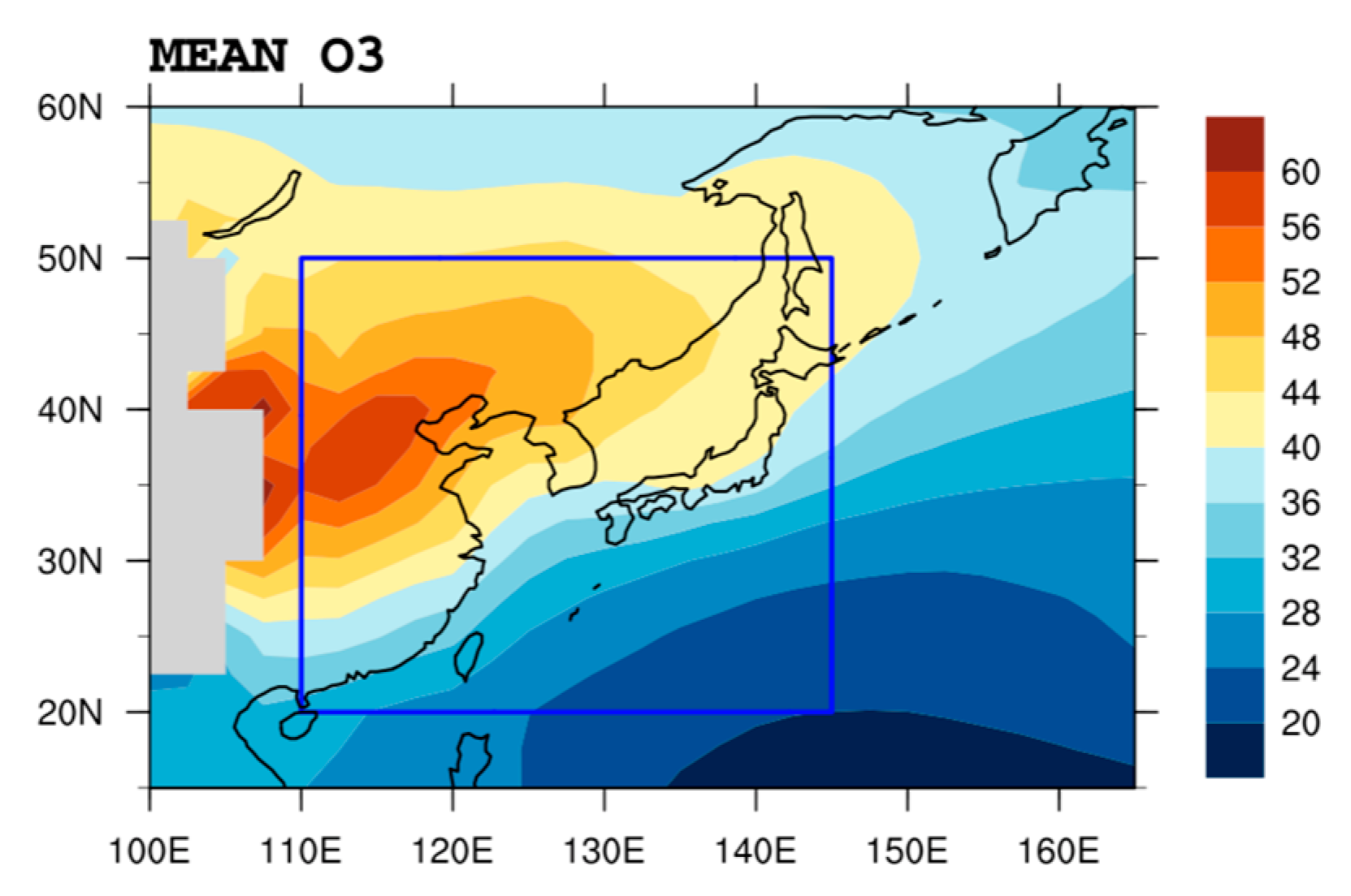
The vertical velocity (wa) was converted to omega (wap = −wa × × g, : air density, g: gravitational acceleration) [57], and the net ozone production rate was calculated as the difference between the rate of ozone production and the rate of ozone loss. The period analyzed is 1979–2010, and all variables were re-gridded to the same horizontal grid of 2.5° × 2.5° and 17 vertical layers before analysis. We used the multi-model mean (MMM) for each variable by averaging across models to improve the quality of calculations, since MMM tends to outperform individual models [58]. Figure 1 shows the MMM near-surface ozone during summer (June–July–August) with high concentration in East Asian continental region and low concentration in the equatorial western Pacific. The elevated ozone concentration in East Asia is attributed to increases in the anthropogenic emissions of precursors [23,59]. It is also noted that the low level of ozone in the equatorial western Pacific is caused by enhanced convection [60].
To focus on the interannual variability, MMM anomalies were calculated by removing the seasonal cycle. The empirical orthogonal function (EOF) analysis [61] was then applied to reveal the dominant spatiotemporal variability of summer ozone in the East Asian region (20° N–50° N and 110° E–145° E; see box in Figure 1). Notably, given any space-time fields (i.e., here, MMM ozone anomaly), EOF analysis captures a set of orthogonal spatial patterns along with those associated with principal components (PC time series). The linear regression analysis was also applied against the PC time series to access the relationship between the EOF modes of near-surface ozone and atmospheric fields.
3. Results and Discussion
3.1. Increasing Trend of Ozone Concentration During Summer in East Asia
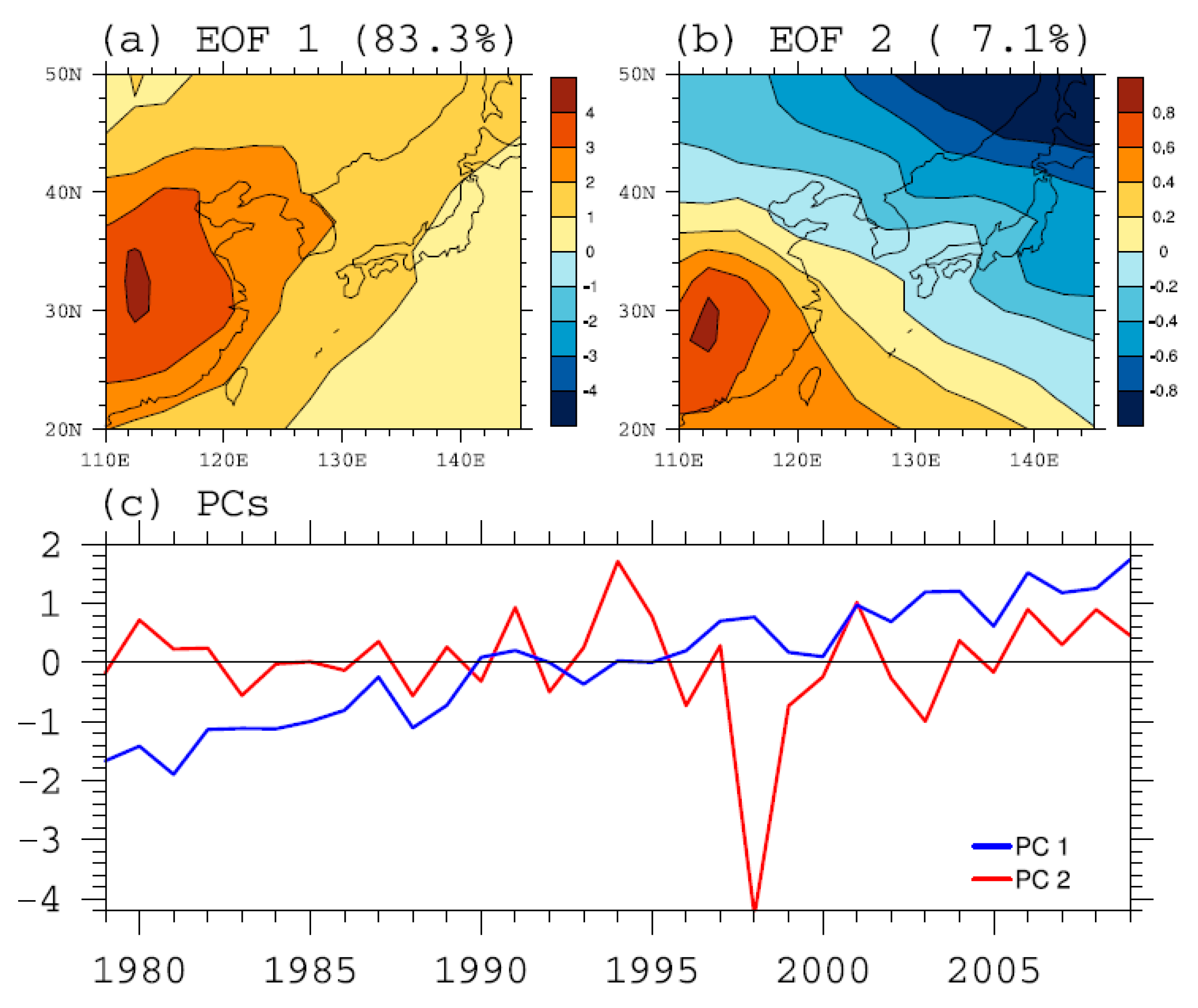
The results of the EOF analysis of the MMM ozone data for the East Asian region (20°N–50° N and 110°E–145° E) during the summer are shown in Figure 2, which depicts the two leading modes of the East Asian ozone at 850 hPa. The first mode (EOF1) shows a positive signal throughout East Asia centered in China, accounting for 83.3% of the total ozone variability (Figure 2a). By contrast, the second mode (EOF2) exhibits a dipole pattern with a positive ozone anomaly center in China and a negative northeastern region, which explains only 7.1% of the total variance (Figure 2b). The associated PC time series (PC1 and PC2, respectively) show a significant increasing trend with some interannual variability superimposed for EOF1, but prominent interannual variability for EOF2 (Figure 2c). This increasing trend in PC1, as mentioned above, clearly reflects the increase in the emission of ozone precursors over East Asia [23,59]. Meanwhile, the interannual variability of PCs implies that ozone variability might be influenced by the East Asian summer monsoon as well as ENSO [17,27], which we discuss in Section 3.2 and Section 3.3.
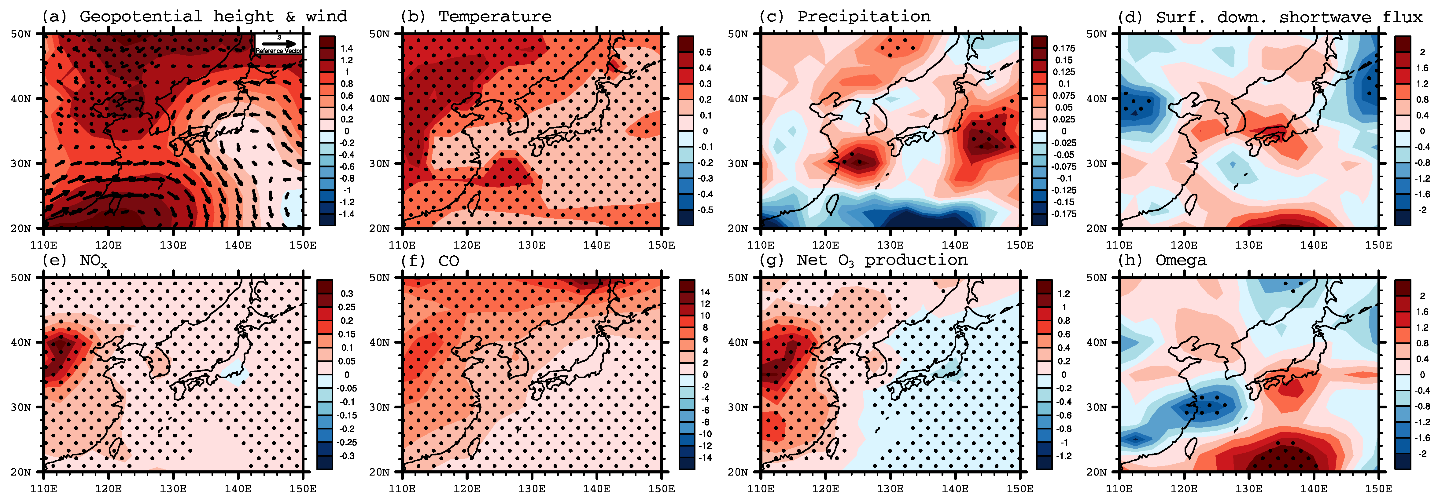
A regression analysis of the PC1 time series and atmospheric variables known to be related to ozone variation was performed to examine whether these features are present in the CCMI models. Figure 3 shows that the geopotential height, temperature, NOx, and CO concentration are all generally increasing in East Asia, indicating that the rising anthropogenic emission, more stable atmosphere, and warmer environment have contributed to the long-term increase in ozone concentration (Figure 2). The net ozone production (Figure 3g) is also increasing in China, as is the amount of ozone produced. Both ozone (Figure 2a) and ozone precursors (Figure 3e,f) are likely to be transported from the continental region to the Pacific Ocean via prevailing winds (Figure 3a), meaning that ozone can be a hemispheric pollutant [8]. Interestingly, precipitation, surface shortwave radiation, and omega have little correlation with the increase in ozone and rather localized structures (Figure 3c,d,h), suggesting that the changes in atmospheric circulation due to altered climate may have little influence on long-term ozone trends in East Asia if warming is not considered.
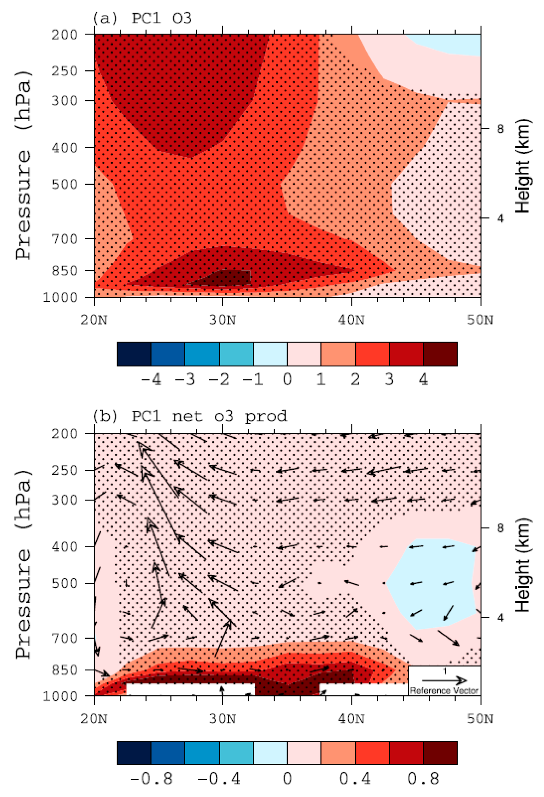
The vertical ozone, net ozone production, and circulation patterns were analyzed by calculating the average within an area between 110° E–120° E, where the concentration of ozone and ozone precursors was greatly increased (Figure 2a). As seen in Figure 4a, when an increase in the amount of ozone is seen in the lower troposphere, the ozone also increases in the upper troposphere. Note also that this vertical structure of tropospheric ozone increases is well consistent with northerly-upward motions (Figure 4b), thus bringing ozone-rich air from surface sources in China. These results indicate that the surface and upper atmosphere are closely connected not only dynamically but also chemically through human activities. It is also interesting to note that anthropogenically generated ozone acts as a greenhouse gas, which could impact the large-scale circulation [62]. Our results also imply that, in addition to local sources near the surface, the upward transport of ozone may be an important contributor to climate change, which needs further investigation.
3.2. Interannual Variability of Detrended Ozone During Summer in East Asia
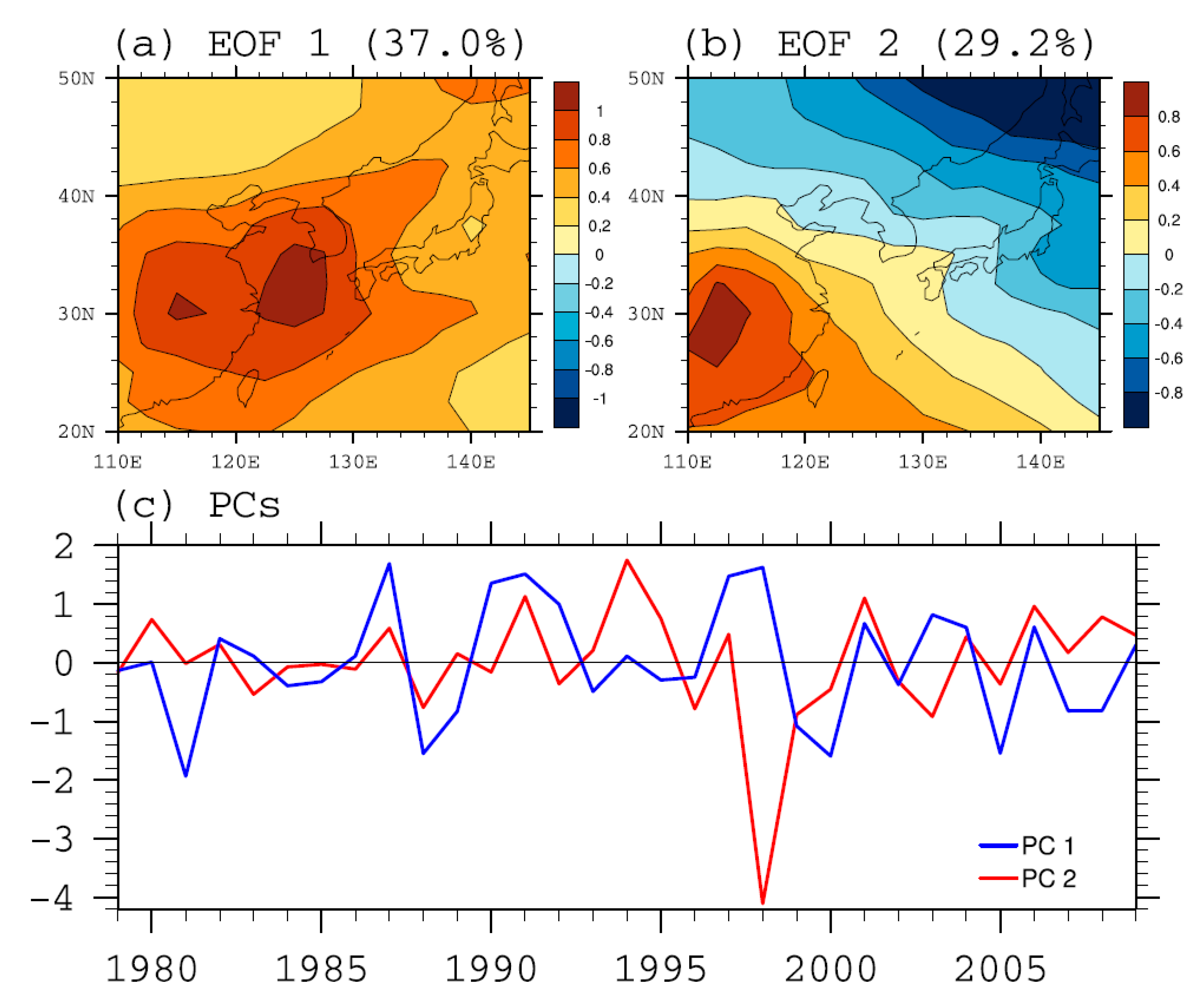
The increasing trend dominates the ozone variability over the East Asian region (Figure 2), which hampers the analysis of ozone levels at the interannual scale. This linear trend was therefore removed to further examine the interannual variability of ozone. Note that a similar procedure was then carried out as that described in Section 3.1 and shown in Figure 5. The first EOF mode of detrended ozone shows a positive ozone signal across East Asia, especially over eastern China and the Yellow Sea (Figure 5a). The PC1 time series is identical to the PC1 time series seen in Figure 2c (r = 0.98, p < 0.0001), if the trend is removed from the latter. This similarity indicates that the EOF analysis of detrended ozone can capture the interannual variability reasonably well, which is hidden in non-detrended ozone with a strong positive trend (blue line in Figure 2c). The spatial pattern and PC time series of the second mode of detrended ozone are nearly identical to those of the non-detrended second mode (Figure 2), except that the fraction of accounted for ozone variance increases to 22.1%.
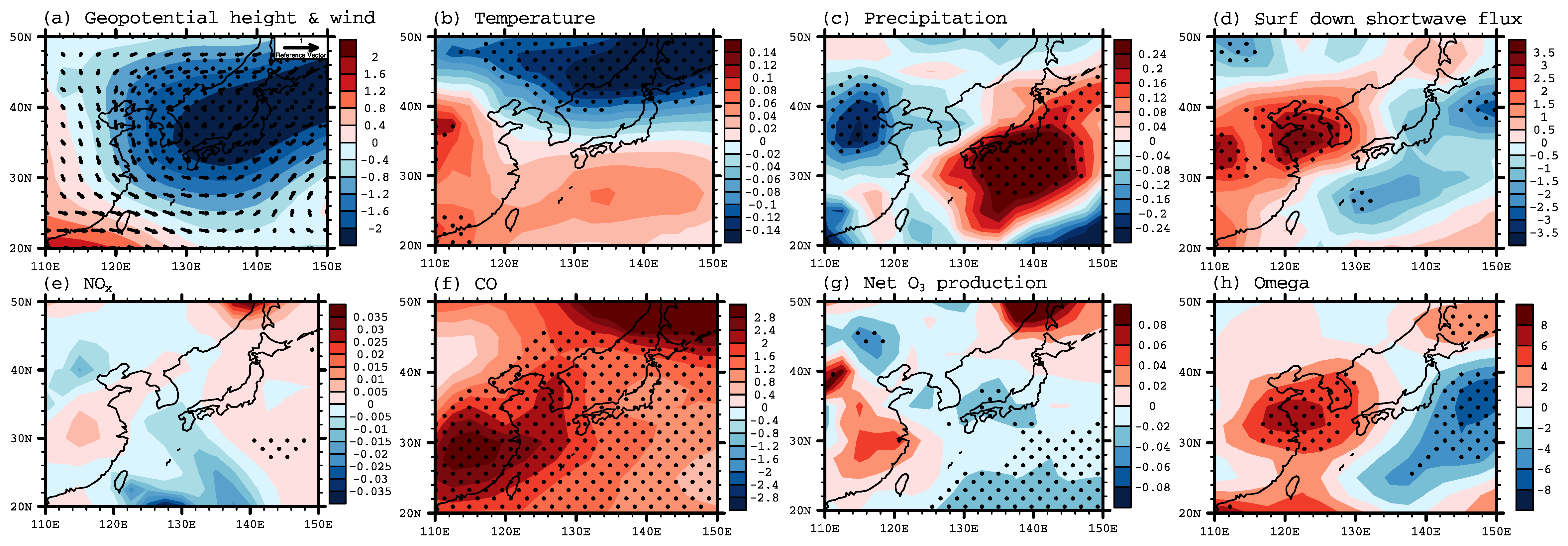
To understand the mechanism behind the ozone variability associated with the EOF1 of detrended ozone (Figure 5a), a regression analysis of atmospheric and chemical variables was performed against the PC1 (blue line in Figure 5c). Figure 6 shows that descending motions have appeared over China and Korea, and this is consistent with the reduced precipitation and increase in the surface downwelling solar radiation. Meanwhile, the low-pressure anomaly is located in northern Japan, accompanied by the northerly winds in the region 110° E–130° E. Note that NOx does not show any significant relationship with the ozone interannual variability of EOF1, whereas CO has a strong correlation. This interannual variability may influence the intercontinental transport of ozone from East Asia to western America [8]. Therefore, if the interannual variability is combined with the positive trend of ozone shown in Figure 2a, the East Asian region is expected to experience high concentrations of ozone, and in turn plays a more important role in the variation of hemispheric tropospheric ozone levels.
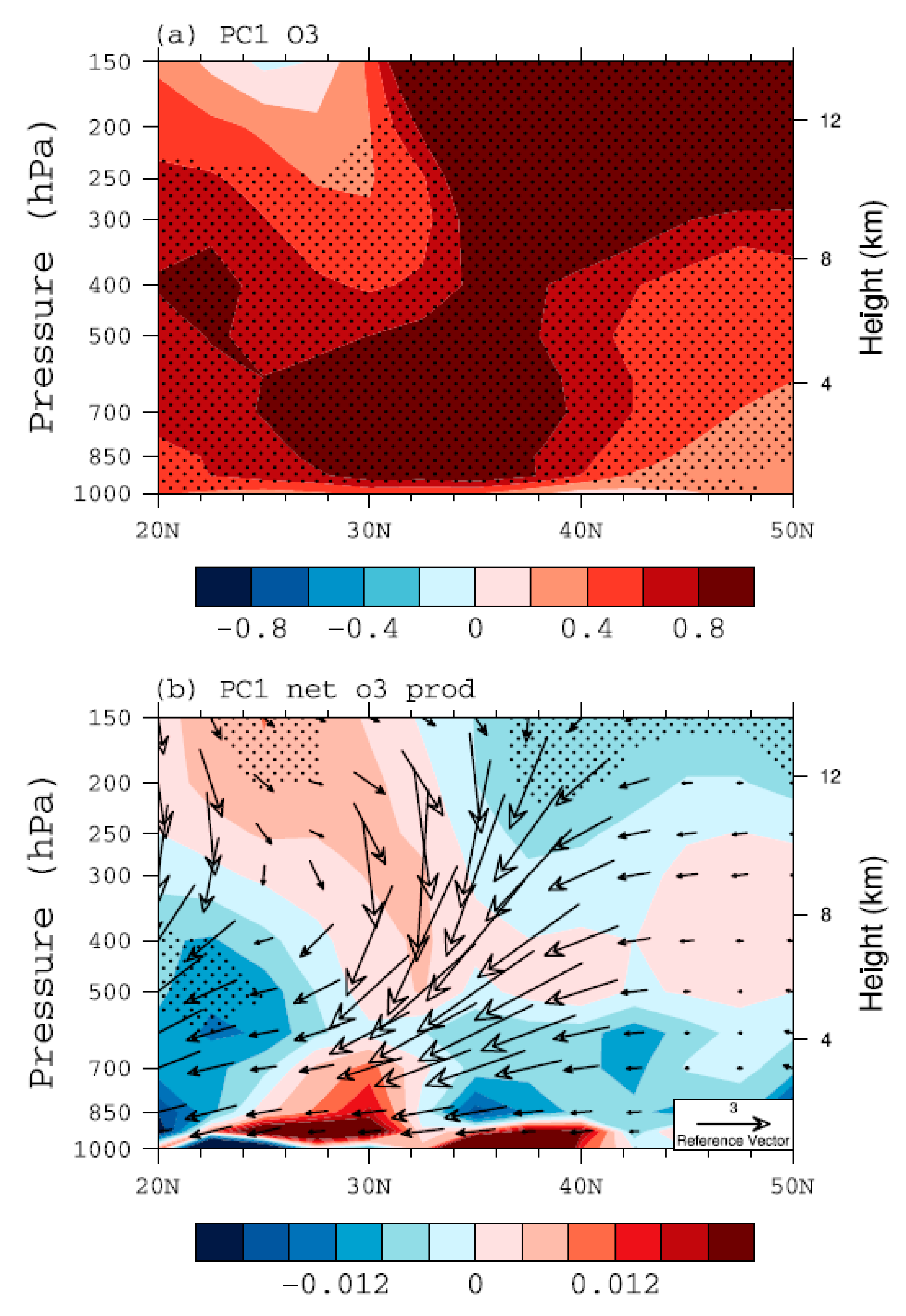
Figure 7 shows the regressed vertical ozone, circulations, and net ozone production over 120°–130° E against PC1 (blue line in Figure 5c), where a large positive ozone anomaly appeared as shown in Figure 5a. The concentration of ozone has increased over the entire troposphere, especially along with the northerly-downward air flows. Given the net ozone production is rather confined near the surface, this concurrent correlation indicates that the main reason for the increase in tropospheric ozone (Figure 6a) is the downward transport of ozone from the upper troposphere and possibly the stratosphere as well [5,63].
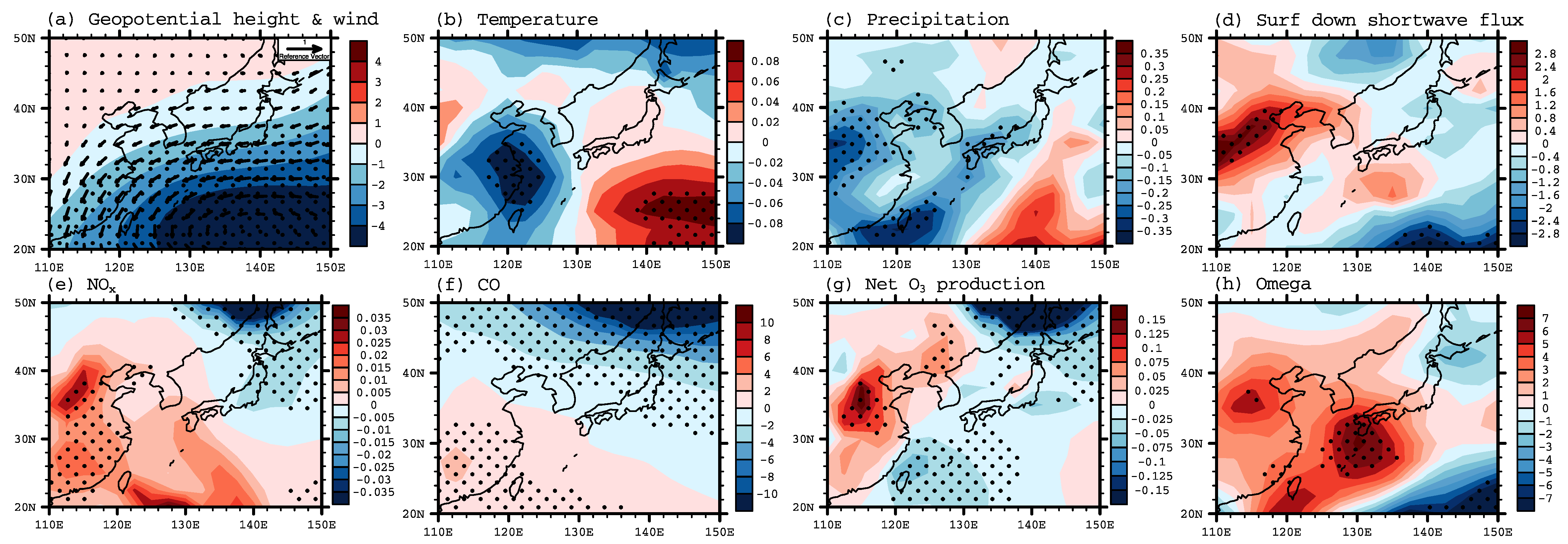
As mentioned above, the spatiotemporal patterns of the second mode are almost identical for non-detrended and detrended ozone (Figure 2 and Figure 5, respectively). Therefore, here, we focus on the second EOF mode of detrended ozone, as the following results are not sensitive to this choice. The regressed fields against the PC2 time series show that northeasterly winds are prevalent in China where the positive ozone anomaly is larger, together with significantly reduced precipitation and temperature (Figure 8). NOx and CO levels appear to increase. Note that 500 hPa omega exhibits descending motions, suggesting that ozone transported from the upper troposphere contributes to the increase in surface ozone.
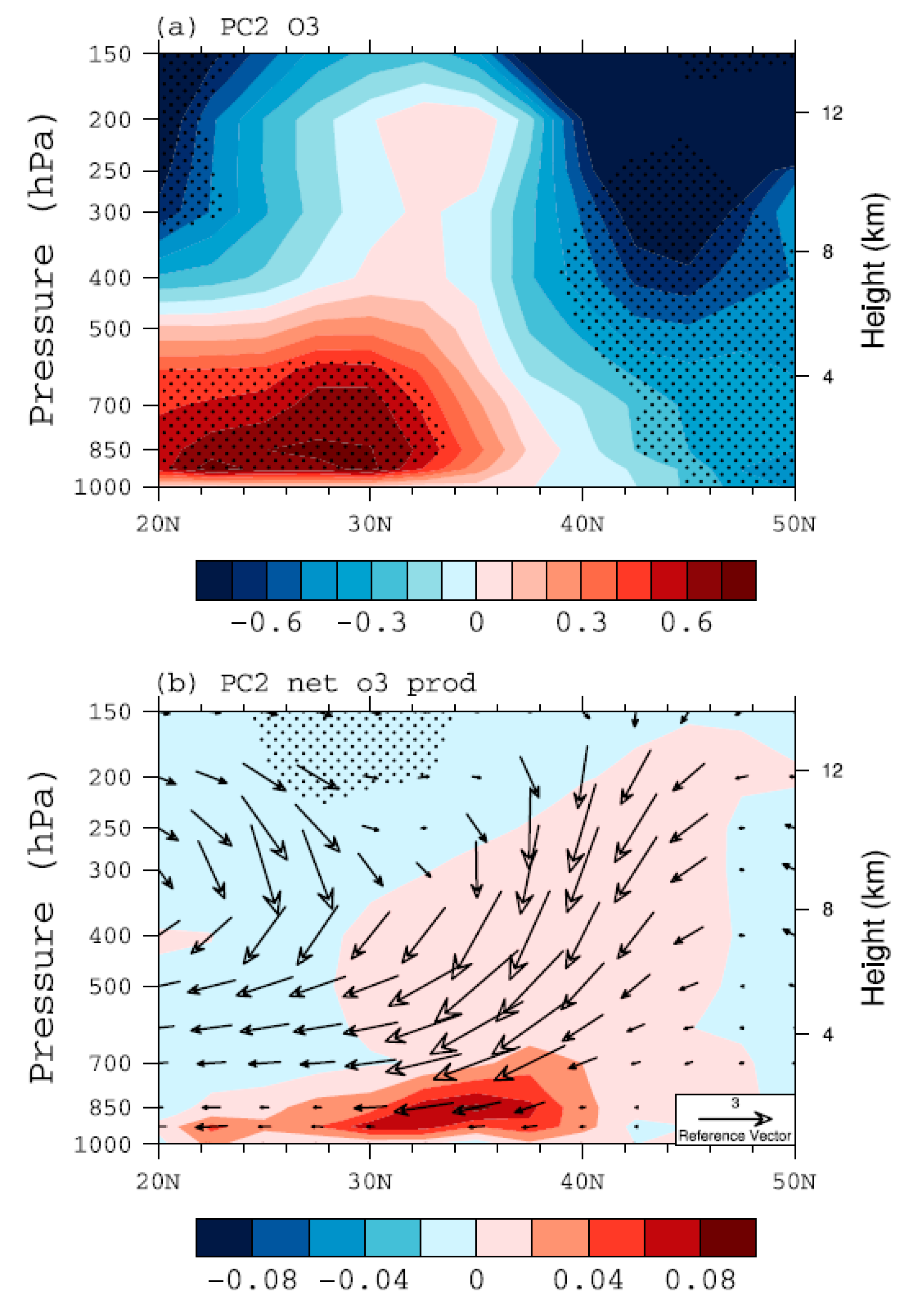
Figure 9 shows the results of regression analysis using PC2 on the average vertical ozone, net ozone production, and wind fields in the region between 110° E–120° E, where there is an obvious increase in ozone concentration. The increase in the ozone concentration of the lower troposphere continues up to a level of 500 hPa. Simultaneously, the descending motions start at a latitude of approximately 40° N in the upper troposphere and become northerly winds at the lower troposphere (>500 hPa), which eventually leads to an increase in ozone over China (Figure 5b) by the transport of high-ozone air mass. Here, it is interesting to note that there are some obvious differences between the two EOF modes, as indicated in Figure 7 and Figure 9. The near-surface ozone variability of the former can be more related to upper atmosphere, probably the net transport from the stratosphere. The vertically tilted pressure structure (Figure 6) also gives this possibility because stratosphere–troposphere exchange operates mainly on synoptic-scale eddies [64].
3.3. Ozone Variation, East Asia Summer Monsoon and ENSO
As shown in Figure 8, the second mode of near-surface ozone during the summer in East Asia is related to the decrease in precipitation and the increase in shortwave radiation, especially in the inland areas of China. These features can be associated with the weakening of the East Asian summer monsoon [17,65]. The factors that influence the behavior of the East Asian summer monsoon include the western Pacific subtropical high and ENSO [66]. For example, the movement of monsoonal rain bands is well correlated with the movement of the boundary of the western Pacific subtropical high [67]. The ENSO is known to affect the intensity of this western Pacific subtropical high and then influence the summer monsoon in East Asia.
Therefore, it is reasonable to anticipate that ENSO and western Pacific subtropical high may influence the ozone distribution of EOF2. This is confirmed by the correlation coefficients between PC time series and various indices (Table 2). Here, the western Pacific subtropical high index (WPSHI) is defined as the normalized summer 850 hPa geopotential height anomalies averaged over the region (115° E–150° E, 15° N–25° N) [68]. Interestingly, PC2 shows very strong negative correlations with the preceding NINO3 indices (DJF and MAM) and WPSHI, whereas PC1 does not show any correlation with WPSH. Considering the cyclonic circulation over the western Pacific (Figure 8a) comes with negative WPSHI, these negative correlations result mainly from the weakened western Pacific subtropical high during summer after the occurrence of La Niña during the previous winter.
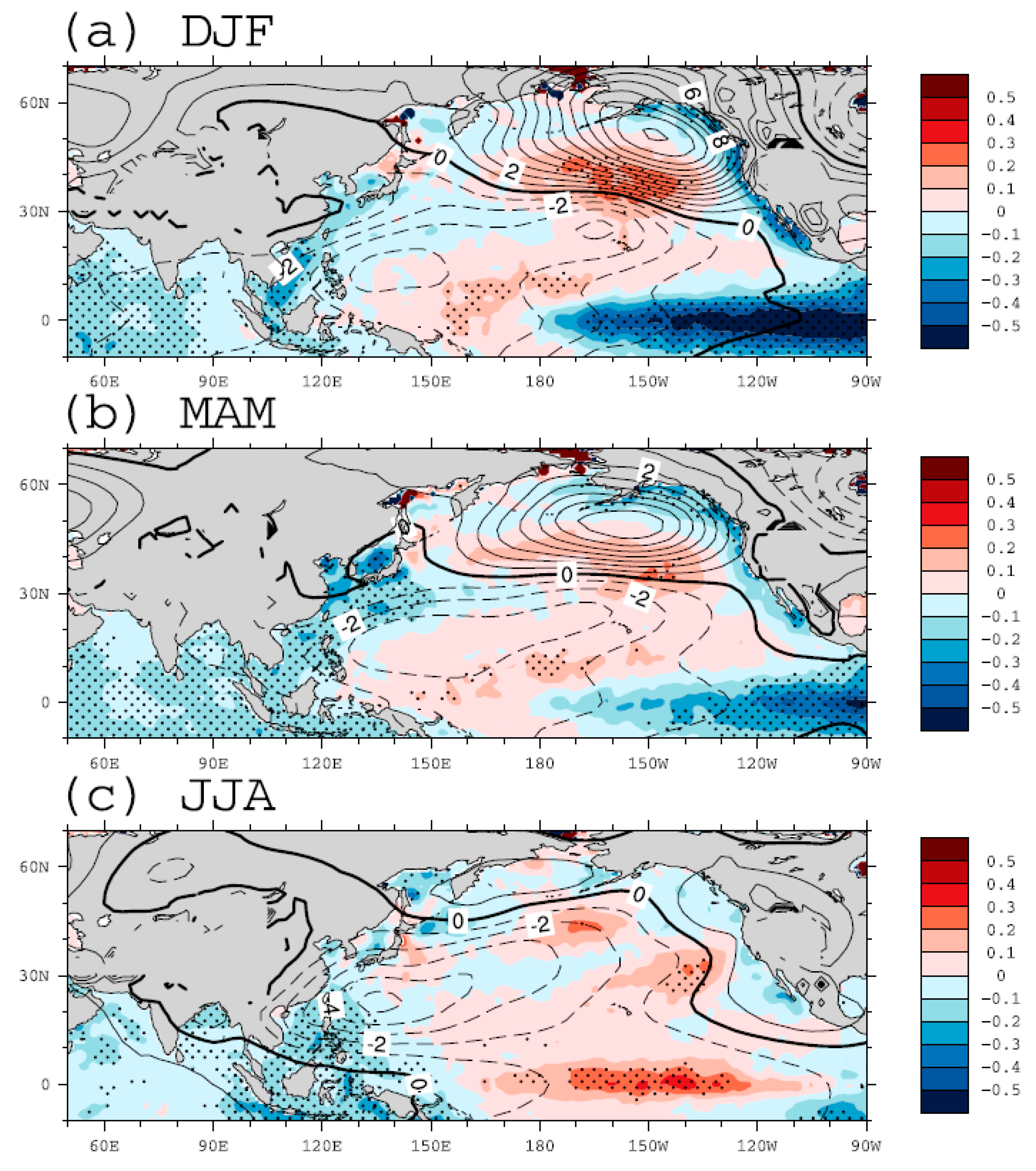
Evidently, this lagged relationship between the EOF2 of ozone, western Pacific subtropical high and ENSO can be seen in Figure 10. The negative sea surface temperature (SST) anomaly appeared in the equatorial eastern Pacific during the previous winter (DJF), indicating the presence of La Niña. This negative anomaly became diminished in the spring (MAM), and during the summer, positive anomalies appeared along the equatorial central Pacific, indicating the development of El Niño. Simultaneously, in the subtropical region of the western Pacific, a negative geopotential height anomaly was apparent during the winter, and the negative anomalies became stronger in the spring and summer, as consistent with previous studies [66,69,70]. These studies suggested that the anomalous western Pacific subtropical high plays a crucial role in linking ENSO and the East Asian summer monsoon. Here, we argue that ENSO can influence not only climate but also ozone levels in East Asia through the western Pacific subtropical high.
To better understand the role of the western Pacific subtropical high in modulating the ozone anomalies in East Asian region, we analyzed correlation coefficients between PC2 time series, DJF NINO3 and JJA WPSH indices for each model (Table 3). Note that HadISST data were used for the CCMI models simulations; each model has the same DJF NINO3 index. Similarly, we used a multi-model averaged WPSH index, because each model has a different performance when simulating the western Pacific subtropical high. Six models out of the 12 showed significant correlations both for DJF NINO3 and JJA WPSH indices, as indicated in bold in Table 3.
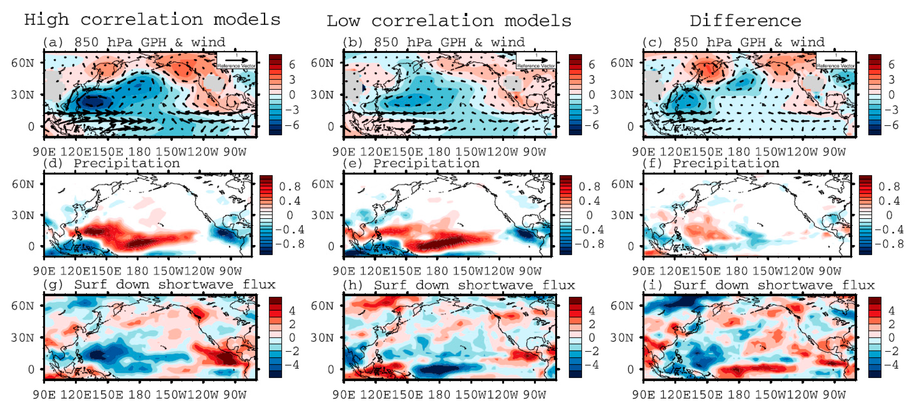
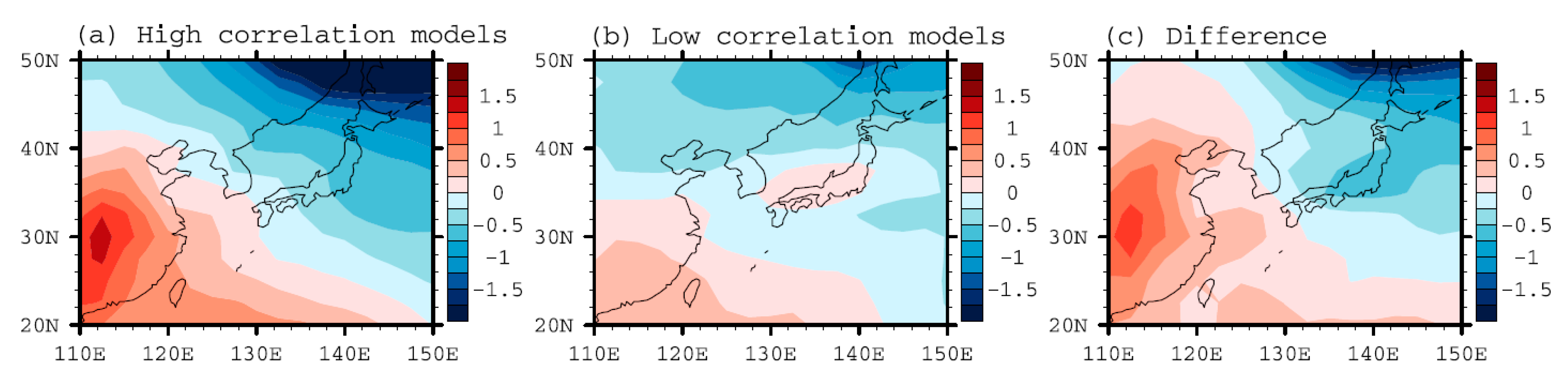
Based on this result, the models were categorized into those with high correlation (GRIMS-CCM, MRI-ESM1r1, NIWA-UKCA, MOCAGE, EMAC-L90MA, and CCSRNIES-MIROC3.2) and low correlation (CMAM, SOCOL3, GEOSCCM, UMUKCA-UCAM, ULAQ-CCM, and EMAC-L47MA). Using the PC2 time series of Figure 5, regression analysis was performed on the ensemble-averaged geopotential height, wind fields, precipitation, and the shortwave radiation reaching the surface in each group (Figure 11). Models with high correlation coefficients were found to clearly simulate the weakening of the western Pacific subtropical high when compared to models with low correlation coefficients. A reason for the different behavior of western Pacific subtropical high can be found with the precipitation difference (Figure 11f), exhibiting a positive precipitation anomaly over the western North Pacific (centered at 140° E, 20° N), which in turn intensified convection activities. It was also simulated that the amount of solar radiation reaching the surface increased in China (Figure 11i), causing an increase in the net photochemical production of near-surface ozone (Figure 9b) and leading to an increase in near-surface ozone (Figure 12). These results suggest that the cyclonic circulation anomaly associated with the weakened western Pacific subtropical high is key to understanding how ENSO affects the East Asian ozone. In the low-correlation models, ozone concentration does not increase substantially in China (Figure 12b). This lack of ozone increase can be attributed to reduced solar radiation (Figure 11h).
4. Conclusions
This study analyzed the 12 models’ results from the CCMI project to identify the leading EOF modes of near-surface (850 hPa) ozone during the summer season over East Asia and to investigate the associated ozone precursors as well as atmospheric conditions based on linear regression analysis. Using the non-detrended ozone concentrations, it was found that the prominent change in ozone over the East Asian region was the increasing trend of ozone concentration (Figure 2a), which could be related to the increase in anthropogenic ozone precursor emissions in China (Figure 3). Both ozone and its precursors have spread from the area in which they are generated, eventually influencing the whole of East Asia.
We also used the detrended ozone to focus on interannual variability and revealed that the first two leading modes of ozone are closely linked to meteorological conditions. The EOF1 exhibits a monopole of ozone variation centered at China and the Korean Peninsula (Figure 5a). We find this EOF1 pattern is associated with synoptic scale disturbances, accompanied by downward motion as well as enhanced solar radiation on the west side of mid-latitude cyclones (i.e., after the cold front has passed) (Figure 6). While the positive net ozone production is strongly concentrated near the surface, the ozone exhibits overall increases in the entire troposphere (Figure 7), thus indicating the influence of stratosphere–troposphere exchange, which needs more detailed analysis. In addition, the northeasterly wind that blows along the coastline might lead to both ozone and ozone precursors becoming trapped in the inland areas of eastern China, causing excessive ozone levels.
The EOF2 shows a dipole ozone anomaly between China and northeastern Asia (Figure 5b). The corresponding PC2 time series is significantly correlated with the western Pacific subtropical high and ENSO. Regression analysis reveals that circulation changes associated with the western Pacific subtropical high after the peak of La Niña in the previous winter are the most prominent source of interannual near-surface ozone variability during the summer in East Asia. When the western Pacific subtropical high is weak, a strong north-easterly flow occurs along China, the Korean Peninsula, and Japan, thus reducing the summer monsoon rainfall and leading to more insolation near the surface. Note that the weakening of the western Pacific subtropical high during summer after La Niña can be understood as the Pacific–East Asian teleconnection [66,69]. These meteorological changes result in excessive ozone concentration in China due to both the advection of ozone-rich air and stronger photochemical production (Figure 9). Note that this interannual variation of ozone works in combination with the long-term increasing trend, which could further add to the concentration of ozone seen in East Asia. Based on the correlation coefficients between PC2 time series, NINO3 and WPSH indices, CCMI models can be classified into two groups: those six models with good relationships between indices, and the six models with insignificant relationships. The results also suggest that the concurrent changes including the weakening of the western Pacific subtropical high and decaying of La Niña can enhance ozone concentration in China.
Our results are obtained from chemistry–climate models that consider the interaction between atmospheric chemicals and the climate. It is therefore necessary to perform a similar analysis using in situ observations and remote sensing data. Finally, we note that, if the anthropogenic emission of ozone precursors decreases, the second EOF mode of ozone concentrations will become more important in a future warmer world, since ENSO will be more active [71]. It is therefore necessary to understand how the linkage between East Asian ozone and ENSO may vary as global warming is intensified, which needs further study.
Author Contributions
Conceptualization, B.-K.M. and J.W.; writing—original draft preparation, J.W.; Data curation, H.-J.P. and H.L.; writing-review and editing, J.W., H.-J.P., H.L., and B.-K.M. All authors have read and agreed to the published version of the manuscript.
Funding
This work was supported by the National Research Foundation of Korea (NRF) grant funded by the Korean government (MSIT) (No. 2019R1A2C1008549).
Acknowledgments
We acknowledge the modeling groups for making their simulations available for this analysis, the joint WCRP SPARC/IGAC Chemistry–Climate Model Initiative (CCMI) for organizing and coordinating the model simulations and data analysis activity, and the British Atmospheric Data Centre (BADC) for collecting and archiving the CCMI model output. The authors are grateful to the international modeling groups of National Institute for Environmental Studies (NIES) in Japan, Canadian Centre for Climate Modelling and Analysis (CCCma), Environment and Climate Change Canada in Canada, Modular Earth Submodel System (Messy)-Consortium in Germany, National Aeronautics and Space Administration’s Goddard Space Flight Center (NASA/GSFC) in United States of America, School of Earth and Environmental Sciences, Seoul National University in Korea, Meteo-France, Centre National de la Recherche Scientifique (CNRS) in France, Meteorological Research Institute (MRI) in Japan, National Institute of Water and Atmospheric Research (NIWA) in New Zealand, Physical Meteorological Observatory in Davos and World Radiation Center (PMOD/WRC) and Institute for Atmospheric and Climate Science in ETH Zurich (IAC/ETHZ) in Switzerland, University of L’Aquila in Italy, and University of Cambridge in United Kingdom for providing their model data for this study.
Conflicts of Interest
The authors declare no conflict of interest.
References
- Anenberg, S.C.; Schwartz, J.; Shindell, D.; Amann, M.; Faluvegi, G.; Klimont, Z.; Janssens-Maenhout, G.; Pozzoli, L.; Dingenen, R.V.; Vignati, E.; et al. Global air quality and health co-benefits of mitigating near-term climate change through methane and black carbon emission controls. Environ. Health Perspect. 2016, 120, 831–839. [Google Scholar] [CrossRef] [Green Version]
- Akimoto, H.; Kurokawa, J.; Sudo, K.; Nagashima, T.; Takemura, T.; Klimont, Z.; Amann, M.; Suzuki, K. SLCP co-control approach in East Asia: Tropospheric ozone reduction strategy by simultaneous reduction of NOx/NMVOC and methane. Atmos. Environ. 2016, 122, 588–595. [Google Scholar] [CrossRef]
- Scovronick, N.; Dora, C.; Fletcher, E.; Haines, A.; Shindell, D. Reduce short-lived climate pollutants for multiple benefits. Lancet 2015, 386, e28–e31. [Google Scholar] [CrossRef]
- Hegglin, M.I.; Shepherd, T.G. Large climate-induced changes in ultraviolet index and stratosphere-to-troposphere ozone flux. Nat. Geosci. 2009, 2, 687–691. [Google Scholar] [CrossRef]
- Lelieveld, J.; Dentener, F.J. What controls tropospheric ozone? J. Geophys. Res. 2000, 205, 3531–3551. [Google Scholar] [CrossRef]
- Neu, J.L.; Flury, T.; Manney, G.L.; Santee, M.L.; Livesey, N.J.; Worden, J. Tropospheric ozone variations governed by changes in stratospheric circulation. Nat. Geosci. 2014, 7, 340–344. [Google Scholar] [CrossRef]
- Fishman, J.; Ramanathan, V.; Crutzen, P.J.; Liu, S.C. Tropospheric Ozone and Climate. Nature 1979, 282, 818–820. [Google Scholar] [CrossRef]
- Verstraeten, W.W.; Neu, J.L.; Williams, J.E.; Bowman, K.W.; Worden, J.R.; Boersma, K.F. Rapid increases in tropospheric ozone production and export from China. Nat. Geosci. 2015, 8, 690–695. [Google Scholar] [CrossRef]
- Kurokawa, J.; Ohara, T.; Uno, I.; Hayasaki, M.; Tanimoto, H. Influence of meteorological variability on interannual variations of springtime boundary layer ozone over Japan during 1981–2005. Atmos. Chem. Phys. 2009, 9, 6287–6304. [Google Scholar] [CrossRef] [Green Version]
- Lin, M.; Holloway, T.; Oki, T.; Streets, D.G.; Richter, A. Multi-scale model analysis of boundary layer ozone over East Asia. Atmos. Chem. Phys. 2009, 9, 3277–3301. [Google Scholar] [CrossRef] [Green Version]
- Yang, Y.; Liao, H.; Li, J. Impacts of the East Asian summer monsoon on interannual variations of summertime surface-layer ozone concentrations over china. Atmos. Chem. Phys. 2014, 14, 6867–6879. [Google Scholar] [CrossRef] [Green Version]
- Stathopoulou, E.; Mihalakakou, G.; Santamouris, M.; Bagiorgas, H.S. On the impact of temperature on tropospheric ozone concentration levels in urban environments. J. Earth Syst. Sci. 2008, 117, 227–236. [Google Scholar] [CrossRef]
- Walcek, C.J.; Yuan, H.H. Calculated influence of temperature-related factors on ozone formation rates in the lower troposphere. J. Appl. Meteorol. 1995, 34, 1056–1069. [Google Scholar] [CrossRef] [Green Version]
- Fusco, A.C.; Logan, J.A. Analysis of 1970–1995 trends in tropospheric ozone at Northern Hemisphere midlatitudes with the geos-chem model. J. Geophys. Res. Atmos. 2003, 108, 4449. [Google Scholar] [CrossRef]
- Knowland, K.E.; Doherty, R.M.; Hodges, K.I.; Ott, L.E. The influence of mid-latitude cyclones on European background surface ozone. Atmos. Chem. Phys. 2017, 17, 12421–12447. [Google Scholar] [CrossRef] [Green Version]
- Roelofs, G.J.; Kentarchos, A.S.; Trickl, T.; Stohl, A.; Collins, W.J.; Crowther, R.A.; Hauglustaine, D.; Klonecki, A.; Law, K.S.; Lawrence, M.G.; et al. Intercomparison of tropospheric ozone models: Ozone transport in a complex tropopause folding event. J. Geophys. Res. 2003, 108, 8529. [Google Scholar] [CrossRef] [Green Version]
- Wie, J.; Moon, B.K. Impact of the western north Pacific subtropical high on summer surface ozone in the Korean peninsula. Atmos. Pollut. Res. 2018, 9, 655–661. [Google Scholar] [CrossRef]
- Park, H.J.; Moon, B.K.; Wie, J. Characteristics of summer tropospheric ozone over East Asia in a chemistry-climate model simulation. J. Korean Earth Sci. Soc. 2017, 38, 345–356. [Google Scholar] [CrossRef]
- Chandra, S.; Ziemke, J.R.; Min, W.; Read, W.G. Effects of 1997–1998 El Niño on tropospheric ozone and water vapor. Geophys. Res. Lett. 1998, 25, 3867–3870. [Google Scholar] [CrossRef] [Green Version]
- Sudo, K.; Takahashi, M. Simulation of tropospheric ozone changes during 1997–1998 El Niño: Meteorological impact on tropospheric photochemistry. Geophys. Res. Lett. 2001, 28, 4091–4094. [Google Scholar] [CrossRef]
- Ziemke, J.R.; Chandra, S. La Niña and El Niño-induced variabilities of ozone in the tropical lower atmosphere during 1970–2001. Geophys. Res. Lett. 2003, 30, 1142. [Google Scholar] [CrossRef]
- Granier, C.; Bessagnet, B.; Bond, T.; D’Angiola, A.; van der Gon, H.D.; Frost, G.J.; Heil, A.; Kaiser, J.W.; Kinne, S.; Klimont, Z.; et al. Evolution of anthropogenic and biomass burning emissions of air pollutants at global and regional scales during the 1980–2010 period. Clim. Chang. 2011, 109, 163–190. [Google Scholar] [CrossRef]
- Van Der A, R.J.; Eskes, H.J.; Boersma, K.F.; Van Noije, T.P.C.; Van Roozendael, M.; De Smedt, I.; Peters, D.H.M.U.; Meijer, E.W. Trends, seasonal variability and dominant NOx source derived from a ten year record of NO2 measured from space. J. Geophys. Res. Atmos. 2008, 113, D04302. [Google Scholar] [CrossRef]
- Lee, S.S.; Seo, Y.W.; Ha, K.J.; Jhun, J.G. Impact of the western north Pacific subtropical high on the East Asian monsoon precipitation and the Indian ocean precipitation in the boreal summertime. Asia Pac. J. Atmos. Sci. 2013, 49, 171–182. [Google Scholar] [CrossRef]
- Kley, D.; Crutzen, P.J.; Smit, H.G.J.; Vomel, H.; Oltmans, S.J.; Grassl, H.; Ramanathan, V. Observations of near-zero ozone concentrations over the convective pacific: Effects on air chemistry. Science 1996, 274, 230–233. [Google Scholar] [CrossRef]
- He, Y.J.; Uno, I.; Wang, Z.F.; Pochanart, P.; Li, J.; Akimoto, H. Significant impact of the East Asia monsoon on ozone seasonal behavior in the boundary layer of eastern china and the west Pacific region. Atmos. Chem. Phys. 2008, 8, 7543–7555. [Google Scholar] [CrossRef] [Green Version]
- Wie, J.; Moon, B.K. Seasonal relationship between meteorological conditions and surface ozone in Korea based on an offline chemistry-climate model. Atmos. Pollut. Res. 2016, 7, 385–392. [Google Scholar] [CrossRef]
- Eyring, V.; Lamarque, J.F.; Hess, P.; Arfeuille, F.; Bowman, K.; Chipperfiel, M.P.; Duncan, B.; Fiore, A.; Gettelman, A.; Giorgetta, M.A.; et al. Overview of IGAC/SPARC chemistry-climate model initiative (CCMI) community simulations in support of upcoming ozone and climate assessments. SPARC Newsl. 2013, 40, 48–66. [Google Scholar]
- Son, S.W.; Han, B.R.; Garfinkel, C.I.; Kim, S.Y.; Park, R.; Abraham, N.L.; Akiyoshi, H.; Archibald, A.T.; Butchart, N.; Chipperfield, M.P.; et al. Tropospheric jet response to Antarctic ozone depletion: An update with Chemistry-Climate Model Initiative (CCMI) models. Environ. Res. Lett. 2018, 13, 054024. [Google Scholar] [CrossRef]
- Orbe, C.; Yang, H.; Waugh, D.W.; Zeng, G.; Morgenstern, O.; Kinnison, D.E.; Lamarque, J.F.; Tilmes, S.; Plummer, D.A.; Scinocca, J.F.; et al. Large-scale tropospheric transport in the Chemistry-Climate Model Initiative (CCMI) simulations. Atmos. Chem. Phys. 2018, 18, 7217–7235. [Google Scholar] [CrossRef] [Green Version]
- Hegglin, M.I.; Lamarque, J.-F. The IGAC/SPARC Chemistry-Climate Model Initiative Phase-1 (CCMI-1) Model Data Output, NCAS British Atmospheric Data Centre. 20 February 2017. Available online: http://catalogue.ceda.ac.uk/uuid/9cc6b94df0f4469d8066d69b5df879d5 (accessed on 11 April 2018).
- Morgenstern, O.; Hegglin, M.I.; Rozanov, E.; O’Connor, F.M.; Abraham, N.L.; Akiyoshi, H.; Archibald, A.; Bekki, S.; Butchart, N.; Chipperfield, M.P.; et al. Review of the global models used within phase 1 of the Chemistry-Climate Model Initiative (CCMI). Geosci. Model Dev. 2017, 10, 639–671. [Google Scholar] [CrossRef] [Green Version]
- Lamarque, J.F.; Bond, T.C.; Eyring, V.; Granier, C.; Heil, A.; Klimont, Z.; Lee, D.; Liousse, C.; Mieville, A.; Owen, B.; et al. Historical (1850–2000) gridded anthropogenic and biomass burning emissions of reactive gases and aerosols: Methodology and application. Atmos. Chem. Phys. 2010, 10, 7017–7039. [Google Scholar] [CrossRef] [Green Version]
- Imai, K.; Manago, N.; Mitsuda, C.; Naito, Y.; Nishimoto, E.; Sakazaki, T.; Fujiwara, M.; Froidevaux, L.; von Clarmann, T.; Stiller, G.P.; et al. Validation of ozone data from the Superconducting Submillimeter-Wave Limb-Emission Sounder (SMILES). J. Geophys. Res. Atmos. 2013, 118, 5750–5769. [Google Scholar] [CrossRef] [Green Version]
- Akiyoshi, H.; Nakamura, T.; Miyasaka, T.; Shiotani, M.; Suzuki, M. A nudged chemistry-climate model simulation of chemical constituent distribution at northern high-latitude stratosphere observed by SMILES and MLS during the 2009/2010 stratospheric sudden warming. J. Geophys. Res. 2016, 121, 1361–1380. [Google Scholar] [CrossRef] [Green Version]
- Jonsson, A.I.; de Grandpré, J.; Fomichev, V.I.; McConnell, J.C.; Beagley, S.R. Doubled CO2-induced cooling in the middle atmosphere: Photochemical analysis of the ozone radiative feedback. J. Geophys. Res. 2004, 109, D24103. [Google Scholar] [CrossRef]
- Scinocca, J.F.; McFarlane, N.A.; Lazare, M.; Li, J.; Plummer, D. Technical Note: The CCCma third generation AGCM and its extension into the middle atmosphere. Atmos. Chem. Phys. 2008, 8, 7055–7074. [Google Scholar] [CrossRef] [Green Version]
- Jöckel, P.; Kerkweg, A.; Pozzer, A.; Sander, R.; Tost, H.; Riede, H.; Baumgaertner, A.; Gromov, S.; Kern, B. Development cycle 2 of the Modular Earth Submodel System (MESSy2). Geosci. Model Dev. 2010, 3, 717–752. [Google Scholar] [CrossRef] [Green Version]
- Jöckel, P.; Tost, H.; Pozzer, A.; Kunze, M.; Kirner, O.; Brenninkmeijer, C.A.M.; Brinkop, S.; Cai, D.S.; Dyroff, C.; Eckstein, J.; et al. Earth System Chemistry integrated Modelling (ESCiMo) with the Modular Earth Submodel System (MESSy) version 2.51. Geosci. Model Dev. 2016, 9, 1153–1200. [Google Scholar] [CrossRef] [Green Version]
- Molod, A.; Takacs, L.; Suarez, M.; Bacmeister, J.; Song, I.-S.; Eichmann, A. The GEOS-5 Atmospheric General Circulation Model: Mean Climate and Development from MERRA to Fortuna. NASA Tech. Rep. Ser. Glob. Modeling Data Assim. 2012, 28, 117. [Google Scholar]
- Molod, A.; Takacs, L.; Suarez, M.; Bacmeister, J. Development of the GEOS-5 atmospheric general circulation model: Evolution from MERRA to MERRA2. Geosci. Model Dev. 2015, 8, 1339–1356. [Google Scholar] [CrossRef] [Green Version]
- Oman, L.D.; Ziemke, J.R.; Douglass, A.R.; Waugh, D.W.; Lang, C.; Rodriguez, J.M.; Nielsen, J.E. The response of tropical tropospheric ozone to ENSO. Geophys. Res. Lett. 2011, 38, L13706. [Google Scholar] [CrossRef] [Green Version]
- Oman, L.D.; Douglass, A.R.; Ziemke, J.R.; Rodriguez, J.M.; Waugh, D.W.; Nielsen, J.E. The ozone response to ENSO in Aura satellite measurements and a chemistry-climate simulation. J. Geophys. Res. 2013, 118, 965–976. [Google Scholar] [CrossRef] [Green Version]
- Jeong, Y.-C.; Yeh, S.-W.; Lee, S.; Park, R.J. A global/regional integrated model system-chemistry climate model: 1. simulation characteristics. Earth Space Sci. 2019, 6, 2016–2030. [Google Scholar] [CrossRef]
- Josse, B.; Simon, P.; Peuch, V.-H. Radon global simulations with the multiscale chemistry and transport model MOCAGE. Tellus B 2004, 56, 339–3564. [Google Scholar] [CrossRef]
- Guth, J.; Josse, B.; Marécal, V.; Joly, M.; Hamer, P. First implementation of secondary inorganic aerosols in the MOCAGE version R2.15.0 chemistry transport model. Geosci. Model Dev. 2016, 9, 137–160. [Google Scholar] [CrossRef] [Green Version]
- Yukimoto, S.; Yoshimura, H.; Hosaka, M.; Sakami, T.; Tsujino, H.; Hirabara, M.; Tanaka, T.Y.; Deushi, M.; Obata, A.; Nakano, H.; et al. Meteorological Research Institute Earth System Model Version 1 (MRIESM1)—Model Description. Tech. Rep. MRI 2011, 64, 83. [Google Scholar]
- Yukimoto, S.; Adachi, Y.; Hosaka, M.; Sakami, T.; Yoshimura, H.; Hirabara, M.; Tanaka, T.Y.; Shindo, E.; Tsujino, H.; Deushi, M.; et al. A new global climate model of the Meteorological Research Institute: MRI-CGCM3—Model description and basic performance. J. Meteorol. Soc. Jpn. 2012, 90, 23–64. [Google Scholar] [CrossRef] [Green Version]
- Deushi, M.; Shibata, K. Development of a Meteorological Research Institute chemistry-climate model version 2 for the study of tropospheric and stratospheric chemistry. Pap. Meteorol. Geophys. 2011, 62, 1–46. [Google Scholar] [CrossRef] [Green Version]
- Stone, K.A.; Morgenstern, O.; Karoly, D.J.; Klekociuk, A.R.; French, W.J.; Abraham, N.L.; Schofield, R. Evaluation of the ACCESS—chemistry-climate model for the Southern Hemisphere. Atmos. Chem. Phys. 2016, 16, 2401–2415. [Google Scholar] [CrossRef] [Green Version]
- Morgenstern, O.; Braesicke, P.; O’Connor, F.M.; Bushell, A.C.; Johnson, C.E.; Osprey, S.M.; Pyle, J.A. Evaluation of the new UKCA climate-composition model—Part 1: The stratosphere. Geosci. Model Dev. 2009, 2, 43–57. [Google Scholar] [CrossRef] [Green Version]
- Morgenstern, O.; Zeng, G.; Abraham, N.L.; Telford, P.J.; Braesicke, P.; Pyle, J.A.; Hardiman, S.C.; O’Connor, F.M.; Johnson, C.E. Impacts of climate change, ozone recovery, and increasing methane on surface ozone and the tropospheric oxidizing capacity. J. Geophys. Res. Atmos. 2013, 118, 1028–1041. [Google Scholar] [CrossRef]
- Revell, L.E.; Tummon, F.; Stenke, A.; Sukhodolov, T.; Coulon, A.; Rozanov, E.; Garny, H.; Grewe, V.; Peter, T. Drivers of the tropospheric ozone budget throughout the 21st century under the medium-high climate scenario RCP 6.0. Atmos. Chem. Phys. 2015, 15, 5887–5902. [Google Scholar] [CrossRef] [Green Version]
- Stenke, A.; Schraner, M.; Rozanov, E.; Egorova, T.; Luo, B.; Peter, T. The SOCOL version 3.0 chemistry-climate model: Description, evaluation, and implications from an advanced transport algorithm. Geosci. Model Dev 2013, 6, 1407. [Google Scholar] [CrossRef] [Green Version]
- Pitari, G.; Aquila, V.; Kravitz, B.; Robock, A.; Watanabe, S.; Cionni, I.; De Luca, N.; Di Genova, G.; Mancini, E.; Tilmes, S. Stratospheric ozone response to sulfate geoengineering: Results from the Geoengineering Model Intercomparison Project (GeoMIP). J. Geophys. Res. 2014, 119, 2629–2653. [Google Scholar] [CrossRef]
- Bednarz, E.M.; Maycock, A.C.; Abraham, N.L.; Braesicke, P.; Dessens, O.; Pyle, J.A. Future Arctic ozone recovery: The importance of chemistry and dynamics. Atmos. Chem. Phys. 2016, 16, 12159–12176. [Google Scholar] [CrossRef] [Green Version]
- Holton, J.R. An Introduction to Dynamic Meteorology, 4th ed.; Elsevier Academic Press: New York, NY, USA; London, UK, 2004; p. 535. [Google Scholar]
- Reichler, T.; Kim, J. How well do coupled models simulate today’s climate? Bull. Am. Meteorol. Soc. 2008, 89, 303–311. [Google Scholar] [CrossRef]
- Wang, Y.; Konopka, P.; Liu, Y.; Chen, H.; Muller, R.; Ploger, F.; Riese, M.; Cai, Z.; Lu, D. Tropospheric ozone trend over Beijing from 2002–2010: Ozonesonde measurements and modeling analysis. Atmos. Chem. Phys. 2012, 12, 8389–8399. [Google Scholar] [CrossRef] [Green Version]
- Doherty, R.M.; Stevenson, D.S.; Collins, W.J.; Sanderson, M.G. Influence of convective transport on tropospheric ozone and its precursors in a chemistry-climate model. Atmos. Chem. Phys. 2005, 5, 3205–3218. [Google Scholar] [CrossRef] [Green Version]
- Hannachi, A.; Jolliffe, I.T.; Stephenson, D.B. Empirical orthogonal functions and related techniques in atmospheric science: A review. Int. J. Climatol. 2007, 27, 1119–1152. [Google Scholar] [CrossRef]
- Allen, R.J.; Sherwood, S.C.; Norris, J.R.; Zender, C.S. Recent northern hemisphere tropical expansion primarily driven by black carbon and tropospheric ozone. Nature 2012, 485, 350–354. [Google Scholar] [CrossRef]
- Yang, H.; Chen, G.; Tang, Q.; Hess, P. Quantifying isentropic stratosphere-troposphere exchange of ozone. J. Geophys. Res. Atmos. 2016, 121, 3372–3387. [Google Scholar] [CrossRef] [Green Version]
- Holton, J.R.; Haynes, P.H.; McIntyre, M.E.; Douglass, A.R.; Rood, R.B.; Pfister, L. Stratosphere-troposphere exchange. Rev. Geophys. 1995, 33, 403–439. [Google Scholar] [CrossRef]
- Song, F.F.; Zhou, T.J. The climatology and interannual variability of East Asian summer monsoon in CMIP5 coupled models: Does air-sea coupling improve the simulations? J. Clim. 2014, 27, 8761–8777. [Google Scholar] [CrossRef]
- Wang, B.; Wu, R.G.; Fu, X.H. Pacific-East Asian teleconnection: How does ENSO affect East Asian climate? J. Clim. 2000, 13, 1517–1536. [Google Scholar] [CrossRef]
- Yihui, D.; Chan, J.C.L. The East Asian summer monsoon: An overview. Meteorol. Atmos. Phys. 2005, 89, 117–142. [Google Scholar] [CrossRef]
- Wang, B.; Xiang, B.Q.; Lee, J.Y. Subtropical high predictability establishes a promising way for monsoon and tropical storm predictions. Proc. Natl. Acad. Sci. USA 2013, 110, 2718–2722. [Google Scholar] [CrossRef] [Green Version]
- Wu, R.G.; Hu, Z.Z.; Kirtman, B.P. Evolution of ENSO-related rainfall anomalies in East Asia. J. Clim. 2003, 16, 3742–3758. [Google Scholar] [CrossRef]
- Wang, B.; Wu, R.G.; Li, T. Atmosphere-warm ocean interaction and its impacts on Asian-Australian monsoon variation. J. Clim. 2003, 16, 1195–1211. [Google Scholar] [CrossRef]
- Wang, B.; Luo, X.; Yang, Y.M.; Sun, W.Y.; Cane, M.A.; Cai, W.J.; Yeh, S.W.; Liu, J. Historical change of El Niño properties sheds light on future changes of extreme El Niño. Proc. Natl. Acad. Sci. USA 2019, 116, 22512–22517. [Google Scholar] [CrossRef] [Green Version]
Figure 1.
Multi-model mean (MMM) surface (850 hPa) ozone concentration (ppbv) during summer from 1979 to 2010. Rectangular box denotes the East Asian region (20°–50° N and 110°–145° E).
Figure 1.
Multi-model mean (MMM) surface (850 hPa) ozone concentration (ppbv) during summer from 1979 to 2010. Rectangular box denotes the East Asian region (20°–50° N and 110°–145° E).

Figure 2.
(a) The first and (b) second empirical orthogonal function (EOF) patterns of summer (June–July–August) near-surface (850 hPa) ozone MMM anomaly over the East Asian region (20° N–50° N, 110° E–145° E). (c) The corresponding principal component (PC) time series.
Figure 2.
(a) The first and (b) second empirical orthogonal function (EOF) patterns of summer (June–July–August) near-surface (850 hPa) ozone MMM anomaly over the East Asian region (20° N–50° N, 110° E–145° E). (c) The corresponding principal component (PC) time series.

Figure 3.
The regression fields between PC1 and (a) geopotential height (shaded; m) and horizontal wind (vector; m s−1), (b) temperature (K), (c) precipitation (mm day−1), (d) surface downwelling shortwave flux (W m−2), (e) nitrogen oxides (ppbv), (f) carbon monoxide (ppbv), (g) net ozone production rate (×10−12 mole m−3 s−1), and (h) 500 hPa omega (hPa day−1) during summer. Note that all variables except (c–h) are for an 850 hPa level. Black dots indicate statistical significance at 90% confidence level using a Student’s t-test.

Figure 4.
The regressed fields of (a) ozone (ppbv) and (b) net ozone production (shaded; ×10−12 mole m−3 s−1) overlaid with meridional–vertical circulations (vector; v, -omega) averaged over 110° E–120° E against PC1 (blue line in Figure 2c) during summer. Black dots indicate statistical significance at the 90% confidence level based on a Student’s t-test.

Figure 5.
Same as Figure 2, except for the detrended ozone.
Figure 5.
Same as Figure 2, except for the detrended ozone.

Figure 6.
The regression fields between PC1 from the EOF analysis of detrended ozone and (a) geopotential height (shaded; m) and horizontal wind (vector; m s−1), (b) temperature (K), (c) precipitation (mm day−1), (d) surface downwelling shortwave flux (W m−2), (e) nitrogen oxides (ppbv), (f) carbon monoxide (ppbv), (g) net ozone production rate (×10−12 mole m−3 s−1), and (h) 500 hPa omega (hPa day−1) during summer. Note that all variables except (c,d,h) are for an 850 hPa level. Black dots indicate statistical significance at 90% confidence level using a Student’s t-test.

Figure 7.
The regressed fields of (a) ozone (ppbv) and (b) net ozone production (shaded; ×10−12 mole m−3 s−1) overlaid with meridional–vertical circulations (vector; v, -omega) averaged over 120°E–130°E during summer against PC1 from EOF analysis of the detrended ozone (blue line in Figure 5). Black dots indicate statistical significance at the 90% confidence level based on a Student’s t-test.

Figure 8.
Same as Figure 6, except for PC2 time series.
Figure 8.
Same as Figure 6, except for PC2 time series.

Figure 9.
Same as Figure 7, except for PC2 time series and longitude from 110° E to 120° E.
Figure 9.
Same as Figure 7, except for PC2 time series and longitude from 110° E to 120° E.

Figure 10.
The regressed fields of (a) DJF, (b) MAM, and (c) JJA sea surface temperature (SST) anomalies (shaded; °C) and 850 hPa geopotential height anomalies (contour; m). Black dots indicate statistical significance at the 90% confidence level for SST anomalies based on a Student’s t-test.
Figure 10.
The regressed fields of (a) DJF, (b) MAM, and (c) JJA sea surface temperature (SST) anomalies (shaded; °C) and 850 hPa geopotential height anomalies (contour; m). Black dots indicate statistical significance at the 90% confidence level for SST anomalies based on a Student’s t-test.

Figure 11.
The regressed fields of (a–c) 850 hPa geopotential height (shaded; m) and wind (vector; m s−1), (d–f) precipitation (mm day−1), (g–i) surface downwelling shortwave flux (W m−2) against PC2 time series. The left panel shows the MMM for the six models showing the best performance (high correlation), the center panel demonstrates the MMM for another six models with the worst performance, and the right panel shows the difference between the left and center panels.

Figure 12.
Same as Figure 11, except for the regressed JJA 850 hPa ozone.
Figure 12.
Same as Figure 11, except for the regressed JJA 850 hPa ozone.


Table 1.
List of Chemistry–Climate Model Initiative (CCMI) models used in this study.
| Model | Center and Location | Resolution | References |
|---|---|---|---|
| CCSRNIES-MIROC3.2 | NIES, Japan | T42 L34 | [34,35] |
| CMAM | CCCma, Environment and Climate Change Canada, Canada | T47 L71 | [36,37] |
| EMAC-L47MA | MESSy-Consortium, Germany | T42 L47 | [38,39] |
| EMAC-L90MA | MESSy-Consortium, Germany | T42 L90 | [38,39] |
| GEOSCCM | NASA/GSFC, USA | 2.0° × 2.5°, L72 | [40,41,42,43] |
| GRIMs-CCM | Seoul National University, Korea | 1.9° × 1.875°, L47 | [44] |
| MOCAGE | GAME/CNRM Meteo-France, France | 2.0° × 2.0°, L47 | [45,46] |
| MRI-ESM1r1 | MRI, Japan | TL159 L80 | [47,48,49] |
| NIWA-UKCA | NIWA, NZ | 3.75° × 2.5°, CP60 | [50,51,52] |
| SOCOL3 | PMOD/WRC and IAC ETHZ, Switzerland | T42 L39 | [53,54] |
| ULAQ-CCM | University of L’Aquila, Italy | T21 CP126 | [55] |
| UMUKCA-UCAM | University of Cambridge, UK | 3.75° × 2.5° L60 | [51,56] |
Table 2.
The linear correlation coefficients between PC time series and the winter (DJF), spring (MAM), and summer (JJA) NINO3 indices, and JJA western Pacific subtropical high index (WPSHI). *, ** and *** indicate statistical significance at the 90%, 95% and 99% confidence levels on a Student’s t-test, respectively. Note that DJF and MAM are prior seasons.
| Index | DJF NINO3 | MAM NINO3 | JJA NINO3 | JJA WPSH |
|---|---|---|---|---|
| PC1 | 0.34 * | 0.47 ** | 0.55 *** | 0.00 |
| PC2 | −0.52 *** | −0.40 ** | 0.14 | −0.63 *** |
Table 3.
The linear correlation coefficients between PC2 time series, DJF NINO3, and JJA WPSH indices for each of CCMI models. *, **, and *** indicate statistical significance at the 90%, 95%, and 99% confidence levels through a Student’s t-test, respectively. Models statistically significant for both indices are shown in bold.
| Model | DJF NINO3 | JJA WPSHI |
|---|---|---|
| CCSRNIES-MIROC3.2 | −0.50 *** | −0.42 ** |
| CMAM | 0.21 | 0.35 ** |
| EMAC-L47MA | −0.16 | −0.04 |
| EMAC-L90MA | −0.37 ** | −0.43 ** |
| GEOSCCM | −0.12 | −0.22 |
| GRIMs-CCM | −0.43 ** | −0.40 ** |
| MOCAGE | −0.32 * | −0.54 *** |
| MRI-ESM1r1 | −0.33 * | −0.44 ** |
| NIWA-UKCA | −0.37 ** | −0.33 * |
| SOCOL3 | −0.35 ** | −0.02 |
| ULAQ-CCM | −0.20 | −0.23 |
| UMUKCA-UCAM | −0.31 * | −0.02 |
© 2020 by the authors. Licensee MDPI, Basel, Switzerland. This article is an open access article distributed under the terms and conditions of the Creative Commons Attribution (CC BY) license (http://creativecommons.org/licenses/by/4.0/).
Share and Cite
MDPI and ACS Style
Wie, J.; Park, H.-J.; Lee, H.; Moon, B.-K. Near-Surface Ozone Variations in East Asia during Boreal Summer. Atmosphere 2020, 11, 206. https://0-doi-org.brum.beds.ac.uk/10.3390/atmos11020206
AMA Style
Wie J, Park H-J, Lee H, Moon B-K. Near-Surface Ozone Variations in East Asia during Boreal Summer. Atmosphere. 2020; 11(2):206. https://0-doi-org.brum.beds.ac.uk/10.3390/atmos11020206
Chicago/Turabian StyleWie, Jieun, Hyo-Jin Park, Hyomee Lee, and Byung-Kwon Moon. 2020. "Near-Surface Ozone Variations in East Asia during Boreal Summer" Atmosphere 11, no. 2: 206. https://0-doi-org.brum.beds.ac.uk/10.3390/atmos11020206
Note that from the first issue of 2016, this journal uses article numbers instead of page numbers. See further details here.