Impact of Global Warming on Extreme Heavy Rainfall in the Present Climate: Case Study of Heavy Rainfall in Kinugawa, Japan (2015)

Abstract

Hazardous heavy rainfall and wide-scale inundation occurred in the Kinugawa River basin, north of Tokyo, in 2015. In this study, ensemble hindcast and non-global warming (NGW) simulations of this heavy rainfall event were implemented. In the NGW simulations, initial and boundary conditions were generated by using the outputs of natural forcing historical experiments by twelve different global climate models. The results of the hindcast and NGW simulations indicated the high likelihood of the generation of linear heavy rainfall bands and the intensification of Kinugawa heavy rainfall due to anthropogenic greenhouse gas emissions. However, in some NGW simulations, the total rainfall was greater than in the hindcast. In addition, the maximum total rainfall was greater in many NGW simulations. Lower atmospheric temperature, sea surface temperature (SST), and precipitable water content (PWC) under the initial conditions can cause less rainfall in the NGW simulations. However, some discrepancies were found in the initial conditions and simulated rainfall; less rainfall with higher atmospheric temperature, SST and PWC, and vice versa. A detailed investigation of simulated atmospheric conditions explained the simulated rainfall. These results indicate that it is not sufficient to examine climatological anomalies to understand individual extreme weather events, but that detailed simulations are useful.

1. Introduction

In the fifth assessment report of the intergovernmental panel on climate change (IPCC), the dominant cause of observed atmospheric heating (or global warming) is observed to be the effect of human activities [1]. From 1880 to 2012, the global mean surface air temperature increased by 0.85 K. In Japan, the mean surface air temperature has increased by 1.19 K/100 years. It is also suggested that heavy rainfall will intensify, and their frequency will increase at the end of this century in tropical regions and midlatitude areas.

Recently, the impacts of climate change on the magnitude of an individual extreme weather event or probability of occurrence have been investigated by event attribution (EA) approaches [2]. There are several different implementations in EA approaches. Observation-based approaches use long-term data and evaluate differences in the probability or magnitude of events between two decades before and after the increase in the concentration of anthropogenic greenhouse gases (GHGs) [2,3,4,5]. Model-based approaches investigate differences in target weather and climate phenomena simulated by a model under different conditions. In model-based approaches, a number of studies perform long-term simulations by using a global climate model (GCM) and compared the probabilities of target events [2,5,6,7,8]. However, high-resolution regional weather models are used to examine anthropogenic impacts on specific extreme weather events. Both low- and high-resolution models have investigated the effects of climate change on super-typhoon Haiyan in 2013 [9]. In [10], high-spatial-resolution weather simulations were performed to investigate the impacts of variations in GHG levels and land cover on the climate in arid and semiarid regions of China. An EA method with a high-resolution weather model was applied to several tropical cyclones in the US [11]. In addition to evaluating differences in probabilities, a physical understanding of the causes of variations in extreme events is also important [12,13], and an EA based on a high-resolution model is appropriate for that purpose.

In this study, the EA technique is applied to extreme heavy rainfall in the Kinugawa River basin, Japan, by using a high-spatial-resolution numerical weather model. The Kinugawa basin is located in the north of the Kanto region. In the mountainous area of the Kinugawa River basin, the mean annual precipitation is the largest in the north of the Kanto region. Because of the complex topography, local heavy rainfall often occurs in summer months. In September 2015, because of typhoons 17 and 18, warm and wet air masses came from the south into the eastern part of Japan, and multiple linear precipitation bands were repeatedly generated in the Kanto and Tohoku regions. As a result, the total precipitation amount exceeded 600 mm in the Kanto region during 7–11 September 2015. Record-breaking 24-h rainfall were observed in 16 rain gauge stations around the Nikko city, in the upper reach of the Kinugawa River basin. The return period of the basin mean 3-day total rainfall was approximately 110 years. In the Kinugawa basin, more than 5 people died, and over 7000 houses were harmed during this period. In this study, the impacts of global warming on Kinugawa heavy rainfall will be quantitatively evaluated by numerical weather simulations forced by initial and boundary conditions generated by the EA technique.

In Section 2, the data and simulation method are described. In Section 3, the results of the hindcast and non-global warming (NGW) simulations based on natural forcing GCM projections are compared, and the impacts of global warming on Kinugawa heavy rainfall are discussed. In Section 4, the mechanism of changing rainfall in NGW simulations is investigated. Finally, a summary of this study is given in Section 5.

2. Data and Simulations

2.1. Data

In this study, the National Centers for Environmental Prediction (NCEP) Final (FNL) Operational Global Analysis (i.e., NCEP FNL) is used for the initial and boundary conditions for the hindcast simulation of Kinugawa heavy rainfall and the base state for the NGW conditions. The spatial and temporal resolutions of NCEP FNL are 1° × 1° and six hours, respectively. The FNL product is available from 1999 to a near-current date. Observational data obtained by the Global Telecommunications System (GTS) and other sources are used in the NCEP data assimilation system. Surface pressure, sea level pressure, geopotential height, temperature, sea surface temperature (SST), soil values, ice cover, relative humidity, u- and v-winds, vertical motion, vorticity, and ozone are available in the analyses. The variables are provided for the surface, 31 pressure levels from 1000 hPa to 1 hPa, and other specific layers (tropopause, cloud bottom level, and cloud top level) [14].

For the lower boundary data of the numerical weather simulations, the SST from the National Oceanic and Atmospheric Administration (NOAA) Optimum Interpolation 1/4 Degree Daily SST (NOAA OI SST) analysis data [15] is used. The NOAA OI SST consists of different types of observations (satellites, ships and buoys). The SSTs are estimated from the Advanced Very-High-Resolution Radiometer (AVHRR) and Advanced Microwave Scanning Radiometer on the Earth Observing System (AMSR-E), and the biases are adjusted by using in situ data from ships and buoys. The spatial resolution of the NOAA OI SST is 0.25° × 0.25°.

In the experiments performed by GCMs for the 5th phase of the Climate Model Intercomparison Project (CMIP5), several scenarios of atmospheric GHG concentrations were applied to obtain different climate conditions [16]. Historical simulations with natural forcing only (historicalNat) were implemented to compare historical experiments forced by observed atmospheric conditions (including both anthropogenic and natural sources). By comparing the results of the historicalNat and historical experiments, the impacts of anthropogenic GHGs on current climate conditions can be investigated. In this study, NGW conditions were generated by the NCEP FNL data and the results of historical and historicalNat experiments using twelve different GCMs developed for CMIP5. The twelve GCMs used in this study are listed in

Table 1. CMIP5 models used in this study. Data resolution information is obtained from [18].

Number	IPCC ID	Institute and Country	Resolution (Lat × Lon)
1	CNRM-CM5	Meteo-France, Centre Nationale de RecherchesMeteorologique (France)	1.4008° × 1.40625°
2	CSIRO-Mk3-6-0	The Commonwealth Scientific and Industrial Research Organisation and Queensland Climate Change Centre of Excellence (Australia)	1.8653° × 1.875°
3	CanESM2	Canadian Centre for Climate Modelling and Analysis (Canada)	2.7906° × 2.8125°
4	GFDL-CM3	Geophysical Fluid Dynamics Laboratory (USA)	2.0° × 2.5°
5	GFDL-ESM2M	Geophysical Fluid Dynamics Laboratory (USA)	2.02255° × 2.5°
6	GISS-E2-H	NASA/Goddard Institute for Space Studies (USA)	2.0° × 2.5°
7	GISS-E2-R	NASA/Goddard Institute for Space Studies (USA)	2.0° × 2.5°
8	HadGEM2-ES	UK Met Office Hadley Center (UK)	1.25° × 1.875°
9	IPSL-CM5A-MR	Institute Pierre Simon Laplace (France)	1.2676° × 2.5°
10	MIROC-ESM	Center for Climate System Research (the University of Tokyo), National Institute for Environmental Studies, and Frontier Research Center for Global Change (Japan)	2.7906° × 2.8125°
11	MRI-CGCM3	Meteorological Research Institute, Japan Meteorological Agency (Japan)	1.12148° × 1.125°
12	NorESM1-M	Norwegian Climate Centre (Norway)	1.8947° × 2.5°

.

Simulated rainfall was validated with a product combining weather radar observations and in situ precipitation observations from the Automated Meteorological Data Acquisition System (AMeDAS) of the Japan Meteorological Agency. This combined data set, the so-called Radar-AMeDAS data, has a high spatial resolution (5 km for data until March 2001; 2.5 km for data from March 2001; and 1 km for data from 2006). The temporal resolution of Radar-AMeDAS is 1 h. Therefore, Radar-AMeDAS precipitation (hereafter, RAP) is suitable for verification of the detailed spatial distribution of simulated precipitation [17].

2.2. Numerical Weather Simulation Model

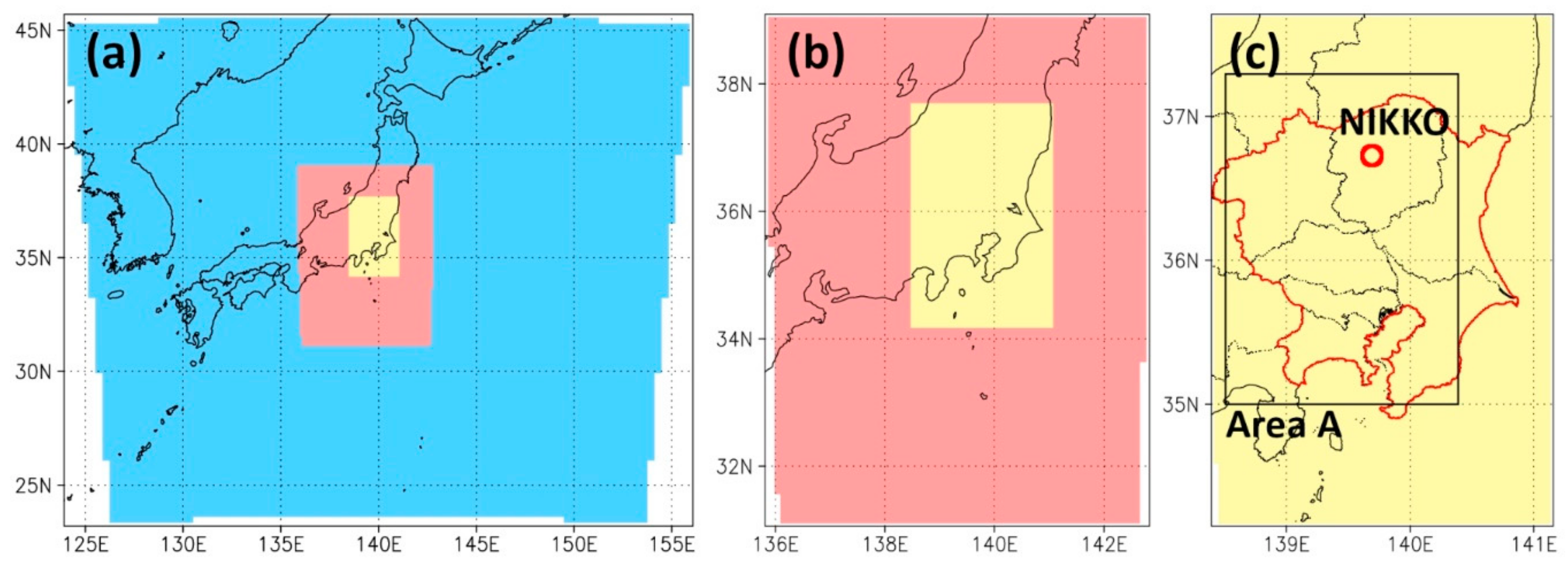
The Weather Research and Forecasting (WRF) model [19], Version 3.7.1, was used for numerical weather simulations. A two-way, three-level nesting was adopted, as shown in Figure 1. The spatial resolutions for the parent (D01), intermediate (D02), and child (D03) domains were 30 km, 10 km, and 3.333 km, respectively. Precipitation characteristics are investigated for the area indicated as Area A (138.5° E–140.4° E, 35.0° N–37.3° N) in Figure 1. The WRF single-moment 5 class scheme [20] and simplified Arakawa-Schubert scheme [21,22] were used for microphysics and cumulus parameterizations, respectively. The physical processes of the surface layer and land surface were calculated by the Eta model based on Monin-Obukhov with Zilitinkevich thermal roughness length [19] and the Noah land surface model [23], respectively. Planetary boundary layer processes were calculated using the Mello-Yamada-Janjic scheme [24]. For longwave and shortwave radiation, the simple rapid radiative transfer model [25] was used. Kinugawa heavy rainfall was affected by two typhoons. To compare the difference in precipitation caused by typhoons in a specific area under different climate conditions, the results of the simulations must have similar meteorological spatial distributions. Therefore, for D01, a spectral nudging method was applied for atmospheric temperature, zonal wind, meridional wind, and geopotential height every 6 h above a height of 6–7 km. An outline of these settings is given in

Table 2. Settings of the weather research and forecasting (WRF) simulations.

Item	Setting
Model version	3.7.1
Cloud microphysics	WRF single-moment 5 class scheme
Cumulus parameterization	Simplified Arakawa-Schubert scheme
Longwave and shortwave radiation	RRTM
Land surface scheme	Eta model
Land model	Noah land surface model
Planetary boundary layer scheme	Mellor-Yamada-Janjic
Settings of spectral nudging	Applied to the layer above 6–7 km for atmospheric temperature, zonal and meridional winds, and geopotential height

.

2.3. Non-Global Warming Conditions

To examine the impacts of global warming on an extreme weather event, hindcast and NGW simulations of the target event (e.g., Kinugawa heavy rainfall) were implemented in this study. In the NGW simulations, initial and boundary conditions are generated from a reanalysis and output of GCM projections. First, climatological monthly mean conditions of the historical experiment (${\overline{\mathbf{X}}}_H$) and historicalNat experiment (${\overline{\mathbf{X}}}_N$) are computed. Second, the difference between ${\overline{\mathbf{X}}}_N$ and ${\overline{\mathbf{X}}}_H$ is added to the reanalysis data, or NCEP FNL, ($X_{ANL}$). Then, the initial and boundary conditions for the NGW simulation ($X_{NGW}$) are calculated as follows:

$$X_{NGW}=X_{ANL}+\left({\overline{\mathbf{X}}}_N-{\overline{\mathbf{X}}}_H\right).$$

(1)

$X_{NGW}$ is generated from 6-hourly $X_{ANL}$. Therefore, the temporal variation in $X_{NGW}$ is similar to the actual condition ($X_{ANL}$), but the effects of global warming are removed in $X_{NGW}$. Thus, NGW simulations using $X_{NGW}$ produce possible variations in the target weather events under natural GHG emission conditions. In this study, ${\overline{\mathbf{X}}}_H$ and ${\overline{\mathbf{X}}}_N$ are computed as twenty-year averages from 1986 to 2005. NGW conditions were prepared for wind, atmospheric temperature, geopotential height, surface pressure, and specific humidity. The original values in NCEP FNL are given for relative humidity, and specific humidity for NGW conditions was generated from the original relative humidity and modified atmospheric temperature under NGW conditions. To prepare the SST for NGW conditions, the SST anomaly generated from the historical and historicalNat simulations in each GCM was added to the NOAA SSTs. Using the number in the 1st column of Table 1, an ensemble simulation based on each GCM output was named NGW-1, NGW-2, and so on.

2.4. Ensemble Simulation

To consider the chaotic behaviors of meteorological phenomena and uncertainties in the forcing data, an ensemble simulation technique is applied to numerical weather simulations. The lagged-simulated perturbation (LSP) method [26] was used for ensemble simulations. The LSP method was developed based on the lagged average forecasting (LAF) method [27]. The LSP method consists of three steps. First, three simulations are made from different initial times to generate three base state vectors ($S_1$, $S_2$, and $S_3$) at a certain interruption time. Second, the differences between $S_2$ and $S_1$ and between $S_3$ and $S_1$ are defined as difference vectors $\Delta S_2$ and $\Delta S_3$, respectively. Third, new state vectors ($S_n$) are generated from $S_1$, $\Delta S_2$ and $\Delta S_3$ as follows:

$$S_n=S_1+\alpha \Delta S_2+\beta \Delta S_3,$$

(2)

where α and β are the scale factors for $\Delta S_2$ and $\Delta S_3$, respectively. Then, simulations are restarted from the interruption time with the new state vectors $S_n$. In $S_n$, atmospheric temperature, zonal and wind components, specific humidity, atmospheric pressure, and SST are updated by the LSP method using the same scale factors for all variables. Nineteen ensemble members are produced for each ensemble simulation (1 hindcast and 12 NGW simulations) using the scale factors shown in

Table 3. Combination of scale factors (α and β) to produce the ensemble members in the lagged-simulated perturbation (LSP) method.

Combinations of Scale Factors (α and β)
(−1/3, 1/3)	(−1/3, 2/3)	(−1/3, 1)	(0, 1/3)
(0, 2/3)	(1/3, −1/3)	(1/3, 0)	(1/3, 1/3)
(1/3, 2/3)	(1/3, 1)	(2/3, −1/3)	(2/3, 0)
(2/3, 1/3)	(2/3, 2/3)	(1, −1/3)	(1, 1/3)

. The initial and interruption times of the simulations are shown in

Table 4. Initial and interruption times of the WRF simulation.

Run	Initial Time	Interruption Time (Generating New Ensemble Members)	End of Simulation
Run to make S1	00 UTC 7 September	00 UTC 8 September	00 UTC 11 September
Run to make S2	06 UTC 7 September
Run to make S3	12 UTC 7 September

.

3. Rainfalls in Hindcast and Non-Global Warming (NGW) Simulations

3.1. Validation of Hindcast Simulations

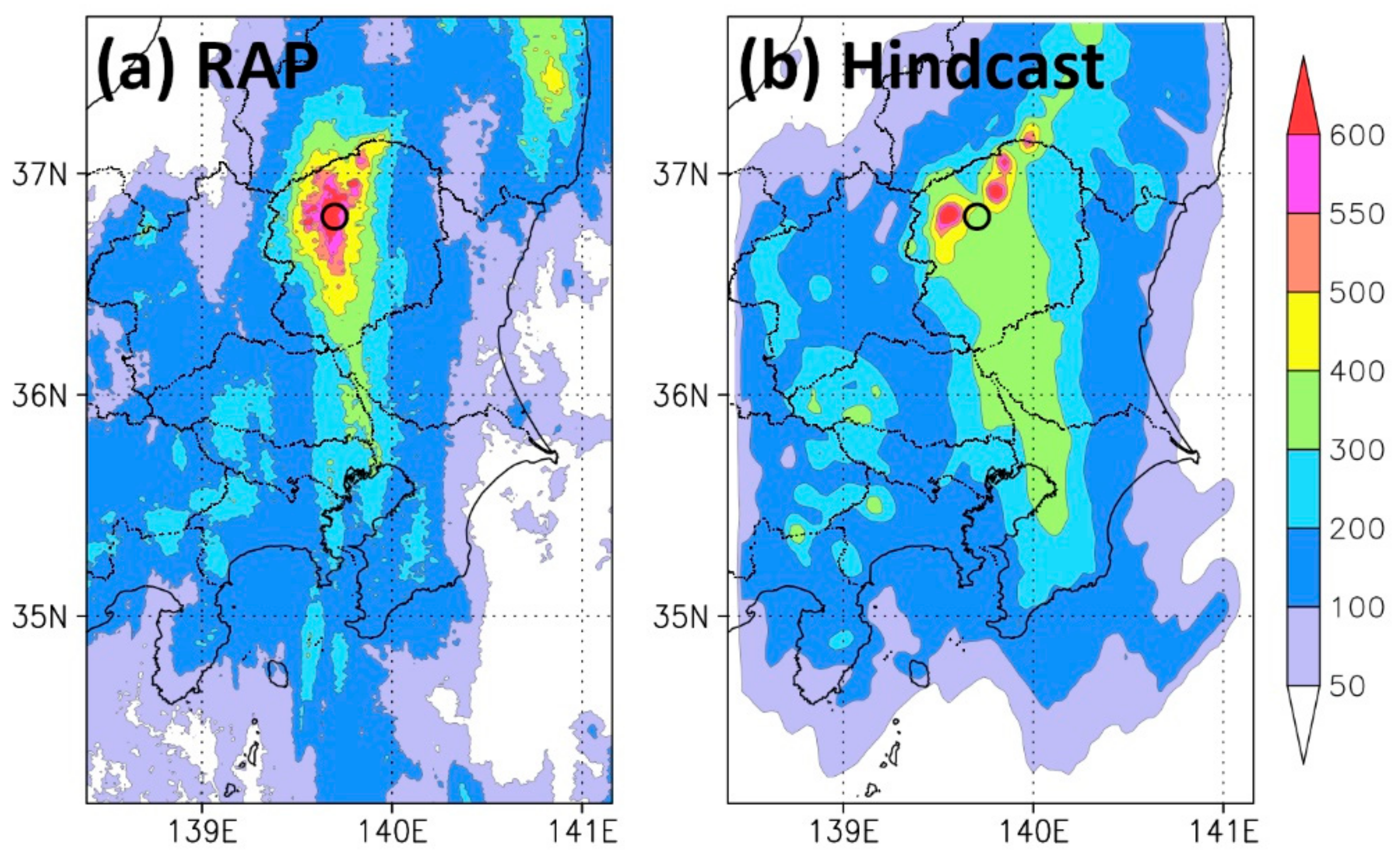
Figure 2 shows the total rainfall from 8 to 11 September 2015 by RAP and hindcast simulation. The hindcast result is an ensemble mean value of the 19 members. The RAP result shows the peak rainfall around Nikko city. The maximum observed total rainfall was 647.5 mm at Imaichi station. The area with total rainfall > 200 mm spread from approximately 35° N to 37.5° N. The size of the heavy rainfall system was larger than 200 km from south to north. In the hindcast, the peak of the total rainfall also emerged around Nikko city. However, the area with total rainfall > 400 mm was smaller than that of RAP, and several peaks were recognized. The maximum total rainfall was 760 mm for the ensemble mean result. For each member, the maximum total rainfall was from 624 to 976 mm. The north-south length of the heavy rainfall area was over 200 km in the hindcast. However, the area with total rainfall > 300 mm is much larger than that of RAP. Along 139° E, a certain amount of rainfall > 200 mm was found in the western part of the domain. There are some differences in the total rainfall between RAP and the hindcast, but the simulation result successfully captures the characteristics of the rainfall system.

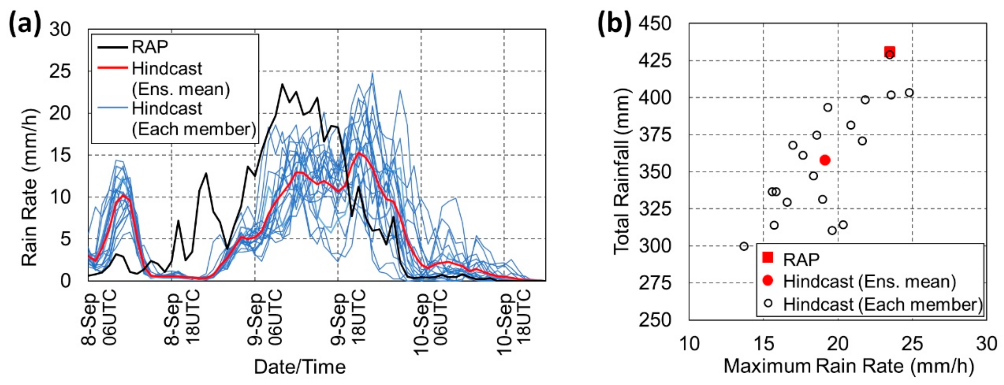
Figure 3a shows time-series of hourly rain rate averaged for the area around the Nikko city (139.5° E–140.0° E, 36.5° N–37.0° N). Ensemble mean result of the hindcast shows similar temporal pattern but slightly delays from the RAP result and the peak is smaller than the observation. In several members of the hindcast, the peak of the rain rate is comparable to the RAP result. Figure 3b is a scatter plot of the total rainfall and the maximum rain rate around the Nikko city. Ensemble mean total rainfall and the maximum rain rate are smaller than RAP. Several ensemble members show rain rate comparable to RAP. A single member shows the total rainfall is comparable to RAP, but even the minimum total rainfall is about 300 mm, and all the ensemble members generated significant rainfall around the Nikko city.

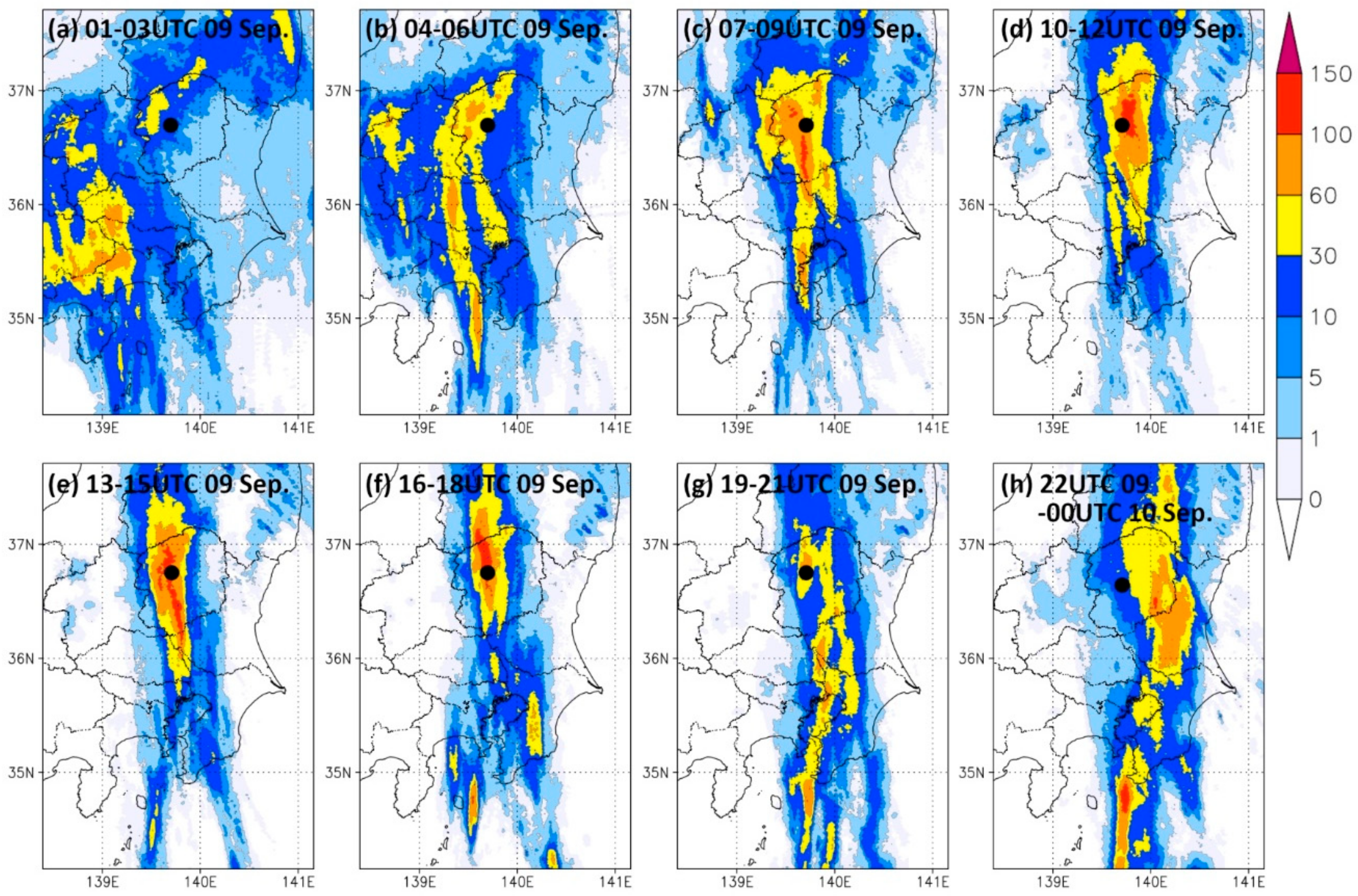
Figure 4 and Figure 5 show the 3-hourly rainfall by RAP and the hindcast. For the hindcast, the results of one member (a run began from 00 UTC 7 September) are shown. In RAP, the heavy rainfall area is located in the western part of D03 during the first 3 h (01–03 UTC 9 September). Then, the rainfall band moves eastward. The heavy rainfall band stays at approximately 139.7° E from 06 UTC 09 September to 21 UTC 9 September and then moves eastward again. Similar temporal variations in the location of heavy rainfall areas are recognized in the hindcast. Locations and rainfall rates were also comparable to RAP, but the size of the hindcast rainfall area was smaller than that of RAP before 12 UTC 9 September. After that, the sizes of both results are comparable. The same characteristics were found in other ensemble members of the hindcast simulation.

The results of the hindcast show that the characteristics for both the total amount and temporal variation in rainfall are similar to the actual condition. These results indicate the appropriateness of the WRF settings.

3.2. Comparison of Rainfall Characteristics between the Hindcast and NGW Simulations

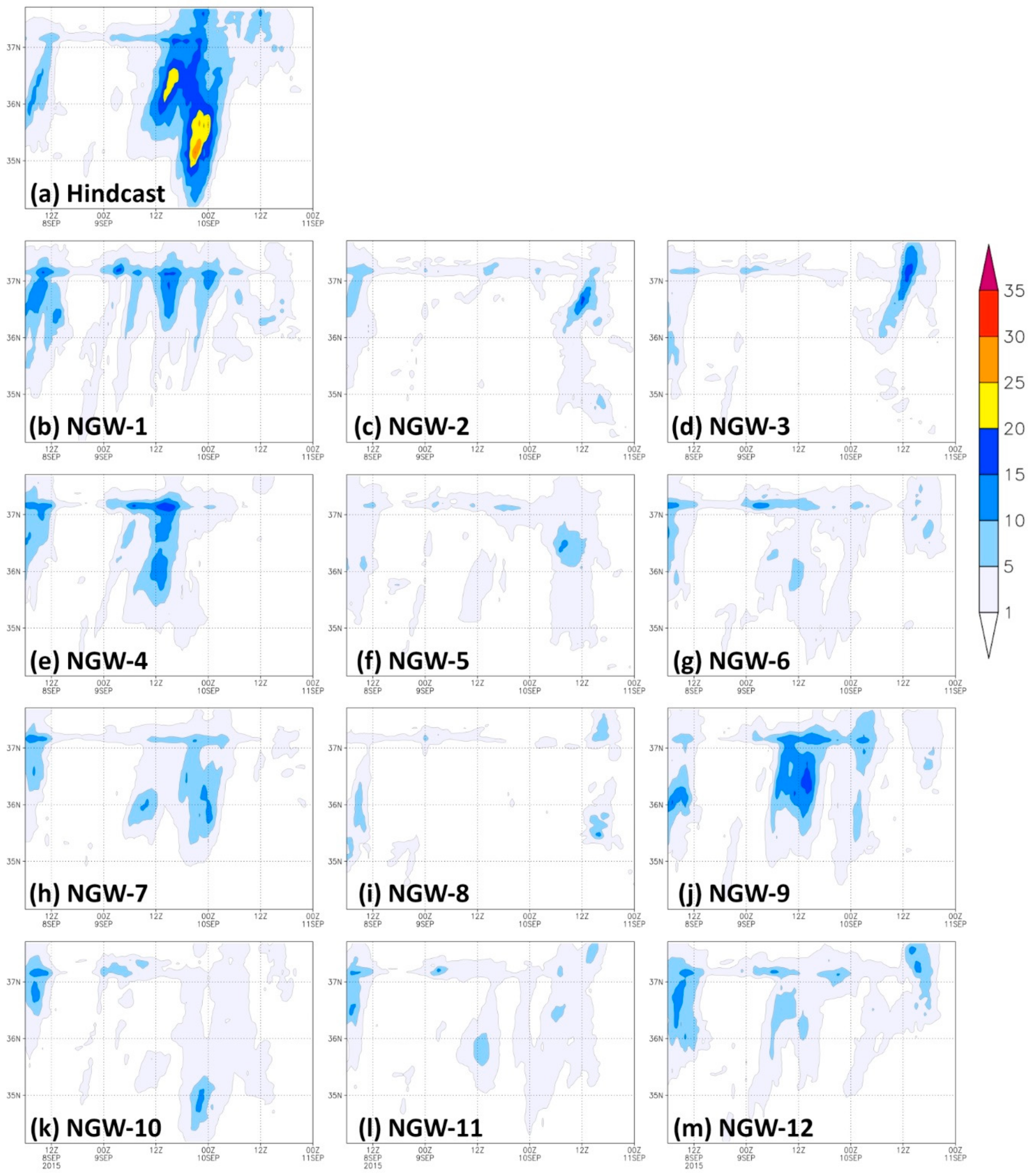
Figure 6 shows the total rainfall distribution by the 12 NGW simulations. Each result is the ensemble mean value of each NGW simulation. Except for NGW-8, significant total rainfall > 600 mm is found around Nikko city. In NGW-2, NGW-3, NGW-5, NGW-6, NGW-10, and NGW-11, the total rainfall in the western part of the domain is larger than that in the hindcast (Figure 2b). However, the total rainfall along 140° E is significantly smaller than that via the hindcast. In NGW-1, NGW-4, NGW-7, NGW-8, NGW-9, and NGW-12, the rainfall in the western part is comparable to the hindcast, but the rainfall is smaller along 140° E as seen in the other 6 NGW simulations. Figure 7 shows the latitude-time cross section of hourly rainfall. The results are the ensemble mean rainfall averaged for the 139.9° E–140.1° E band. In the hindcast, significant rainfall is recognized at approximately 12 UTC 09 September. Rainfall spreads southward, and a strong rainfall area is formed between 35° N and 36° N. This result indicates the development of a linear rainfall band in the hindcast from 12 UTC 9 September to 00 UTC 10 September. In NGW-1, NGW-4, NGW-7, and NGW-9, certain amounts of rainfall are recognized in this area, but they are smaller, and rainfall occurs in narrower areas than in the hindcast. In the other NGW simulations, weak or insignificant rainfall is found in this longitudinal area. The results of the NGW simulations indicate that the linear rainfall band is hardly generated or is not effectively developed under natural emission conditions.

Table 5. Total rainfall averaged for D03 (R_T,3).

Run	Average 1 (mm)	Max 2 (mm)	Min 3 (mm)	Standard Deviation (mm)
Hindcast	138	154	128	6.8
NGW-1	132 (−6)	142 (−12)	119 (−9)	6.1 (−0.7)
NGW-2	123 (−15)	136 (−18)	108 (-20)	7.2 (+0.4)
NGW-3	122 (−16)	134 (−20)	104 (−24)	7.4 (+0.6)
NGW-4	136 (−2)	147 (−7)	122 (−6)	6.7 (−0.1)
NGW-5	117 (−21)	124 (−30)	106 (−22)	4.8 (−2.0)
NGW-6	149 (+11)	167 (+13)	136 (+8)	7.4 (+0.6)
NGW-7	102 (−18)	111 (−43)	91 (−37)	4.9 (−1.9)
NGW-8	71 (−67)	77 (−77)	66 (−62)	2.7 (4.1)
NGW-9	134 (−4)	146 (−8)	122 (−6)	6.9 (+0.1)
NGW-10	128 (−10)	140 (−14)	118 (−10)	5.9 (−0.9)
NGW-11	113 (−25)	126 (−18)	102 (−26)	5.4 (−1.4)
NGW-12	125 (−13)	237 (+84)	107 (−21)	8.8 (+2.0)

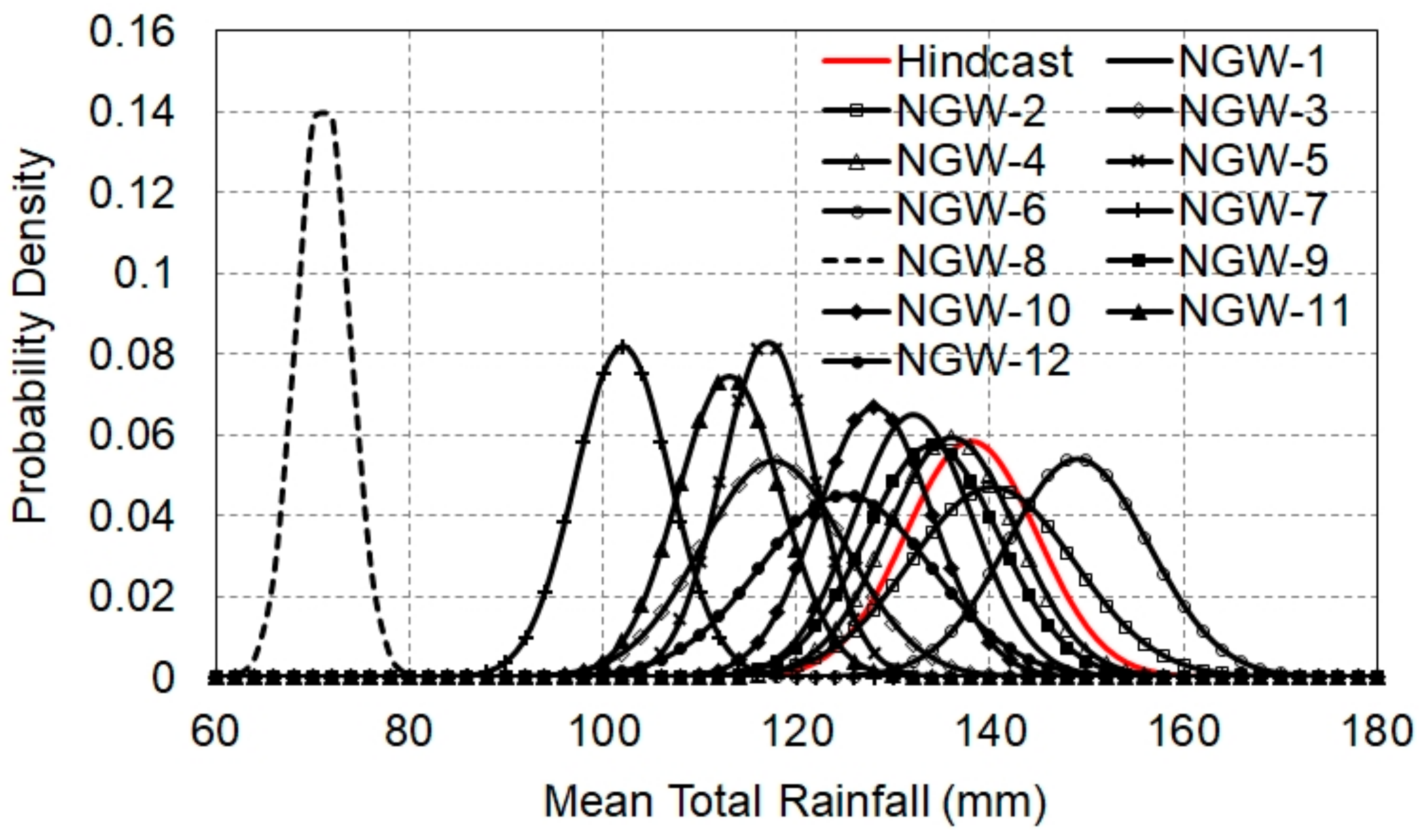
¹ Ensemble mean value of R_T,3. ² Maximum value of R_T,3 in the member of the hindcast and each NGW simulation. ³ Minimum value of R_T,3 in the member of the hindcast and each NGW simulation. Results of NGW simulations larger and smaller than the hindcast are shown in bold font and underlined, respectively. Values in parentheses are the difference between each NGW simulation and the hindcast.

is a summary of the total rainfall averaged for D03 (R_T,3). The mean and the maximum R_T,3 by the hindcast ensemble simulation are larger than those in 10 out of 12 NGW simulations. The minimum R_T,3 of the hindcast is larger than that in 11 NGW simulations. Figure 8 shows the probability density distribution of R_T,3 for the hindcast and NGW simulations. Probability density curves were estimated from the mean value and standard deviation of R_T,3 for the hindcast and NGW simulations based on a normal distribution assumption. The results of NGW-2 and NGW-6 indicate a high probability of the total rainfall being larger than the hindcast. The results of NGW-4 and NGW-9 are similar to those of the hindcast. The other 8 NGW simulations indicate a higher probability of rainfall smaller than the hindcast. The results in Table 5 and Figure 8 indicate a high probability of a larger amount of R_T,3 under the condition of higher GHG emissions.

Table 6. Total rainfall averaged for the area A (R_T,A).

Run	Average 1 (mm)	Max 2 (mm)	Min 3 (mm)	Standard Deviation (mm)
Hindcast	208	228	181	10.8
NGW-1	192 (−16)	214 (−14)	172 (−9)	11.9 (+1.1)
NGW-2	199 (−9)	222 (−6)	178 (−3)	13.7 (+2.9)
NGW-3	183 (−25)	204 (−24)	158 (−23)	11.1 (+0.3)
NGW-4	199 (−9)	215 (−13)	186 (+5)	8.1 (−2.7)
NGW-5	179 (−29)	193 (-35)	163 (−18)	6.5 (−4.3)
NGW-6	234 (+26)	261 (+33)	220 (+39)	11.2 (+0.4)
NGW-7	155 (−53)	167 (−61)	144 (−37)	5.2 (−5.6)
NGW-8	116 (−92)	129 (−99)	102 (−79)	6.0 (−4.8)
NGW-9	203 (−5)	228 (0)	180 (−1)	14.4 (+3.6)
NGW-10	191 (−17)	213 (−15)	176 (−5)	10.5 (−0.3)
NGW-11	174 (−34)	200 (−28)	160 (−21)	9.9 (−0.9)
NGW-12	191 (−17)	216 (−12)	160 (−21)	14.0 (+3.2)

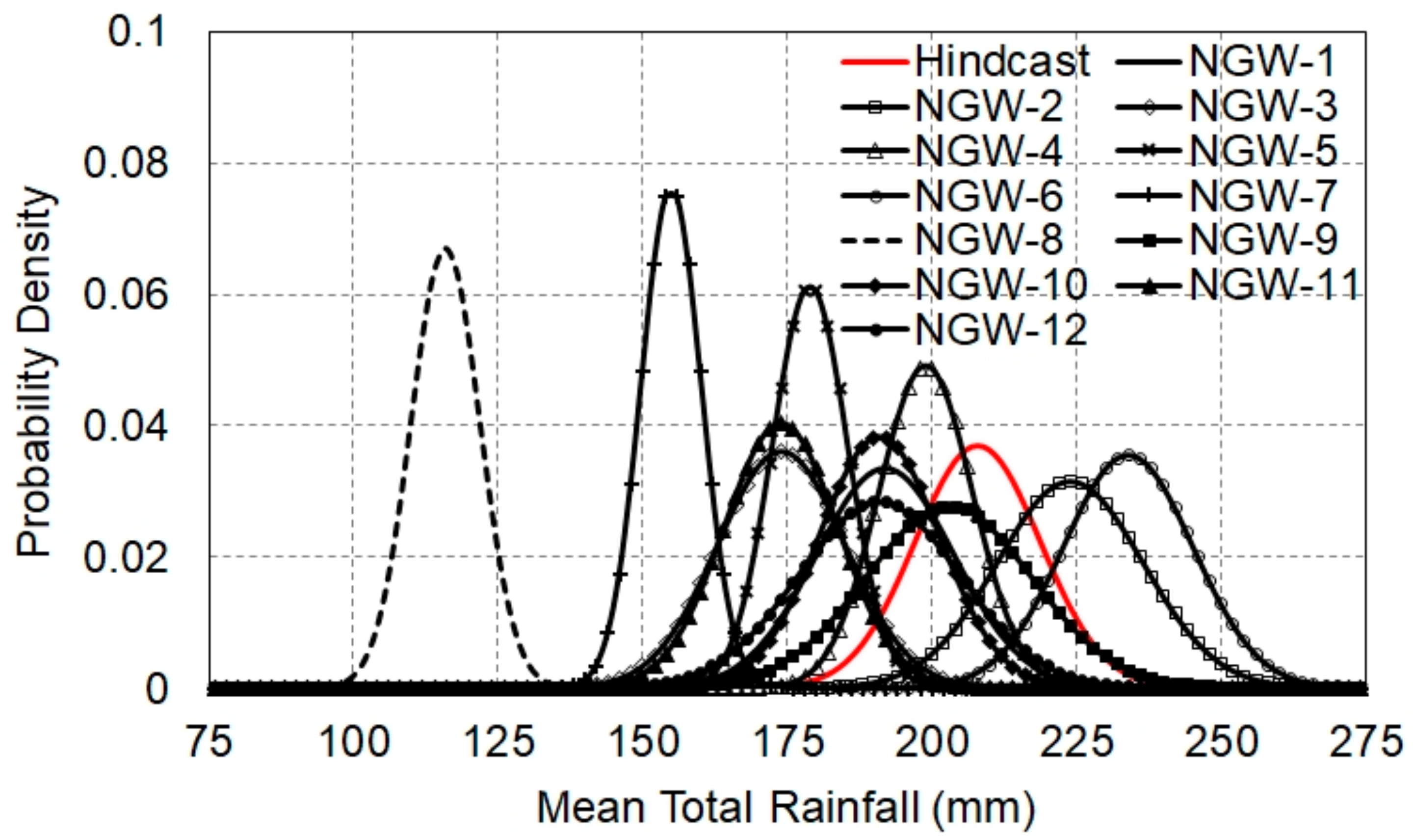
¹ Ensemble mean value of R_T,A. ² Maximum value of R_T,A in the member of the hindcast and each NGW simulation. ³ Minimum value of R_T,A in the member of the hindcast and each NGW simulation. Results of NGW simulations larger and smaller than the hindcast are shown in bold font and underlined, respectively. Values in parentheses are the difference between each NGW simulation and the hindcast.

and Figure 9 are the same results as Table 5 and Figure 8, respectively, but for the total rainfall averaged for area A (R_T,A). Area A is shown in Figure 1c. Except for NGW-6, the mean and maximum R_T,A are larger in the hindcast than in the 11 NGW simulations (Table 6). Figure 9 also shows that R_T,A is larger than it is in the natural emission scenario with high probability. These results indicate that the rainfall amount is larger under high GHG conditions, or that heavy rainfall is more severe in the hindcast not only for the wide area of the Kanto region (or D03) but also in the limited area.

Table 7. Ensemble mean values of the maximum hourly and 24-h rainfall.

Run	Hourly Rainfall	24-h Rainfall
Hindcast	120	554
NGW-1	118 (−2)	506 * (−48)
NGW-2	133 * (+13)	584 (+30)
NGW-3	119 (−1)	406 * (−148)
NGW-4	115 (−5)	543 (−11)
NGW-5	105 * (−15)	493 * (−61)
NGW-6	101 * (−19)	706 * (+152)
NGW-7	92 * (−28)	517 (−37)
NGW-8	110 (−10)	362 * (−192)
NGW-9	100 * (−20)	581 (+27)
NGW-10	102 * (−18)	514 (−40)
NGW-11	111 (−9)	580 (+26)
NGW-12	127 (+7)	540 (−14)

Results of NGW simulations larger and smaller than the hindcast are shown in bold font and underlined, respectively. NGW results with * indicate that difference from the hindcast is significant in 5% significance level. Values in parentheses are the difference between each NGW simulation and the hindcast.

shows the ensemble mean maximum hourly and 24-h rainfall for the hindcast and NGW simulations. Significance of the difference between the hindcast and each NGW simulation was examined by the Welch’s t-test. In 10 of the 12 NGW simulations, the maximum hourly rainfall is smaller than in the hindcast. However, only 5 NGW simulations show significant difference from the hindcast. Regarding the maximum 24-h rainfall, 8 from 12 NGW simulations showed larger values than in the hindcast, but 4 NGW simulations show significant difference. Only NGW-5 shows significant decrease in the average of the maximum hourly and 24-h rainfall. Results in Table 7 indicates that concentrated heavy rainfall under the high GHG condition could be stronger than under the natural GHG condition with high likelihood. For short-term heavy rainfall, the rainfall amount might be larger under the high GHG condition than the natural GHG condition.

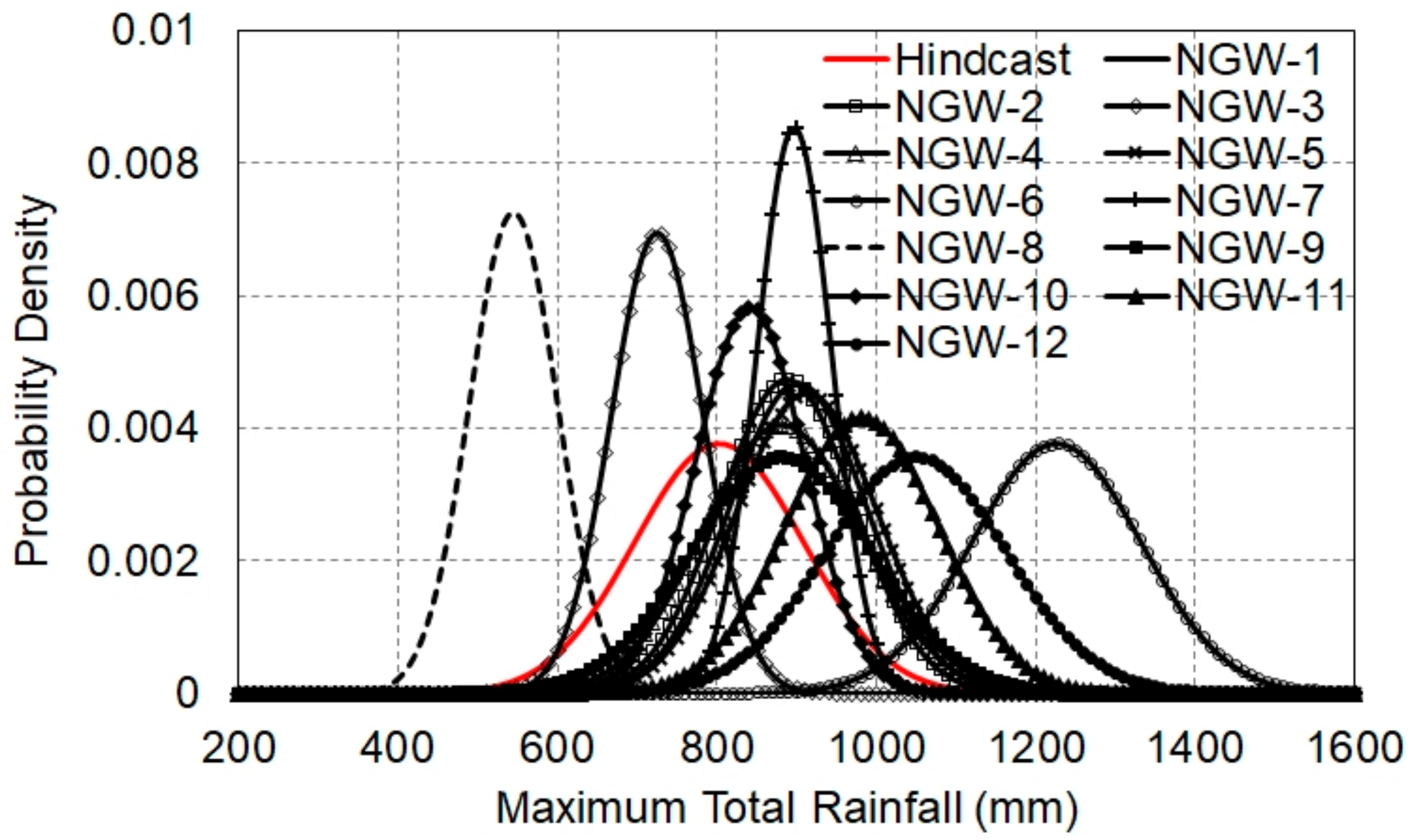
On the other hand, the maximum total rainfall is not necessarily larger under high GHG conditions. In all simulations, the maximum total rainfall is found around Nikko city (as seen in Figure 2 and Figure 6).

Table 8. The maximum total rainfall in D03 (R_MAX).

Run	Average 1 (mm)	Max 2 (mm)	Min 3 (mm)	Standard Deviation (mm)
Hindcast	803	976	624	106
NGW-1	902 (+99)	1102 (+126)	747 (+123)	85 (−21)
NGW-2	891 (+88)	1071 (+95)	790 (+166)	88 (−18)
NGW-3	742 (−61)	878 (−98)	639 (+15)	66 (−40)
NGW-4	881 (+78)	1061 (+85)	748 (+124)	98 (−8)
NGW-5	913 (+110)	1183 (+207)	806 (+182)	88 (−18)
NGW-6	1226 (+423)	1391 (+415)	1002 (+378)	106 (0)
NGW-7	897 (+94)	970 (−6)	783 (+159)	47 (−59)
NGW-8	545 (−258)	670 (−306)	433 (−191)	55 (−51)
NGW-9	881 (+78)	1114 (+138)	686 (+62)	112 (+6)
NGW-10	842 (+39)	999 (+23)	746 (+122)	69 (−37)
NGW-11	984 (+181)	1107 (+131)	787 (+163)	96 (−10)
NGW-12	1080 (+277)	1232 (+256)	860 (+236)	112 (+6)

¹ Ensemble mean value of R_MAX. ² Maximum value of R_MAX in the member of the hindcast and each NGW simulation. ³ Minimum value of R_MAX in the member of the hindcast and each NGW simulation. Results of NGW simulations larger and smaller than the hindcast are shown in bold font and underlined, respectively. Values in parentheses are the difference between each NGW simulation and the hindcast.

and Figure 10 show the same results as Table 5 and Figure 8, respectively, but for the maximum total rainfall (R_MAX) in D03. The ensemble mean R_MAX of the hindcast is larger than that of NGW-3 and NGW-8 but smaller than that of the other 10 NGW simulations. The maximum value of R_MAX for the hindcast is larger than that of only 3 of the NGW simulations (NGW-3, NGW-7, and NGW-8). The minimum R_MAX of the hindcast is larger than that for only 1 NGW simulation (NGW-8). Figure 10 shows that R_MAX is not necessarily larger in the hindcast than in the NGW simulations. In contrast, R_MAX values in some NGW simulations are clearly larger than those in the hindcast.

In the next section, the atmospheric conditions and SST of the hindcast and NGW simulations are investigated to discuss the causes and mechanisms of differences in rainfall between the hindcast and NGW simulations.

4. Atmospheric Conditions and Sea Surface Temperature (SSTs) for Hindcast and NGW Simulations

In the previous section, rainfall characteristics were compared between the hindcast and NGW simulations. In this section, atmospheric conditions are examined to reveal the causes and mechanisms of differences in rainfall between high GHG emissions and natural emission conditions.

Figure 11 shows the difference in atmospheric temperature 2 m above the Earth’s surface (T2) under initial conditions between each NGW simulation and the hindcast. In NGW-2, NGW-4, and NGW-8, T2 is almost the same as, or higher than, in the hindcast over a wide area. Under warmer atmospheric conditions, saturated water vapor pressure is larger than under cooler conditions, and more precipitable water content (PWC) is expected in the atmosphere. However, the total rainfall in D03 and area A for NGW-2, NGW-4, and NGW-8 were the same or smaller than those in the hindcast. In NGW-10, T2 is partly higher than in the hindcast to the north of D01. However, the total rainfall in D03 and area A is smaller than that in the hindcast. In other NGW simulations, T2 is lower than it is in the hindcast in all part of D01. As seen in Figure 8 and Figure 9, the total rainfall amounts in D03 and area A for NGW-6 were larger than those in the hindcast, but the result in Figure 11 shows a smaller T2, which is not favorable for larger rainfall.

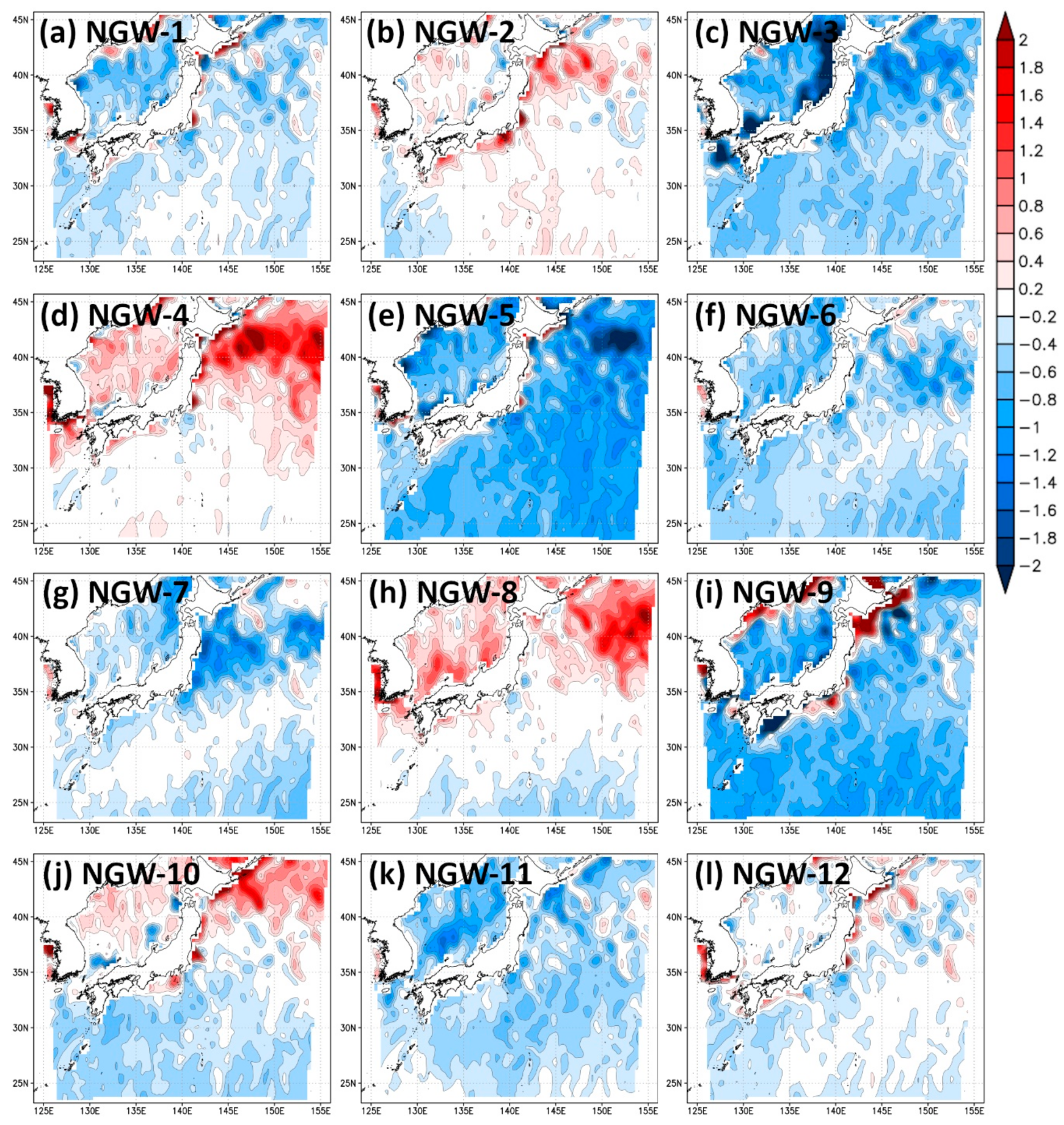
Figure 12 is the same as Figure 11, but for SST. In NGW-2, NGW-4, NGW-8, and NGW-10, a significant increase in SST is recognized in the northern part of the domain. These warmer areas correspond to those of T2 in each NGW simulation. These results indicate that the SST anomaly could cause a warmer T2. However, as seen in Figure 11, there is no positive SST anomaly in NGW-6, in which the total rainfall tends to be larger than the hindcast. In NGW-2, in which the total rainfall is slightly larger than the hindcast, a warmer SST anomaly is found on the south coast of the Japan main island. However, significant positive SSTs in NGW-4, NGW-8, and NGW-10 do not cause more rainfall in the Kinugawa basin.

Figure 13 is the same as Figure 11 but for PWC. In NGW-2, NGW-4, and NGW-8, PWC is larger in a certain area of the target domain. These positive anomalies of PWC correspond to those of T2 and SST. However, a positive PWC anomaly is found in a limited area in NGW-10, which shows a higher T2 and SST in the north region of the target domain. A positive PWC anomaly of NGW-2 (but not NGW-4 and NGW-8) could cause larger total rainfall. In NGW-6 (the case of the largest R_T,3 and R_T,A), PWC is not clearly larger than the hindcast value.

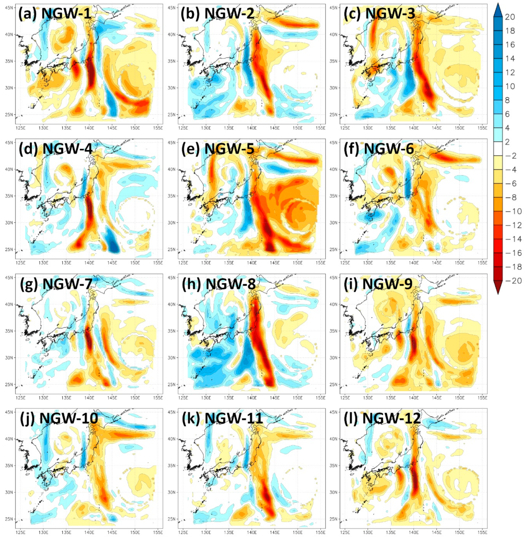
The results in Figure 11, Figure 12 and Figure 13 indicate that anomalies under the initial conditions cannot explain the variations in rainfall. Figure 14 shows the PWC anomaly at 18 UTC 9 September. At this time, heavy rainfall is found in the Nikko region, and a linear rainfall band is formed along 140° E (Figure 2, Figure 6, and Figure 7). Spatial patterns of PWC anomalies are affected by atmospheric flow according to typhoons 17 and 18. In NGW-1, a negative PWC anomaly (or drier atmospheric condition) is found in a wide area of D01, but a higher PWC compared to the hindcast value is found in some parts. Not only climatological anomalies found under initial conditions but also such atmospheric conditions caused by each meteorological event result in variations in rainfall. In NGW-4, a negative PWC anomaly is found at a longitude of 140° E, in which heavy rainfall occurs in the hindcast (Figure 2). Then, even with no significant variation in SST and PWC at the initial time, the rainfall amount decreased in NGW-4. In NGW-8, a positive PWC anomaly is widely spread in the western part of D01, but there is a significant decrease in PWC along 140° E. As seen in Figure 13, there is a higher PWC in NGW-8 under the initial condition compared with the hindcast, but the northward flow along typhoon 17 brought a drier air mass into the area around the Kinugawa basin; therefore, the total rainfall amount in NGW-8 is smaller than that in the hindcast.

In

Table 9. Spatial mean PWC and divergence for area A at 18 UTC 9 September. Values in parentheses are the difference between each NGW simulation and the hindcast. The result values are the ensemble mean for the hindcast and each NGW simulation.

Run	PWC (mm)	Divergence (10−5/s)
Hindcast	40.3	−1.05
NGW-1	35.6 (−4.7)	0.88 (+1.93)
NGW-2	43.7 (+3.4)	−1.23 (−0.17)
NGW-3	39.8 (−0.5)	−0.70 (+0.36)
NGW-4	40.1 (−0.2)	0.69 (+1.74)
NGW-5	40.7 (+0.4)	−0.59 (+0.46)
NGW-6	43.8 (+3.5)	0.04 (+1.09)
NGW-7	36.2 (−4.1)	1.07 (+2.12)
NGW-8	36.2 (−4.1)	0.63 (+1.67)
NGW-9	38.9 (−1.4)	−0.15 (+0.90)
NGW-10	42.2 (+1.9)	0.20 (+1.25)
NGW-11	41.5 (+1.2)	0.59 (+1.64)
NGW-12	36.4 (−3.9)	0.54 (+1.60)

, the spatial mean PWC at 18 UTC 9 September for area A is shown for the hindcast and NGW simulations. In many NGW simulations, the PWC in area A is smaller than that in the hindcast, and the total rainfall also tends to be smaller than that in the hindcast (Figure 9). In the cases of NGW-2 and NGW-6, where the total rainfall in area A tends to be larger than that via the hindcast, the PWC is higher than it in the hindcast and other NGW simulations. However, the PWCs in NGW-5, NGW-10, and NGW-11 are larger than those in the hindcast, but the total rainfall is not necessarily larger compared to the hindcast.

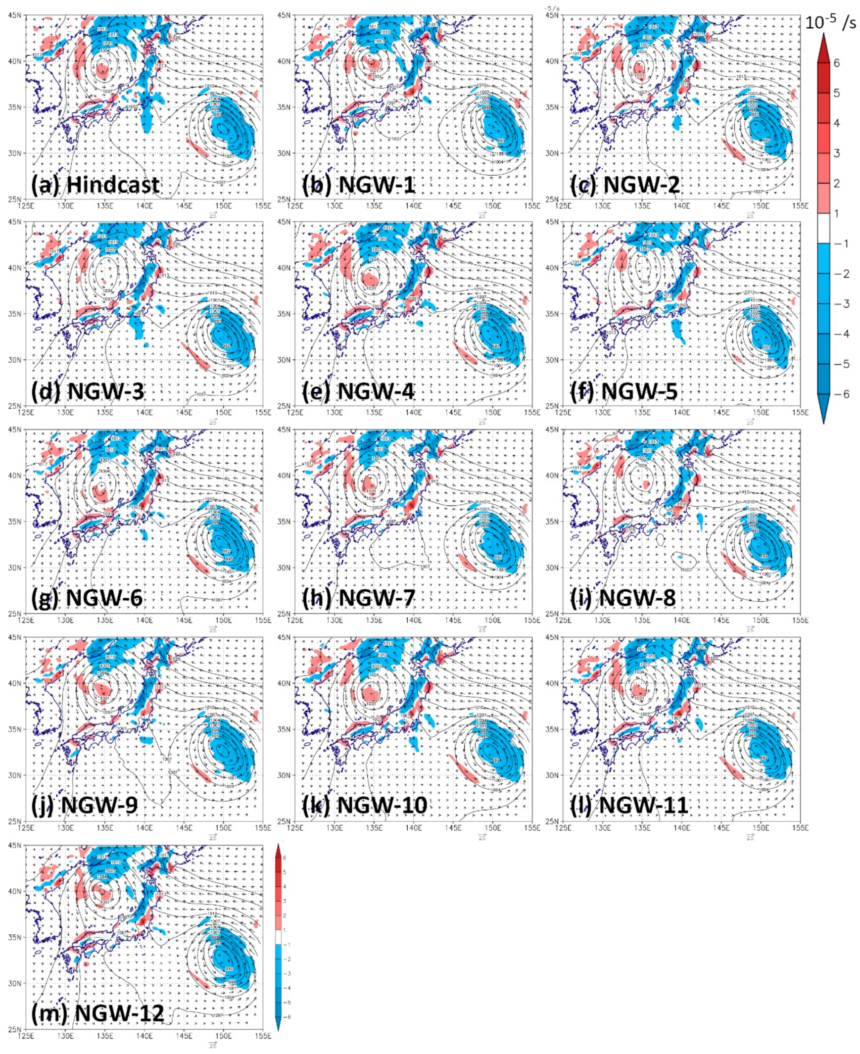
Figure 15 shows the spatial distributions of divergence, wind, and sea level pressure at 18 UTC 9 September. Divergence and wind are averaged for the layers from 1000 hPa to 700 hPa. In the hindcast, a negative value (or convergence) is found around the Kinugawa basin. In NGW-2, NGW-3, and NGW-5, negative values are recognized around the Kanto area. In other NGW simulations, positive values or no clear tendency (divergence or convergence) are found in the Kanto area. The spatial mean divergence for area A is shown in Table 9. Negative values are found in the hindcast, NGW-2, NGW-3, NGW-5, and NGW-8. In NGW-2, a higher PWC and stronger convergence compared to the hindcast resulted in more rainfall. In NGW-5, NGW-10, and NGW-11, the PWC is greater than it is in the hindcast, but convergence is weaker than it is in the hindcast. Therefore, the rainfall value is smaller than it is in the hindcast. The convergence tendency is weaker in NGW-6, but the PWC is much higher than it is in the hindcast (largest in all NGW simulations). Then, total rainfall is larger than it is in the hindcast.

Weaker convergence in the NGW simulations could explain other characteristics of rainfall. In many NGW simulations, the maximum total rainfall is larger than that in the hindcast (Figure 10). However, the area with total rainfall >300 mm is smaller than it is in the hindcast (Figure 6). The weaker convergence conditions could not generate rain bands in the southern Kanto area (Figure 7), and water vapor derived from the Pacific Ocean was not consumed in the southern part of the Kanto area and flowed northward into the Nikko area. Then, heavy orographic rainfall was generated in the upper Kinugawa basin, and was larger than it was in the hindcast.

In the case of Kinugawa heavy rainfall in 2015, another concern is whether the two typhoons were stronger under the high GHG condition (or in the hindcast).

Table 10. Ensemble means of the minimum central pressures of typhoons 17 and 18.

Run	Typhoon 17	Typhoon 18
Hindcast	977.4	988.1
NGW-1	978.0	989.7
NGW-2	976.4	987.6
NGW-3	976.8	987.8
NGW-4	976.4	985.8
NGW-5	979.1	990.4
NGW-6	977.1	985.5
NGW-7	978.3	988.6
NGW-8	976.9	992.1
NGW-9	977.6	988.9
NGW-10	977.2	987.5
NGW-11	977.1	989.3
NGW-12	976.7	988.5

Values smaller than the results of the hindcast are underlined.

shows the minimum central pressures of typhoons 17 and 18 for the hindcast and NGW simulations. In NGW-2, the minimum central pressure is lower than it is in the hindcast for both typhoons 17 and 18. Such intensification of the typhoons could cause stronger convergence in NGW-2 (Table 9). However, NGW-3. NGW-4, NGW-6, and NGW-10 indicate the intensification of the two typhoons, but the convergence in area A is weaker than that in the hindcast. Other NGW simulations show weaker typhoon activity with unclear tendencies. These results indicate that the difference in typhoon activity has an insignificant impact on heavy rainfall around the Kanto region in the case of Kinugawa heavy rainfall in 2015.

5. Conclusions

In this study, an EA method combined with an ensemble simulation technique was adopted to investigate impacts of anthropogenic GHG emissions on an extreme heavy rainfall event in the Kinugawa basin. The results of the hindcast and NGW simulations showed that the ensemble mean total rainfall around the Kanto area in the hindcast is larger than that in most of the NGW simulations. The probability density of the spatial mean total rainfall indicated a high likelihood of larger rainfall in the hindcast than in the NGW simulations. Hourly and 24-h rainfall in the hindcast are also larger than they are in most of the NGW simulations. The time-latitude cross section of rainfall showed the development of a linear rainfall band in the hindcast but no strong rainfall band in the NGW simulations. These results indicate the high probability of intensification of Kinugawa heavy rainfall by anthropogenic GHG emissions. However, a few NGW simulations showed greater rainfall than in the hindcast. In addition, the maximum total rainfall of the NGW simulations in the target domain tended to be larger than it was in the hindcast. To reveal the causes of larger rainfall in the NGW simulations, atmospheric conditions and SST were investigated. The initial atmospheric and SST conditions showed colder and drier conditions in many NGW simulations. Warmer and wetter conditions were found in some NGW simulations. However, such atmospheric conditions at the initial time did not always correspond to the difference of simulated rainfall characteristics. The simulated atmospheric conditions (PWC and horizontal divergence) during heavy rainfall well explained the variations in rainfall in the NGW simulations (Table 8). In particular, the divergent conditions (or weaker convergence) in the southern part of the Kanto area could not cause linear rainfall band in the NGW simulations. In the cases of weak rainfall in the southern Kanto area, water vapor would not be consumed, and a moist air mass could flow into the northern part of the region by the strong wind around the typhoon. Such a rich moisture inflow could cause the larger maximum total rainfall in the NGW simulations.

The results of this study indicate that heavy rainfall in Kinugawa could be enhanced by anthropogenic GHG emissions. However, anomalous climatological conditions (or differences in the initial conditions of the numerical simulations) cannot always explain the impacts of anthropogenic GHGs on extreme heavy rainfall events. For understanding the processes and reasons for variations in rainfall characteristics, a detailed analysis of the simulation results is vital.

Another result of this study is the comparison of typhoon activity between the hindcast and NGW simulations. There was no significant intensification of typhoon 17 during the Kinugawa heavy rainfall event due to anthropogenic GHG emissions. The results in this study indicate that the record-breaking heavy rainfall around the Kinugawa basin in 2015 was mainly caused by the increase in PWC along with a higher atmospheric temperature, but there was no clear difference in the role of the typhoon. If typhoon activities are intensified under a future climate, it would cause more severe heavy rainfall, similar to the Kinugawa heavy rainfall. A pseudo global warming technique would be useful for the assessment of future extreme events and disaster prevention planning.

References

- Bindoff, N.L.; Stott, P.A.; AchutaRao, K.M.; Allen, M.R.; Gillett, N.; Gutzler, D.; Hansingo, K.; Hegerl, G.; Hu, Y.; Jain, S.; et al. Detection and Attribution of Climate Change: From Global to Regional. In Climate Change 2013: The Physical Science Basis; Contribution of Working Group I to the Fifth Assessment Report of the Intergovernmental Panel on Climate Change; Stocker, T.F., Qin, D., Plattner, G.-K., Tignor, M., Allen, S.K., Boschung, J., Nauels, A., Xia, Y., Bex, V., Midgley, P.M., Eds.; Cambridge University Press: Cambridge, UK; New York, NY, USA, 2013. [Google Scholar]
- National Academies of Sciences, Engineering, and Medicine. Attribution of Extreme Weather Events in the Context of Climate Change; The National Academies Press: Washington, DC, USA, 2016. [Google Scholar] [CrossRef] [Green Version]
- Otto, F.E.L.; Massey, N.; van Oldenborgh, G.J.; Jones, R.G.; Allen, M.R. Reconciling two approaches to attribution of the 2010 Russian heat wave. Geophys. Res. Lett. 2012, 39. [Google Scholar] [CrossRef] [Green Version]
- Eden, J.M.; Kewb, S.F.; Bellpratc, O.; Lenderinkb, G.; Manolad, I.; Omranie, H.; van Oldenborgh, G.J. Extreme precipitation in the Netherlands: An event attribution case study. Weather Clim. Extrem. 2018, 21, 90–101. [Google Scholar] [CrossRef]
- Wilcox, L.J.; Yiou, P.; Hauser, M.; Lott, F.C.; van Oldenborgh, G.J.; Colfescu, I.; Dong, B.; Heger, G.; Shaffrey, L.; Sutton, R. Multiple perspectives on the attribution of the extreme European summer of 2012 to climate change. Clim. Dyn. 2017, 50, 3537–3555. [Google Scholar] [CrossRef] [Green Version]
- Shiogama, H.; Watanabe, M.; Imada, Y.; Mori, M.; Kamae, Y.; Ishii, M.; Kimoto, M. Attribution of the June–July 2013 Heat Wave in the Southwestern United States. SOLA 2014, 10, 122–126. [Google Scholar] [CrossRef] [Green Version]
- Shiogama, H.; Watanabe, M.; Imada, Y.; Mori, M.; Kamae, Y.; Ishii, M.; Kimoto, M. An event attribution of the 2010 drought in the South Amazon region using the MIROC5 model. Atmos. Sci. Lett. 2013, 14, 170–175. [Google Scholar] [CrossRef]
- Christidis, N.; Stott, P.A. Change in the Odds of Warm Years and Seasons Due to Anthropogenic Influence on the Climate. J. Clim. 2014, 27, 2607–2621. [Google Scholar] [CrossRef]
- Takayabu, I.; Hibino, K.; Sasaki, H.; Shiogama, H.; Mori, N.; Shibutani, Y.; Takemi, T. Climate change effects on the worst-case storm surge: A case study of Typhoon Haiyan. Environ. Res. Lett. 2015, 10, 064011. [Google Scholar] [CrossRef]
- Xu, Z.; Yang, Z.-L. Relative impacts of increased greenhouse gas concentrations and land cover change on the surface climate in arid and semi-arid regions of China. Clim. Chang. 2017, 144, 491–503. [Google Scholar] [CrossRef]
- Patricola, C.M.; Wehner, M.F. Anthropogenic influences on major tropical cyclone events 2018. Nature 2018, 563, 339–346. [Google Scholar] [CrossRef] [Green Version]
- Trenberth, K.E.; Fasullo, J.T.; Shepherd, T.G. Attribution of climate extreme events. Nat. Clim. Chang. 2015, 5, 724–730. [Google Scholar] [CrossRef]
- Shepherd, T.G. A Common Framework for Approaches to Extreme Event Attribution. Curr. Clim. Chang. Rep. 2016, 2, 28–38. [Google Scholar] [CrossRef] [Green Version]
- NCEP GDAS/FNL 0.25 Degree Global Tropospheric Analyses and Forecast Grids. Available online: https://rda.ucar.edu/datasets/ds083.3/ (accessed on 19 January 2020).
- Reynolds, R.W.; Smith, T.M.; Liu, C.; Chelton, D.B.; Casey, K.S.; Schlax, M.G. Daily high-resolution-blended analyses for sea surface temperature. J. Clim. 2007, 20, 5473–5496. [Google Scholar] [CrossRef]
- Taylor, K.E.; Stouffer, R.J.; Meehl, G.A. An overview of CMIP5 and the experiment design. Bull. Am. Meteorol. Soc. 2012, 93, 485–498. [Google Scholar] [CrossRef] [Green Version]
- Makihara, Y.; Uekiyo, N.; Tabata, A.; Abe, Y. Accuracy of Radar-AMeDAS Precipitation. IEICE Trans. Commun. 1996, 79, 751–762. [Google Scholar]
- CMIP5 Models and Grid Resolution. Available online: https://portal.enes.org/data/enes-model-data/cmip5/resolution (accessed on 10 January 2020).
- Skamarock, W.C.; Klemp, J.B.; Dudhia, J.; Gill, D.O.; Barker, J.M.; Duda, M.G.; Huang, X.-Y.; Wang, W.; Powers, J.G. A description of the advanced research WRF Version 3. No. NCAR/RN-475+STR. NCAR Tech. Notes 2008, 113. [Google Scholar] [CrossRef]
- Lin, Y.-L.; Farley, R.D.; Orville, H.D. Bulk parameterization of the snow field in a cloud model. J. Appl. Meteorol. Climatol. 1983, 22, 1065–1092. [Google Scholar] [CrossRef] [Green Version]
- Pan, H.-L.; Wu, W.-S. Implementing a Mass Flux Convection Parameterization Package for the NMC Medium-Range Forecast Model; NMC Office Note 409; National Center for Environmental Prediction: College Park, MD, USA, 1995; Volume 409, p. 40. [Google Scholar]
- Arakawa, A.; Schubert, W.H. Interaction of a Cumulus Cloud Ensemble with the Large-Scale Environment, Part I. J. Atmos. Sci. 1974, 31, 674–701. [Google Scholar] [CrossRef] [Green Version]
- Chen, F.; Dudhia, J. Coupling an advanced land surface-hydrology model with the Penn State-NCAR MM5 modeling system. Part I: Model implementation and sensitivity. Mon. Weather Rev. 2001, 129, 569–585. [Google Scholar] [CrossRef] [Green Version]
- Jianjic, Z. The Step-Mountain Eta Coordinate Model: Further Developments of the Convection, Viscous Sublayer, and Turbulence Closure Schemes. Mon. Weather Rev. 1994, 122, 927–945. [Google Scholar] [CrossRef] [Green Version]
- Dudhia, J. Numerical Study of Convection Observed during the Winter Monsoon Experiment Using a Mesoscale Two-Dimensional Model. J. Atmos. Sci. 1989, 46, 3077–3107. [Google Scholar] [CrossRef]
- Taniguchi, K. A Simple Ensemble Simulation Technique for Assessment of Future Variations in Specific High-Impact Weather Events. J. Geophys. Res. Atmos. 2018, 123, 3443–3461. [Google Scholar] [CrossRef]
- Hoffman, R.N.; Kalnay, E. Lagged average forecasting, an alternative to Monte Carlo forecasting. Tellus A 1983, 35, 100–118. [Google Scholar] [CrossRef]
Figure 1.
Target domains for the weather research and forecasting (WRF) simulations. (a) Parent domain; (b) intermediate domain; (c) child domain. The blue, red, and yellow areas represent the parent, intermediate, and child domains, respectively. The red line and open rectangle shown in (c) indicate the Kanto area and area A, respectively. The red circle in (c) is the location of Nikko city.
Figure 2.
Total rainfall from 8 to 11 September 2015. (a) Result by Radar-AMeDAS precipitation (RAP); (b) ensemble mean total rainfall of the hindcast. Open circle indicates the location of the Nikko city. The unit of the color bar is mm.
Figure 3.
(a) Time-series of hourly rain rate averaged for the area around the Nikko city; (b) scatter plot of the maximum rain rate and total rainfall averaged for the area around the Nikko city.
Figure 4.
3-hourly rainfall by Radar-AMeDAS precipitation (RAP). Result of (a) 01–03 UTC, (b) 04–06 UTC, (c) 07–09 UTC, (d) 10–12 UTC, (e) 13–15 UTC, (f) 16–18 UTC, (g) 19–21 UTC on 9 September. (h) Result of 22 UTC on 9 September–00 UTC on 10 September. The unit of the color bar is mm/3 h. Filled black circle indicate the location of the Nikko city.
Figure 5.
3-hourly rainfall by the hindcast simulation (a member starts at 00 UTC 7 September). Result of (a) 01–03 UTC, (b) 04–06 UTC, (c) 07–09 UTC, (d) 10–12 UTC, (e) 13–15 UTC, (f) 16–18 UTC, (g) 19–21 UTC on 9 September. (h) Result of 22 UTC on 9 September–00 UTC on 10 September. The unit of the color bar is mm/3 h. Filled black circle indicate the location of the Nikko city.
Figure 6.
Spatial distribution of the ensemble mean total rainfall in D03 for non-global warming (NGW) simulations. Result of (a) NGW-1, (b) NGW-2, (c) NGW-3, (d) NGW-4, (e) NGW-5, (f) NGW-6, (g) NGW-7, (h) NGW-8, (i) NGW-9, (j) NGW-10, (k) NGW-11, (l) NGW-12. The unit of the color bar is mm. Open circle indicates the location of the Nikko city.
Figure 7.
Latitude-time cross section of hourly rainfall averaged for the 139.9° E–140.1° E band. Ensemble mean values are shown for each panel. Result of (a) hindcastm, (b) NGW-1, (c) NGW-2, (d) NGW-3, (e) NGW-4, (f) NGW-5, (g) NGW-6, (h) NGW-7, (i) NGW-8, (j) NGW-9, (k) NGW-10, (l) NGW-11, (m) NGW-12. The unit of the color bar is mm/h.
Figure 8.
Probability density curves of the mean total rainfall for D03 (RT,3). The horizontal axis is RT,3 (mm). The vertical axis is the probability density.
Figure 9.
Probability density curves of the mean total rainfall for area A (RT,A). The horizontal axis is RT,3 (mm). The vertical axis is the probability density.
Figure 10.
Probability density curves of the maximum total rainfall in D03 (RMAX). The horizontal axis is RMAX (mm). The vertical axis is the probability density.
Figure 11.
Difference in atmospheric temperature 2 m above the Earth’s surface under initial conditions between each NGW simulation and the hindcast. Result (a) NGW-1, (b) NGW-2, (c) NGW-3, (d) NGW-4, (e) NGW-5, (f) NGW-6, (g) NGW-7, (h) NGW-8, (i) NGW-9, (j) NGW-10, (k) NGW-11, (l) NGW-12. The unit of the color bar is Kelvin.
Figure 12.
Difference in sea surface temperature (SST) under initial conditions between each NGW simulation and the hindcast. Result of (a) NGW-1, (b) NGW-2, (c) NGW-3, (d) NGW-4, (e) NGW-5, (f) NGW-6, (g) NGW-7, (h) NGW-8, (i) NGW-9, (j) NGW-10, (k) NGW-11, (l) NGW-12. The unit of the color bar is Kelvin.
Figure 13.
Difference in precipitable water content (PWC) under initial conditions between each NGW simulation and the hindcast. Result (a) NGW-1, (b) NGW-2, (c) NGW-3, (d) NGW-4, (e) NGW-5, (f) NGW-6, (g) NGW-7, (h) NGW-8, (i) NGW-9, (j) NGW-10, (k) NGW-11, (l) NGW-12. The unit of the color bar is mm.
Figure 14.
Difference in PWC at 18 UTC 9 September between each NGW simulation and the hindcast. Result of (a) NGW-1, (b) NGW-2, (c) NGW-3, (d) NGW-4, (e) NGW-5, (f) NGW-6, (g) NGW-7, (h) NGW-8, (i) NGW-9, (j) NGW-10, (k) NGW-11, (l) NGW-12. The unit of the color bar is mm.
Figure 15.
Spatial distribution of divergence (shaded), wind (arrows), and sea level pressure (contours) at 18 UTC 9 September. Divergence and wind are averaged for the layers from 1000 to 700 hPa. Result (a) hindcast, (b) NGW-1, (c) NGW-2, (d) NGW-3, (e) NGW-4, (f) NGW-5, (g) NGW-6, (h) NGW-7, (i) NGW-8, (j) NGW-9, (k) NGW-10, (l) NGW-11, (m) NGW-12. The unit of the color bar is 10−5 /s.