Article

Model Inter-Comparison for PM2.5 Components over urban Areas in Japan in the J-STREAM Framework

by
Kazuyo Yamaji
1,*,
Satoru Chatani
2,
Syuichi Itahashi
3,
Masahiko Saito
4,
Masayuki Takigawa
5,
Tazuko Morikawa
6,
Isao Kanda
7,
Yukako Miya
8,
Hiroaki Komatsu
9,
Tatsuya Sakurai
10,
Yu Morino
2,
Kyo Kitayama
2,
Tatsuya Nagashima
2,
Hikari Shimadera
11,
Katsushige Uranishi
11,
Yuzuru Fujiwara
12,
Tomoaki Hashimoto
12,
Kengo Sudo
13,
Takeshi Misaki
1,14 and
Hiroshi Hayami
3
1
Graduate School of Maritime Sciences, Kobe University, Kobe, Hyogo 658-0022, Japan
2
National Institute for Environmental Studies, Tsukuba, Ibaraki 305-8506, Japan
3
Central Research Institute of Electric Power Industry, Abiko, Chiba 270-1194, Japan
4
Ehime University, Matsuyama, Ehime 790-8566, Japan
5
Japan Agency for Marine—Earth Science and Technology, Yokohama, Kanagawa 236-0001, Japan
6
Japan Automobile Research Institute, Tsukuba, Ibaraki 305-0822, Japan
7
Japan Meteorological Corporation, Osaka 556-0021, Japan
8
Japan Weather Association, Toshima, Tokyo 170-6055, Japan
9
Kanagawa Environmental Research Center, Hiratsuka, Kanagawa 254-0014, Japan
10
School of Science and Engineering, Meisei University, Hino, Tokyo 191-8506, Japan
11
Graduate School of Engineering, Osaka University, Suita, Osaka 565-0871, Japan
12
Suuri-Keikaku, Chiyoda, Tokyo 101-0003, Japan
13
Graduate School of Environmental Studies, Nagoya University, Nagoya, Aichi 464-8601, Japan
14
Tokyo Electric Power Services Co., Ltd., Koto, Tokyo 135-0062, Japan
*
Author to whom correspondence should be addressed.
Submission received: 14 January 2020 / Revised: 14 February 2020 / Accepted: 19 February 2020 / Published: 25 February 2020

Abstract

:
A model inter-comparison of secondary pollutant simulations over urban areas in Japan, the first phase of Japan’s study for reference air quality modeling (J-STREAM Phase I), was conducted using 32 model settings. Simulated hourly concentrations of nitric oxide (NO) and nitrogen dioxide (NO2), which are primary pollutant precursors of particulate matter with a diameter of 2.5 µm or less (PM2.5), showed good agreement with the observed concentrations, but most of the simulated hourly sulfur oxide (SO2) concentrations were much higher than the observations. Simulated concentrations of PM2.5 and its components were compared to daily observed concentrations by using the filter pack method at selected ambient air pollution monitoring stations (AAPMSs) for each season. In general, most models showed good agreement with the observed total PM2.5 mass concentration levels in each season and provided goal or criteria levels of model ensemble statistics in warmer seasons. The good performances of these models were associated with the simulated reproducibility of some dominant components, sulfates (SO42−) and ammonium (NH4+). The other simulated PM2.5 components, i.e., nitrates (NO3), elemental carbon (EC), and organic carbon (OC), often show clear deviations from the observations. The considerable underestimations (approximately 30 µg/m3 for total PM2.5) of all participant models found on heavily polluted days with approximately 40–50 µg/m3 for total PM2.5 indicated some problems in the simulated local meteorology such as the atmospheric stability. This model inter-comparison suggests that these deviations may be owing to a need for further improvements both in the emission inventories and additional formation pathways in chemical transport models, and meteorological conditions also require improvement to simulate elevated atmospheric pollutants. Additional accumulated observations are likely needed to further evaluate the simulated concentrations and improve the model performance.

1. Introduction

Particulate matter (PM) consists of a complex mixture of solid and liquid particles of organic and inorganic substances suspended in the atmosphere. The major components of PM are sulfates (SO42−), nitrates (NO3), ammonium (NH4+), sodium chloride (NaCl), black carbon (BC) or elemental carbon (EC), organic carbon (OC), mineral dust, and water. The PMs with the greatest negative health effects are those with a diameter of 2.5 µm or less (PM2.5), which can penetrate and lodge deep inside the lungs [1]. Some PMs are also climate-dependent, known as short-lived climate pollutants (SCLPs) [2]. Warming due to sunlight absorption (e.g., BC) and cooling due to sunlight scattering (e.g., SO42−) directly affect radiative forcing in the earth’s climate system. Additionally, water-soluble PMs affect the regional climate system interacting with cloud microphysics. These radiative and microphysical interactions can induce changes in regional precipitation and atmospheric circulation patterns. Some PM2.5 particles are directly emitted from natural sources and human activities, while others are formed through complex oxidation reactions and particle agglomeration. Combining the regional three-dimensional chemical transport model (CTM) with comprehensive particulate formations may be a useful tool for understanding the detailed behavior of short-lived PM2.5 components in the atmosphere.
Recently, PM2.5 air quality has been improved in East Asian countries, e.g., China [3] and Japan [4]; however, PM2.5 concentrations at Japanese air pollution monitoring stations (APMSs) have not met yet the environmental quality standard, defined as 15 µg/m3 for the annual PM2.5 mean and 35 µg/m3 for 24-h PM2.5 mean, or the World Health Organization (WHO) air quality guidelines, with corresponding values of 10 and 35 µg/m3. An established reference regional CTM system should be applied to design effective PM2.5 control strategies [5]. However, accurately reproducing or predicting the concentrations and distributions of PM2.5 and its relevant substances remains challenging, due to inaccurate emission inventories, poorly represented initial and boundary conditions, imperfect physical, dynamical, and chemical parameterizations, and limited observations for verification, as noted for previous Asian scale model inter-comparisons, i.e., the model inter-comparison study for Asia (MICS-Asia) series [6,7,8,9] and the urban air quality model inter-comparison study in Japan (UMICS) series [10,11,12].
A model inter-comparison framework, Japan’s study for reference air quality modeling (J-STREAM), was designed to establish a reference regional CTM system to consider strategies for reducing PM2.5 and its relevant substances [5]. In this paper, the capacities of participant models for J-STREAM to simulate PM2.5 and its components were evaluated for two urban areas in Japan in each season. The model improvements will be discussed based on the inter-model differences.

2. Methodology

2.1. Framework of J-STREAM Phase I

A model inter-comparison project in Japan, J-STREAM, was initiated in 2016. One aim of J-STREAM is to investigate differences in simulated concentrations of secondary atmospheric pollutants such as PM2.5 components and ozone over urban areas in Japan due to differences between model frames and/or model settings, including boundary and inputted conditions and physical and chemical mechanisms. Detailed model settings are described below. Furthermore, these including an introduction of J-STREAM can be found in previous research for the overview [5] and the performance on ozone [13].
The main target of the first phase of J-STREAM (J-STREAM Phase I) is to evaluate the general performances of participant models on secondary atmospheric concentrations over urban areas in Japan. Daily concentrations of PM2.5 components in each season among others were treated as subjects of evaluation in this paper. The enhanced simulation periods of J-STREAM Phase I were the spring of 2013, 27 April–26 May 2013, the summer of 2013, 12 July–10 August 2013, the autumn of 2013, 11 October–9 November 2013, and the winter of 2014, 10 January–8 February 2014, which corresponded to the seasonal periods of the national observation frame for PM2.5 components (Table 1). The detailed evaluations and additional experiments for individual participant models can be found in [14].
Four nested model domains, d01, d02, d03, and d04, on a Lambert conformal map projection were employed in the J-STREAM project [5]. The finest domains, d03 and d04, with a 5 × 5 km grid, cover the major city clusters in western Japan, including Osaka, Kobe, Kyoto, and Nagoya, and the Tokyo metropolitan area, respectively. Simulated concentrations in the d03 and d04 domains were used for model evaluations, and the results are discussed in following sections. Figure 1 shows the d03 and d04 domains, including the locations of ambient APMSs (AAPMSs), for which simulated concentrations were evaluated via comparisons with observations.

2.2. Baseline Meteorological Model Configurations

The baseline meteorological simulation for J-STREAM Phase I was performed by the Weather Research and Forecasting (WRF) model, using the Advanced Research WRF (ARW) Version 3.7.1 [15]. The WRF inputted data were acquired from the National Centers for Environmental Prediction Final Operational Model Global Tropospheric Analyses (ds083.2) with a 1 × 1 degree resolution [16] and the Real-Time, Global Sea Surface Temperature High-Resolution (RTG_SST_HR) analysis with a 1/12 × 1/12 degree resolution [17] and a temporal resolution of 6 h for the initial and boundary conditions. The horizontal configurations of the one-way nested model domains, d01, d02, d03, and d04, are 220 × 170 grids with a 45-km horizontal resolution, 154 × 160 grids with a 15-km resolution, 82 × 61 grids with a 5-km resolution, and 64 × 70 grids with a 5-km resolution, respectively. The vertical grid structure consists of 31 layers from the surface to the model top (100 hPa). Five grids were trimmed off each of the four lateral boundaries for the offline CTMs. The physics parameterizations applied in this model included the WRF Single-Moment 5-class scheme [18], the Radiative Transfer Model (RRTM) [19] for a longwave radiation scheme, the Dudhia scheme [20] for a shortwave radiation scheme, the Noah Land Surface Model [21], the Mellor-Yamada Nakanishi and Niino surface layer scheme level 2.5 [22], and the Kain-Fritsch convective parameterization [23] for d01 and d02. No convection parameterization was used for the 5-km domains. The grid-nudging four-dimensional data assimilation technique was employed for wind, temperature, and water vapor from level 11 (approximately 2 km) to the top of the model at 100 hPa with the nudging coefficients of 1.0 × 10⁻⁴ and 0.5 × 10⁻⁵ s−1 for d01 and d02, respectively. Most of the participant CTMs employed baseline meteorological fields, while others employed the meteorology based on different model settings. The differences in the model settings in some participant models are described in Section 2.3.
The baseline meteorological fields were compared with hourly observations of the Japan Meteorological Agency (JMA) for the observation stations within d03 and d04 (Figure 1) over four seasons: the spring of 2013 (11–26 May 2013), the summer of 2013 (27 July–10 August 2013), the autumn of 2013 (25 October–9 November 2013), and the winter of 2014 (24 January–7 February 2014) (Figure 2 and Figure 3). The hourly observed and modeled meteorological variables were averaged for all meteorological observatories for each domain.
The WRF using the baseline setting can generally simulate the observed meteorological conditions well. Meanwhile, WRF tended to overestimate the observed wind speeds. This was likely affected by the sparse horizontal resolution and coarse land information. The simulation performance of wind patterns was slightly better for d04 than that for d03 (Figure 2 and Figure 3). However, simulated precipitation timing and their amounts were consistent with the observations (Figure 2 and Figure 3).

2.3. Chemical Transport Model Configurations

A total of 32 simulations were performed using three types of regional CTMs in J-STREAM Phase I: Community Multiscale Air Quality (CMAQ) [24], Comprehensive Air quality Model with eXtensions (CAMx) [25], and Weather Research and Forecasting-Chemistry (WRF-Chem) [26]. Table 2 presents the configurations of the employed models. All participants conducted J-STREAM simulation under their own usual simulation conditions. The CMAQ group (M01–M28) included several versions, i.e., chemical mechanisms: Statewide Air Pollution Research Center mechanism (SAPRC) 99 [27], SAPRC07 [28], Carbon Bond (CB) 05 [29], and Regional Atmospheric Chemistry Mechanism (RACM) 2 [30], and three types of CMAQ aerosol calculation techniques [31]: aero5, aero6, and aero6 with the volatility basis set (VBS) approach [32]. These CMAQ aerosol calculation techniques employed ISORROPIA Version 1 [33,34] as an aerosol thermodynamic model and the second version of ISORROPIA (ISORROPIA Version 2) for updating the crustal species thermodynamics, the speciation schemes, and the SO42− formation pathway [35] for versions after 5.0. The basic techniques of aero5 and aero6 include secondary organic aerosol (SOA) formation processes based on empirical parameters for SOA yields [36]. Major or minor updates were reflected in the chemical and aerosol mechanisms in the later versions. One CAMx model (M29) applied in J-STREAM used the SAPRC07 chemistry and the coarse and fine aerosol scheme treating both static coarse and fine mode aerosols [37]. The WRF-Chem group (M30–M32) included two Versions (3.8.1 and 3.7.1) that employed RADM2: the aerosol module of the Modal Aerosol Dynamics Model for Europe (MADE) [38] and the SOA Model (SORGAM) [39].
As described in detail in an overview article on J-STREAM [5], participants were requested to run CTM simulations during the enhanced target periods of four seasons for d03 or d04. As shown in Table 2, the simulations for some participant models began at d01 (M02, M03, M07–M15, M20, and M30–M32), but others began from the more inner domains. Fifteen participant models (M01–07, M14, M15, M21–M24, M26, M29, and M30) submitted their results for both domains for all four seasons, but the other participants submitted results for only selected seasons, with the highest number of model results for the summer of 2013.
Initial concentrations on the first day of each season and boundary concentrations throughout the entire target period were generated in the simulation using the M15 setting via CMAQ Version 5.0.2 with the SAPRC07–aero6 mechanisms for d01 and d02. Boundary concentrations for d01 of M15 were obtained from results for a chemical atmospheric general circulation model designed for studying atmospheric environment and radiative forcing, CHASER [40] for the Hemispheric Transport of Air Pollution (HTAP) Version 2 [41]. In J-STREAM Phase I, model-ready mosaic emission data corresponding to all participant chemical–aerosol mechanisms involving multiple emission inventories and results from an emission model for biogenic volatile organic compounds were provided: HTAP Version 2.2 [42] and Global Fire Emissions Database Version 4.1 [43] for Asian anthropogenic emissions, the Japan Auto–Oil Program (JATOP) emission inventory database (JEI-DB) [44], the updated JEI–DB [5], and Sasakawa Peace Foundation emissions for ships for Japanese anthropogenic emissions, volcanic emission data from Aerosol Comparisons between Observations and Models (AeroCom) [45] and JMA [46], and estimations obtained by using Model of Emissions of Gases and Aerosols from Nature Version 2.1 [47]. Most participant CTMs used model-ready input data; however, some participant CTMs performed simulations in their own emission frames. M03 used EAGrid2010-JAPAN [48], and M20 and M27 used EAGrid2000-JAPAN [49] for anthropogenic emissions in Japan. For the Asian scale anthropogenic emissions, M20 employed NASA INTEX-B [50] instead of HTAP Version 2.2. Additionally, some CTMs employed different emission injection heights. The Model for Ozone and Related chemical Tracers Version 4 (MOZART-4) [51], for instance, was used as boundary conditions in some model settings.
As mentioned in Section 2.2., most of the participants employed the baseline meteorological fields; however, other CTMs (M07, M20) used WRF-ARW outputs based on their own conditions, including physical options, parameterizations, and a fine input meteorological analysis data, which is the grid point value derived from the mesoscale model (GPV MSM) data by JMA.

3. Observational Data for Model Evaluation

A monitoring framework of ambient PM2.5 components was initiated in the fiscal year 2011 under the Japan government initiative [4]. Over a period of at least two weeks set for each season, 1-day accumulated concentrations of PM2.5 components, including ions (e.g., SO42−, NO3, and NH4+), inorganic elements (e.g., Na, Al, K, and Ca), and carbonaceous aerosols (EC and OC), were monitored using the filter pack method at selected stations from three types of APMSs, including AAPMSs, roadside APMSs (RAPMSs), and background monitoring stations (BGMSs). PM2.5 mass concentrations determined gravimetrically by weighing the filters were employed as the PM2.5 mass concentration in this paper. Monitoring data from valid AAPMSs that obtained data for each PM2.5 component over a period of at least eight days (53%) from each target period (up to 15 days) per each station were used to evaluate the performances of the participant CTMs. The number of valid AAPMSs was 16–22 stations for each domain and season. The data acquisition rate was highest in the summer, while a poor data acquisition rate was found for NO3 in autumn. Observed gaseous pollutants at these AAPMSs were also used to evaluate the simulated nitric oxide (NO), nitrogen dioxide (NO2), and sulfur dioxide (SO2).
Figure 4 and Figure 5 present observed daily concentrations for PM2.5 components, i.e., SO42−, NO3, NH4+, EC, and OC, and total PM2.5 mass for each 12- to 15-day seasonal period at the AAPMSs for d03 and d04, respectively. The box-and-whisker and black dots (outliers) means the differences between AAPMSs in each domain.
In general, the concentrations of the total PM2.5 and its components within a single domain exhibit similar day-to-day variabilities for each season. However, the frequency distributions of daily concentrations between the AAPMSs in each domain were enhanced, particularly for elevated concentrations (Figure 4 and Figure 5). Therefore, the spatially averaged concentrations obtained from daily monitoring data for different AAPMSs within each domain were used for time series analysis hereafter.
For d03, i.e., western Japan, the seasonal-average total PM2.5 concentrations were 17.3, 23.1, 20.3, and 19.6 µg/m3, with maximum daily concentrations of 31.9, 37.6, 36.3, and 34.3 µg/m3 for spring, summer, autumn, and winter. The summer PM2.5 concentration was slightly higher than those for the other seasons; however, the seasonal characteristics of the PM2.5 concentration are unclear. SO42− was a dominant PM2.5 component, accounting for approximately 40% (9.1 µg/m3) of the total PM2.5 mass concentration in the summer. Meanwhile, from autumn to winter, the ratios of NO3and OC to total PM2.5 mass increased. The ratios of the five major PM2.5 components were similar, with values of 12%–19% in the winter. On the dates when PM2.5 was elevated, the AAPMS differences in PM2.5 concentration levels increased, and considerably high PM2.5 was found at AAPMSs placed at major cities: Osaka and Nagoya. These results were compared with those from rural areas.
For d04, the Tokyo metropolitan area, which is several hundred kilometers east of d03, the day-to-day changes in the concentrations of total PM2.5 and its components were similar to those for d03; however, the seasonal-average concentrations: 15.2, 18.6, 17.9, and 19.3 µg/m3 for spring, summer, autumn, and winter, were slightly lower than those for d03; whereas the maximum daily concentrations were 26.3, 35.4, 41.9, and 46.8 µg/m3. The elevated daily concentrations were obviously higher than those for d03 in the autumn and winter. Wintertime PM2.5 concentrations were slightly higher than those in the other seasons, with increased daily concentrations; however, the seasonal characteristics of the PM2.5 concentration were unclear for d04. The daily variabilities of the total PM2.5 mass were characterized by SO42− in spring and summer, where the ratios of SO42− to total PM2.5 mass were 32% (4.8 µg/m3) and 39% (4.8 µg/m3), respectively. In autumn, the ratios of the other PM2.5 components, including OC, NO3, and NH4+, to the total PM2.5 mass increased. The OC and NO3concentrations were both higher than the SO42− concentration in winter. In particular, for the first pollutant peak on 25 January, OC and NO3 were dominant, accounting for 22% (9.2 µg/m3) and 23% (9.6 µg/m3) of the total PM2.5 mass concentration, respectively. For the peak on 2 February, NO3 was dominant, accounting for 22% (9.2 µg/m3). SO42− was the dominant PM2.5 component throughout the year for d03, but for d04, OC and NO3 levels were higher than SO42− levels in the winter. On the dates PM2.5 elevated, the AAPMSs differences of PM2.5 concentration levels were increased, and the considerably high PM2.5 were found at the AAPMSs placed on the central area of d04, i.e., the Tokyo metropolitan area.

4. Results and Discussion

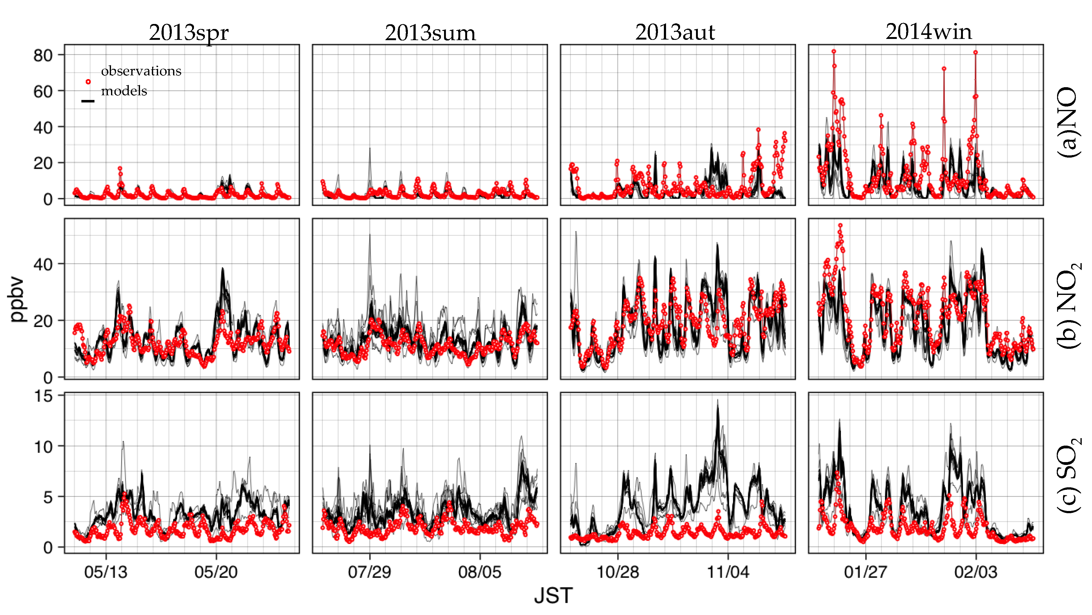
4.1. Hourly Concentrations of Primary Pollutants

Major gaseous pollutants were also monitored at the AAPMSs. Figure 6 and Figure 7 present the spatial averages of observed and simulated hourly concentrations of NO, NO2, and SO2 from different AAPMSs for d03 and d04, respectively. Table 3 summarizes the ensemble performances of the participant CTMs at each AAPMS for each season.
In general, most CTMs showed good agreement with the observed concentration levels of NO and NO2 for each season, with regular diurnal patterns of NO in the warmer seasons. However, none of the models fully reproduced the elevated concentrations, e.g., for 19–20 May and 3 November (NO and NO2) and 30 January (NO), with differences of 50%–200% between the observations and models, among others; the models tend to overestimate the observed daily maximums of NO: around 10–20 ppbv in spring and around 10–30 ppbv in summer, by a factor of 2.
For midnight on 30 January, all participant CTMs could not simulate the considerably increased level of NO before the rapid NO decrease associated with airmass changes, although all participants reproduced the NO decrease well. This suggests that CTMs successfully simulated the concentration change owing to meteorological changes in the synoptic scale but failed to simulate an increase in the amounts owing to local scale meteorological changes such as the strong atmospheric stability, especially during colder seasons. All models tended to overevaluate the daytime NO reduction. In particular, two WRF-Chem types (M30 and M31) and M05 produced strikingly low constant values, 0.001 or 0.000 ppbv, during the daylight hours in summer and autumn. The normalized mean bias (NMB) for both domains produced a strong underestimation of NO (approximately −40% to −50%), except during the spring. Underestimates of NO at remote stations in Japan have been observed for regional CTMs, as reported by MICS–Asia III results [9], and the correlations and index of agreement (IoA) values ranged from 0.18 to 0.43 and 0.41 to 0.51, respectively. The performance levels of each model exhibited substantial differences between both domains and seasons. The differences between seasons are likely related to meteorology simulation abilities, but the reasons for the differences appearing between domains are unclear in this stage.
The differences for NO2 in each model were large. Among these models, M31, M32, and M30 tended to overestimate elevated NO2 levels. The lower levels of NO2 obtained by M30 were often comparable to the NO2 concentration obtained by M03, which provided considerably lower NO2 concentrations compared to other models. These results suggest that the differences in meteorological conditions and NOx chemistry in each model produced the NO2 discrepancy between the models. Most of the models produced better results for NO2 than for NO, with ensemble averages of seasonal statistics, e.g., correlation values, of 0.56 (d03) and 0.55 (d04), 0.72 (d03), and 0.71 (d04), particularly in the winter.
Over the year, most models obviously overestimated the observed SO2, with an ensemble bias of 1.7–4.2 ppbv (NMB: 120%–350%) for d03 and 1.5–2.5 ppbv (NMB: 160%–470%) for d04. In addition, relatively high SO2 levels were found for M30, M31, and M32. Meanwhile, M03 and M20 tended to produce lower concentrations compared to the other models, with a negative bias of −1.3 ppbv (M03) and −0.2 ppbv (M20) recorded especially in the spring; and exhibited better performances (IoA: 0.58–0.59) over the other models (IoA: 0.30–0.39), especially in the winter. The input SO2 emissions into two CMAQ simulations (M03 and M20) differed from SO2 emissions of J-STREAM. For example, SO2 emissions in both total and bottom layers of J-STREAM were more than twice those of M03 for d03, respectively. Meanwhile, for d04, including active volcanos, although the total SO2 emissions of J-STREAM were half those of M03, the bottom layer SO2 emissions of J-STREAM were 1.3 times those of M03. The differences in divided SO2 emission amounts in the lower layers possibly affected the simulated atmospheric SO2 concentrations. The second-best model setting, M03, performed slightly better (IoA: 0.41) than other models, which suggests that atmospheric SO2 concentrations were considerably affected by the input emission conditions, including the injection heights. Although modifications of emission conditions help to produce better SO2 simulation, using modifications alone to resolve the overestimation of SO2 (up to 470%) is not realistic.
The differences among models with respect to emissions, chemistries, and meteorological conditions led to major differences in simulated primary pollutant concentrations; moreover, the simulated differences between similar model settings increased in the winter.

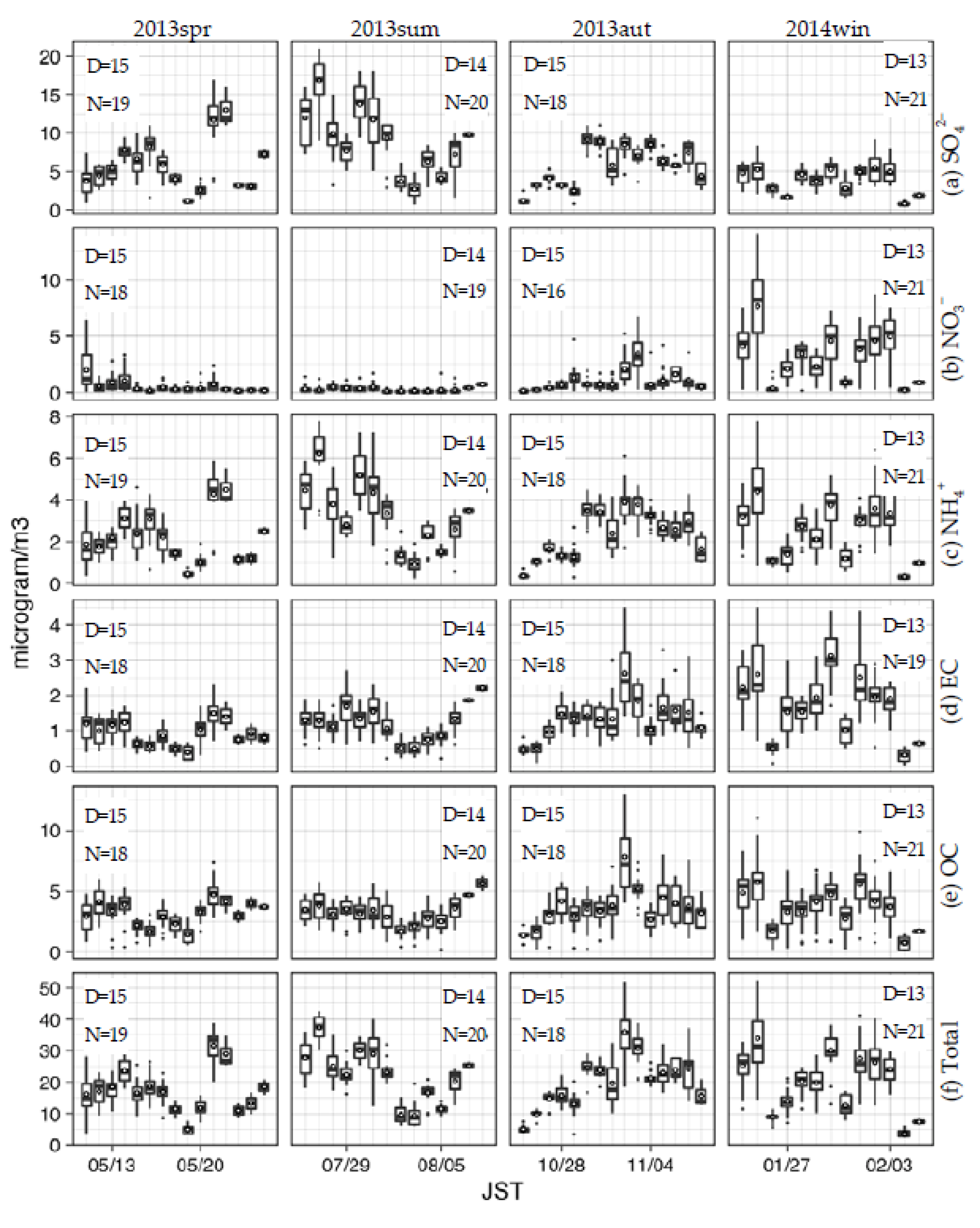
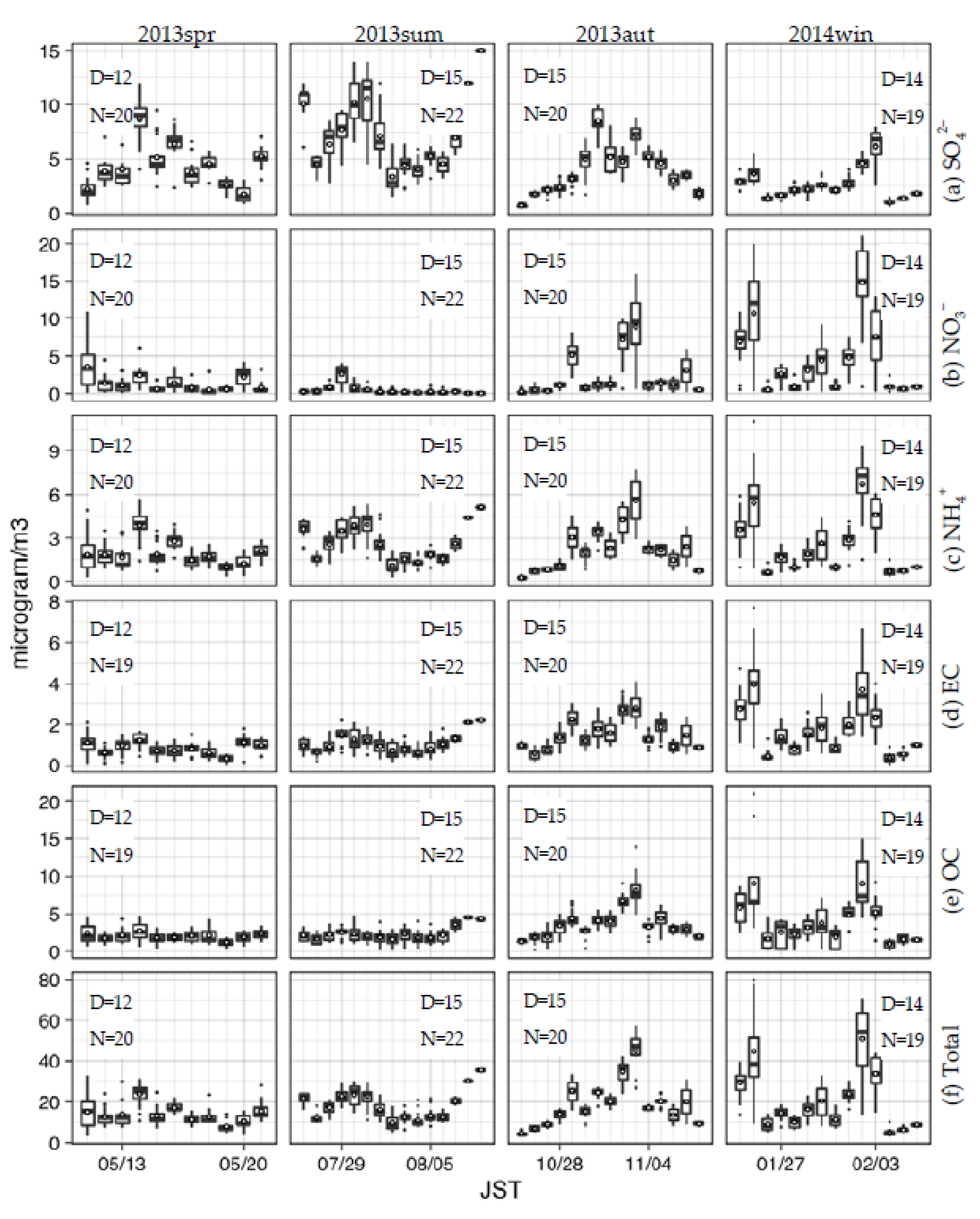
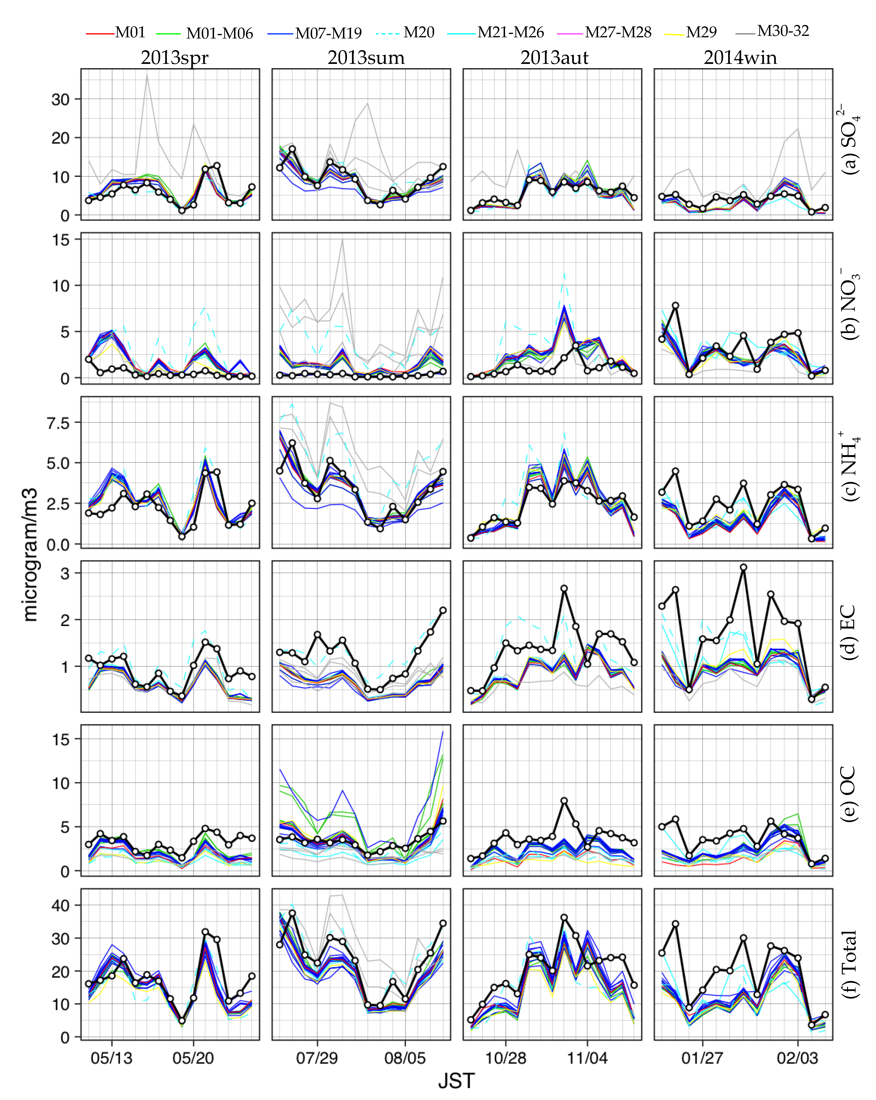
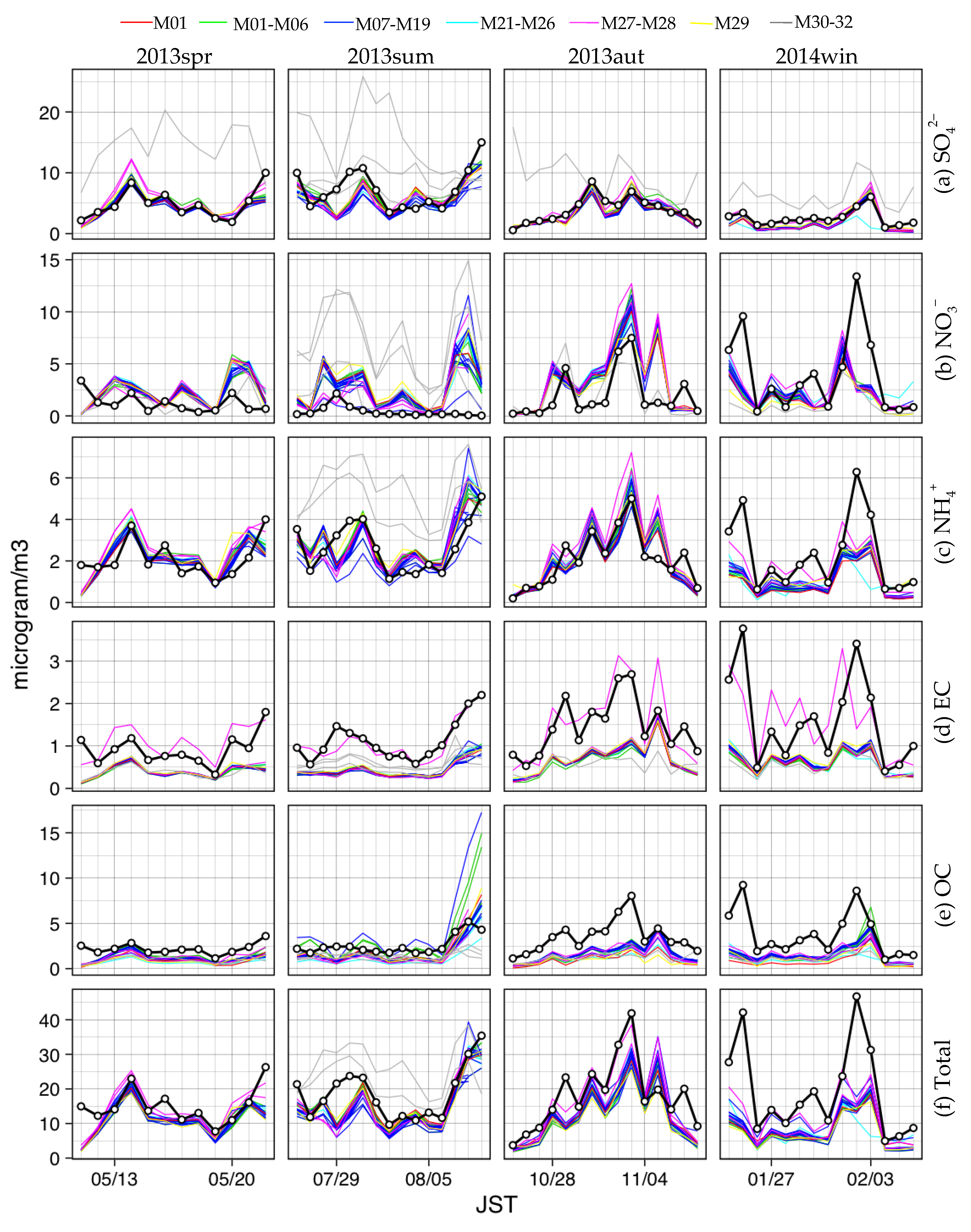
4.2. Simulated Daily Concentrations of PM2.5 Components and Total PM2.5 Mass

Figure 8 and Figure 9 present spatially averages obtained from observed and simulated daily concentrations for PM2.5 components (SO42−, NO3, NH4+, EC, and OC) and total PM2.5 mass for different AAPMSs in d03 and d04, respectively. The seasonal ensemble performances of the participant CTMs at each AAPMS are also summarized as statistics in Table 4 and Table 5 for each domain. The goal and criteria levels for CTM performance statistics, NMB, normalized mean error (NME), and correlation were recommended by Emery et al. [52], and the fractional bias (FB) and fractional error (FE) were recommended by Boylan and Russell [53], which is listed in Table A1. Individual model performance reports of each CTM are shown in Table A2 and Table A3.
With SO42− as a dominant PM2.5 component, most CTMs showed good agreement with daily concentration levels and day-to-day changes in both domains for each season, with the exception of a few model settings. Overall, the ensemble statistics, including the NMB (−0.85, 1.65%), NME (30.34, 29.11), FB (3.66, −13.77%), FE (30.41, 34.28), and correlation (0.74, 0.86), passed the goal level in d03 for summer and autumn. For d04, the NMB (−7.5%), NME (30.34), FB (−13.04%), FE (32.83%), and correlation (0.84) passed the goal level for summer. With the exception of d03 in winter and d04 in summer, the correlation and IoA indicated excellent performance, with maximum values of 0.74–0.88 and 0.79–0.87 for d04 in winter. Most CTMs underestimated the observed SO42− in d04 on 29–30 July, with relatively low values for the correlation (0.36) and IoA (0.52). This result may lead to underestimations of the total PM2.5 mass in connection with the NH4+ concentrations. WRF-Chem (M30, 31) clearly overestimated SO42− concentrations in PM2.5 due to the SO42− mass build-up problem associated with the nucleation calculation in MADE/SORGAM [54]. In addition, the WRF-Chem group employed their own physical parameterizations such as cumulus convection and microphysics for their meteorological simulations. Additional sensitivity simulations for meteorological fields are required to quantitatively evaluate the model inter-differences of SO42− and total PM2.5 mass concentrations owing to the differences in meteorological simulations. We will perform this in the next phase. The largest positive biases were found in M31, with 3.0–9.7 µg/m3 (NMB: 52%–177%) for d03 and 3.8–10.2 µg/m3 (NMB: 131%–240%) for d04. These simulated overestimations were slightly higher for CMAQ Version 4.7.1 (M27 and M28), particularly for d04 in spring. This trend indicates that the updated sulfur chemistries in CMAQ Version 5.0 [35,55,56,57,58] enhanced the performance of this model compared to the previous versions. In winter, CAMx (M29) performed better, with biases of −0.32 µg/m3 (NMB: −7.3%) for d04 and 0.39 µg/m3 (NMB: 3.4%) for d04 under the same emission condition. This result is attributed to an underestimation of SO42− by the dominant participant model, CMAQ, which may be caused by an inadequate aqueous-phase SO42− production by Fe- and Mn-catalyzed O2 oxidation [14].
All participant CTMs overestimated NO3 levels in warmer seasons, with ensemble biases of 1.22–1.55 µg/m3 (NMB: 194%–651%) for d03 and 0.85–1.99 µg/m3 (NMB: 145%–588%) for d04. The largest positive biases were found in summer. Above all, M20, M30, and M31 strongly overestimated elevated NO3levels. Only M11 showed relatively good agreement with observations for d03 in summer, with a minimum bias of 0.12 µg/m3 (NMB: 91%) and improved values for the correlation (0.46) and IoA (0.54). However, M11 also produced low concentrations for SO42− and NH4+. As observed for d04 in autumn, all models exhibited better performance for the daily concentration levels and day-to-day changes in NO3. For example, M30 has a minimum bias of 0.14 µg/m3 (NMB: 11%), which passed the goal NMB level for 24-h NO3. Some deviations in NO3 between observations and the models were attributed to NH4+ and potentially NH4NO3. In winter, most models reproduced day-to-day changes in both domains but tended to underestimate elevated NO3 levels, with ensemble mean biases of −0.89 µg/m3 (NMB: −18.9%) and −2.36 µg/m3 (NMB: −42.8%). A previous model inter-comparison study for the Tokyo metropolitan area, UMICS, concluded that the participant models overestimated NO3 levels in both summer and winter [11,12], although available observations included only one winter and three summer stations. In our validations, most models produced higher NO3 levels in spring and summer, lower NO3 levels in winter, and moderate NO3 levels in autumn, compared with accumulated observation data for d03 and d04. This result is expected to be more accurate than previous reports because a greater number of observations (for 18–22 stations) were included.
As mentioned above, the day-to-day variations in NH4+ were consistent with those of SO42− and NO3. Therefore, most CTMs showed good agreement with daily concentration levels and day-to-day changes in both domains for each season, with the exception of some elevated peaks. Above all, the ensemble performances indicators, FE and FB, were −27.9%–8.9% and 34.3%–41.1%, thus passing the goal level in both domains for all seasons except winter. Notably, the differences among models increased in summer. Two WRF-Chem models (M32, M31) predicted higher NH4+ levels, with biases of 1.96–3.03 µg/m3 (NMB: 84%–130%) and 1.72–2.71 µg/m3 (NMB: 85%–61%) for d03 and d04, respectively. The M20 model, which employed EAGrid for emissions and an original configuration for meteorology, also produced relatively high NH4+ levels in d03, with a bias of 1.68 µg/m3 (NMB: 51%). These overpredictions were likely associated with those of SO42− and NO3 in summer. Meanwhile, relatively larger negative biases were found for M11, at −1.18 µg/m3 (NMB: 35%) for d03 and −0.81 µg/m3 (NMB: 33%) for d04.
The EC levels simulated by most CTMs were considerably lower than the observations in both domains for all season. The model ensemble biases were −0.90 to −0.20 µg/m3 (NMB: −46% to −22%) and −2.77 to −0.39 µg/m3 (NMB: −58% to −40%) for d03 and d04, respectively, with larger values for Tokyo. Both models employing EAGrid2000-JAPAN (M20 (d03) and M27 (d04)) produced higher EC values than other CTMs with different emission settings, and relatively better NMB values were obtained, at −20% to −3% and −35% to 42%, respectively. This trend suggests that the EC emissions of J-STREAM might be underestimated.
The CTMs reproduced some of elevated OC levels in the warmer seasons, but clearly underestimated the observed OC levels for autumn and winter, with model ensemble biases of −1.78 to −0.01 µg/m3 (NMB: −42% to 7%) and −2.77 to −0.81 µg/m3 (NMB: −59% to −39%) for d03 and d04, respectively, which are similar to the EC values. Additionally, as observed for the EC, the negative biases of OC for the Tokyo area were larger than those for western Japan. However, the negative biases of all participant CTMs have been clearly moderated compared with the UMICS cases [11,12]. Among the models, M02, M03, and M11 predicted relatively higher OC levels and overestimated the summer OC concentrations. Full-domain nesting simulations were performed via M02 and M03 using a relatively recent CMAQ model (Version 5.1), which includes updates for some chemical and aerosol mechanisms, such as POA aging, SOA mass yields with new pathways from isoprene, alkanes, and PAHs, and SOA formation reactions in the aqueous-phase chemistry. Continual nesting simulations for the Asian scale (d01) performed by CMAQ Version 5.1 exhibited higher regional-scale OC levels, leading to higher OC levels in urban areas in Japan compared with previous versions. Thus, an empirical SOA yield model can predict the same OC concentration level as the VBS model M11. It should be noted that effect of the updated SOA yield mechanisms was not clear at the urban scale when using CMAQ Version 5.1 or higher (e.g., M01, M04–05). Additionally, to evaluate simulated OC concentrations, more observational data are needed.
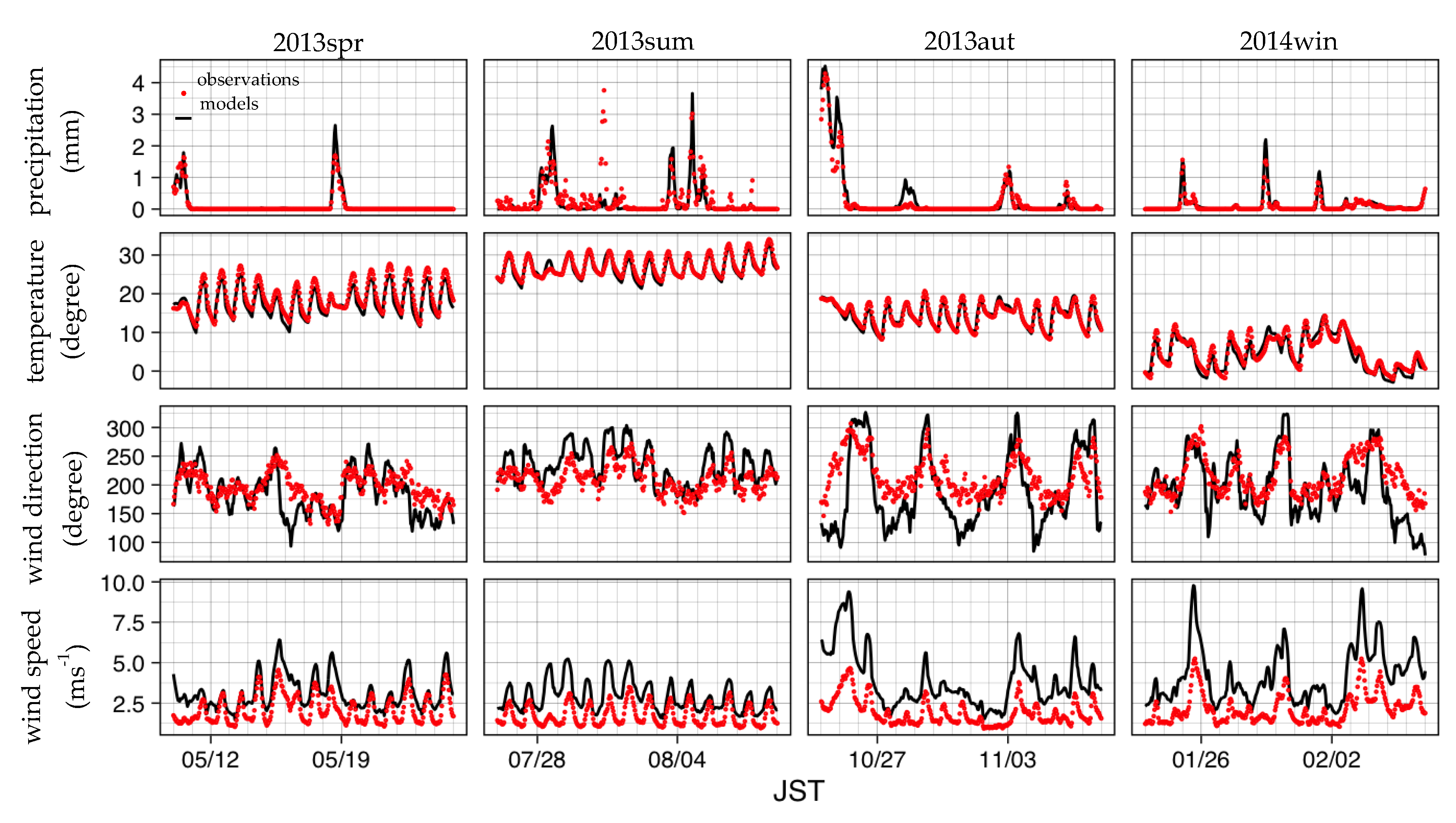
Overall, most CTMs showed good agreement with observed concentration levels of total PM2.5 mass in both domains for each season. These results are likely associated with the reproducibility of some dominant components, e.g., SO42− and NH4+. Moreover, CTMs tended to fail at reproducing some heavily polluted situations and underestimated the considerably high PM2.5 concentrations (approximately 40–50 µg/m3). A considerable underestimation (≈30 µg/m3) of total PM2.5 associated with PM2.5 components, except for SO42−, was observed for d04 in the winter season, 25 January and 2 February; during that time, the nighttime simulated surface temperature was clearly lower than that in the observations (Figure 3). This implies that the simulated higher surface temperature compared with that in the observations formed weaker atmospheric stability, which produced weaker accumulations of particulate pollutants at nighttime, especially during colder seasons. The model ensemble biases were −8.66 to −0.99 µg/m3 (NMB: −43% to −5%) for d03 and −2.91 to −11.98 µg/m3 (NMB: −55% to −19%) for d04. The largest negative biases are found in winter due to underestimations of NH4NO3, particularly for d04. M31 and M32 tended to overpredict the total PM2.5 due to overestimates of inorganic compounds. Of the model ensemble statistics for d03, the NMB (−5%, 13%) NME (22%, 26%), FB (−9%, −17%), FE (26%, 29%), and correlation (0.81, 0.78) passed the goal level for 24-h total PM2.5 mass in spring and summer, respectively. In addition, the majority of the other statistical indicators passed the criteria levels as well.

5. Summery

A model inter-comparison of secondary pollutant simulations over urban areas in Japan, J-STREAM Phase I, was performed, in which a total of 32 simulations were conducted by combining CMAQ, CAMx, and WRF-Chem.
Simulated hourly concentrations of the primary pollutants NO and NO2, which are precursors of PM2.5, generally showed good agreement with the observed concentrations, at the same level as the MICS case. However, some differences between observations and simulations and CTMs may be considered to be caused by the differences in meteorological conditions and NOx chemistries of each CTM. Furthermore, most of the CTMs using the same input emissions tended to overestimate SO2 concentrations, although the models showed good performance for PM2.5 SO42−. The different emission inventory, EAGrid produced better results for SO2; therefore, it appears that the emission input can be improved. However, it was likely to be unrealistic that just the modifications of the emissions could fully resolve the overestimation of SO2.
Simulated concentrations of PM2.5 and its components were evaluated via a comparison with daily observed concentrations by using the filter pack method at selected AAPMSs for a period of at least two weeks for each season in this project. In general, most of the models showed good agreement with the observed concentration of total PM2.5 mass for each season, within goal or criteria levels of model ensemble statistics especially in warmer seasons. This agreement was associated with the reproducibility of some of dominant particulates.
Among individual PM2.5 components, most model results for SO42− and NH4+ showed good agreement with daily concentration levels and day-to-day variations, with good model ensemble statistics, particularly for the warmer seasons. However, for SO42−, a problem in the WRF-Chem model and novel, improved mechanisms for SO42− formation in most CTMs were found through this model inter-comparison. Additionally, we found that the differences in the Asian scale precipitation patterns between precipitation parametrizations affected the simulated water-soluble PM2.5 concentrations. Additional improvements for SO42− were expected, particularly for the winter [11]. All participant models showed a strong tendency to overestimate NO3 in warmer seasons, with the model ensemble NMB reaching 651%. However, in winter, most of the models reproduced the day-to-day variations, with underestimations for elevated NO3 levels. These tendencies differed from a previous model inter-comparison, UMICS, which concluded that the participant models overestimated NO3 levels in both summer and winter [11,12]. This difference between two model inter-comparison studies is attributed to variations in the number of observations applied for verification. Thus, a sufficient amount of observation data on PM2.5 components is needed to evaluate and improve CTMs. The EC levels simulated by most models were considerably lower than the observed levels for all seasons; however, some models employing EAGrid emissions produced higher EC levels than the other models. The models reproduced concentrations for some elevated OC values in the warmer seasons, but clearly underestimated the OC levels in autumn and winter. In addition, some models employing the VBS model and the newly updated SOA yield mechanisms produced higher OC levels and even overestimated the observed OC concentration in some cases.
This study has identified some effective approaches for improving PM2.5 simulations for urban areas in Japan based on a model inter-comparison. First, improvements in emissions are expected to increase the reproducibility of primary pollutants that are precursors of PM2.5 and EC concentrations. For SO42−, NO3, and OC, additional formation pathways can help to reduce underestimations. The recent model updates (e.g., CMAQ Version 5.3) improved the chemical pathways and are expected to simulate the secondary PM2.5 components well. Simulated meteorological fields will be important for the Asian scale PM2.5 concentration levels and the elevated PM2.5 concentrations during the days with high amounts of pollution. In addition, special attention is needed for misjudgments in these models. Finally, additional accumulated observations are needed to evaluate the simulated concentrations. Future studies will include these modifications to realize reference air quality modeling in the next stages of J-STREAM.

Author Contributions

K.Y. managed the model inter-comparison (J-STREAM), prepared the initial, boundary, and meteorological inputs, and wrote this article. S.C. is the leader of J-STREAM project and prepared emission inputs. S.I. and H.H. are core members of J-STREAM in charge of inorganic aerosols. T.S. is a core member of J-STREAM in charge of photochemical gases. M.S., M.T., T.M. (Tazuko Morikawa), I.K., Y.M. (Yukako Miya), H.K., Y.M. (Yu Morino), K.K., T.N., H.S., K.U., and Y.F. are participants who conducted the model simulations. T.H. and T.M. (Takeshi Misaki) analyzed the submitted data. K.S. is in charge of global simulations. All authors have read and agreed to the published version of the manuscript.

Funding

This research was funded by the Environment Research and Technology Development Fund (5-1601) of the Environmental Restoration and Conservation Agency, JSPS KAKENHI Grant Number 18H03369, and the Collaborative Research Program of Research Institute for Applied Mechanics, Kyushu University.

Acknowledgments

This project was supported by the Environment Research and Technology Development Fund (5-1601) of the Environmental Restoration and Conservation Agency. This work was also partially supported by JSPS KAKENHI Grant Number 18H03369. Monitoring data of APMSs were obtained from National Institute for Environmental Studies. This work was supported in part by the Collaborative Research Program of Research Institute for Applied Mechanics, Kyushu University.

Conflicts of Interest

The authors declare no conflict of interest.

Appendix A

Table A1. Recommended benchmarks for photochemical model performance statistics [52,53].
NMBNMErFBFE
SpeciesGoalCriteriaGoalCriteriaGoalCriteriaGoalCriteriaGoalCriteria
24-h PM2.5, SO42−, NH4+<±10%<±30%<35%<50%>0.70>0.40<±30%<±60%<±60%<±75%
24-h NO3<±15%<±65%<65%<115%NoneNone
24-h OC<±15%<±50%<45%<65%NoneNone
24-h EC<±20%<±40%<50%<75%NoneNone
Table A2. Individual model performance (IoA) for d03.
ID2013Spr2013Sum
SO42−NO3NH4+ECOCTOTALSO42−NO3NH4+ECOCTOTAL
M010.820.320.740.710.620.860.840.190.800.600.620.83
M020.800.350.740.730.760.870.840.240.810.620.390.84
M030.810.340.750.740.700.880.850.230.820.590.340.83
M040.810.360.740.710.730.860.830.230.800.610.640.83
M050.800.330.720.720.740.860.840.220.800.620.630.83
M060.850.350.760.690.710.850.820.250.800.570.650.78
M070.820.350.750.710.700.850.870.230.830.650.610.86
M080.820.330.740.730.720.860.860.200.810.630.640.83
M090.830.330.750.730.720.860.840.200.810.630.640.82
M10 0.840.200.810.620.640.82
M11 0.690.430.660.540.300.76
M120.800.320.720.730.730.860.860.190.810.620.630.84
M130.810.340.700.730.620.860.850.190.800.630.640.83
M140.830.330.740.720.720.850.860.210.820.630.640.79
M150.830.330.740.720.710.870.860.210.820.620.640.84
M16 0.850.210.810.620.640.82
M17 0.850.200.810.620.640.83
M18 0.850.200.810.620.640.83
M19 0.850.200.800.620.630.83
M200.84 0.20 0.690.700.550.810.850.070.710.630.590.84
M210.82 0.32 0.730.720.720.850.850.190.810.630.640.83
M220.82 0.32 0.740.730.590.860.850.210.810.620.620.82
M230.84 0.36 0.760.710.700.870.860.220.820.620.640.83
M240.84 0.36 0.760.710.700.870.860.220.820.620.640.83
M260.83 0.37 0.730.710.500.870.860.210.810.620.500.81
M290.81 0.42 0.750.710.540.800.860.220.810.620.590.81
M300.27 0.32 0.660.50 0.360.220.570.540.420.69
M31 0.680.060.700.690.540.83
M32 0.840.07 0.680.52
ID2013Aut2013Win
SO42−NO3NH4+ECOCTOTALSO42−NO3NH4+ECOCTOTAL
M010.910.300.850.850.460.790.690.600.690.550.450.61
M020.890.350.830.830.560.770.700.570.740.570.530.63
M030.840.380.800.800.500.770.700.570.760.570.470.63
M040.900.340.850.850.530.790.690.570.710.550.530.64
M050.900.320.840.840.540.800.690.580.720.560.530.65
M060.900.320.850.850.510.770.700.580.680.550.530.62
M070.910.290.840.840.520.800.690.510.690.520.510.64
M080.900.300.830.830.540.800.710.630.750.580.550.67
M090.900.300.830.830.540.800.690.610.740.580.550.67
M10
M11 0.420.260.390.440.310.40
M120.890.290.800.800.550.810.710.600.760.580.560.69
M130.860.330.790.790.490.810.710.580.770.580.530.67
M140.910.310.830.830.550.760.700.610.740.580.540.62
M150.910.300.840.840.540.800.700.610.740.570.540.66
M16
M17
M18
M19
M200.880.190.700.700.490.740.710.560.780.650.500.67
M210.910.290.830.830.560.800.680.570.690.630.600.65
M220.900.300.830.830.480.800.460.030.340.440.350.35
M230.900.330.850.850.530.790.690.600.710.570.540.64
M240.900.340.850.850.530.790.690.600.710.570.540.64
M260.900.330.840.840.440.790.700.580.730.570.490.64
M290.910.320.830.830.440.740.700.620.720.600.500.61
M300.300.36 0.44 0.270.52 0.530.48
M31 0.720.190.310.410.330.46
M32 0.420.110.310.400.320.36
M31
M32
Table A3. Individual model performance (IoA) for d04.
ID2013Spr2013Sum
SO42−NO3NH4+ECOCTOTALSO42−NO3NH4+ECOCTOTAL
M010.860.340.710.500.480.670.590.330.710.440.380.64
M020.880.380.760.520.530.690.590.340.710.440.290.63
M030.860.390.740.510.530.700.610.380.700.430.270.62
M040.870.350.720.510.510.690.630.320.730.440.410.67
M050.870.350.720.510.500.680.620.330.720.440.410.66
M060.860.360.710.500.480.640.560.400.680.430.410.59
M070.860.380.720.510.500.700.620.370.710.430.380.61
M080.870.350.710.510.510.670.560.360.660.440.390.60
M090.870.370.730.510.510.670.560.370.660.440.390.60
M10 0.570.350.670.440.410.61
M11 0.520.540.560.440.280.52
M120.880.350.710.510.520.680.560.340.660.440.390.60
M130.880.360.700.510.470.670.550.340.680.440.390.62
M140.880.340.730.510.510.670.560.340.660.440.400.58
M150.880.340.730.510.510.700.550.340.660.440.390.59
M16 0.570.340.670.440.410.61
M17 0.570.350.670.440.410.61
M18 0.580.330.680.440.410.62
M19 0.570.330.690.440.400.63
M210.880.340.720.510.500.680.570.350.670.440.410.61
M220.880.340.720.510.450.680.570.350.670.440.400.62
M230.880.360.740.510.510.700.580.330.690.430.400.62
M240.880.360.750.510.510.700.580.340.690.430.400.62
M250.890.360.730.510.460.710.550.370.690.420.380.61
M260.880.350.720.510.420.690.570.320.700.430.360.63
M270.790.380.670.540.530.680.600.410.710.560.440.63
M280.820.340.660.520.470.680.580.360.700.430.370.59
M290.860.360.660.520.430.640.590.310.730.460.420.67
M300.270.31 0.470.46 0.320.37 0.430.39
M31 0.430.150.400.550.520.52
M32 0.650.160.550.530.540.70
ID2013Aut2013Win
SO42−NO3NH4+ECOCTOTALSO42−NO3NH4+ECOCTOTAL
M010.880.590.820.560.760.760.860.570.640.510.460.56
M020.910.580.800.570.760.760.880.560.670.520.500.57
M030.900.590.780.540.760.760.880.580.680.500.470.57
M040.890.580.800.560.770.770.870.550.650.510.490.58
M050.890.580.800.570.790.790.880.570.660.520.490.58
M060.850.580.800.560.730.730.860.560.630.510.490.57
M070.880.540.770.570.770.770.900.560.670.520.500.63
M080.880.550.780.570.760.760.880.570.660.520.500.59
M090.880.550.780.570.750.750.870.560.660.520.500.59
M10
M11
M120.900.540.770.570.770.770.890.570.680.520.500.60
M130.910.570.770.560.770.770.890.550.690.520.470.59
M140.890.550.780.570.730.730.870.580.670.530.500.57
M150.880.560.790.570.760.760.870.580.670.530.500.59
M16
M17
M18
M19
M210.880.550.780.570.760.760.520.530.540.520.480.53
M220.880.550.780.570.760.760.870.570.660.520.470.59
M230.880.570.790.560.750.750.870.570.660.510.490.58
M240.880.570.790.560.750.750.870.560.650.510.490.58
M250.910.540.760.580.790.790.870.560.680.520.470.59
M260.890.570.790.560.760.760.870.550.670.510.460.58
M270.910.550.720.720.810.810.880.530.700.620.490.64
M280.920.550.760.580.790.790.880.530.680.510.470.60
M290.920.560.790.580.740.740.910.570.650.540.490.56
M300.200.52 0.50 0.460.53 0.490.46
M31
M32

References

  1. World Health Organization. Ambient Air Pollution: A Global Assessment of Exposure and Burden of Disease. Available online: https://www.who.int/phe/publications/air-pollution-global-assessment/en/ (accessed on 14 January 2020).
  2. Fiore, A.M.; Naik, V.; Leibensperger, E.M. Air quality and climate connections. J. Air Waste Manag. Assoc. 2015, 65, 645–685. [Google Scholar] [CrossRef] [PubMed]
  3. Zhang, Q.; Zheng, Y.; Tong, D.; Shao, M.; Wang, S.; Zhang, Y.; Xu, X.; Wang, J.; He, H.; Liu, W.; et al. Drivers of improved PM2.5 air quality in China from 2013 to 2017. Proc. Natl. Acad. Sci. USA 2019, 116, 24463–24469. [Google Scholar] [CrossRef] [PubMed] [Green Version]
  4. Ministry of the Environment. Available online: http://www.env.go.jp/air/osen/monitoring.html (accessed on 14 January 2020).
  5. Chatani, S.; Yamaji, K.; Sakurai, T.; Itahashi, S.; Shimadera, H.; Kitayama, K.; Hayami, H. Overview of Model Inter-Comparison in Japan’s Study for Reference Air Quality Modeling (J-STREAM). Atmosphere 2018, 9, 19. [Google Scholar] [CrossRef] [Green Version]
  6. Carmichael, G.; Sakurai, T.; Streets, D.; Hozumi, Y.; Ueda, H.; Park, S.; Fung, C.; Han, Z.; Kajino, M.; Engardt, M. MICS-Asia II: The model intercomparison study for Asia Phase II methodology and overview of findings. Atmos. Environ. 2008, 42, 3468–3490. [Google Scholar] [CrossRef]
  7. Carmichael, G.R.; Calori, G.; Hayami, H.; Uno, I.; Cho, S.Y.; Engardt, M.; Kim, S.-B.; Ichikawa, Y.; Ikeda, Y.; Woo, J.H.; et al. model intercomparison of long-range transport and sulfur deposition in East Asia. Atmos. Environ. 2002, 36, 175–199. [Google Scholar] [CrossRef]
  8. Chen, L.; Gao, Y.; Zhang, M.; Fu, J.-S.; Zhu, J.; Liao, H.; Li, J.; Huang, K.; Ge, B.; Wang, X.; et al. MICS-Asia III: Multi-model comparison and evaluation of aerosol over East Asia. Atmos. Chem. Phys. Discuss. 2019, 2019, 1–54. [Google Scholar] [CrossRef] [Green Version]
  9. Li, J.; Nagashima, T.; Kong, L.; Ge, B.; Yamaji, K.; Fu, J.-S.; Wang, X.; Fan, Q.; Itahashi, S.; Lee, H.J.; et al. Model evaluation and inter-comparison of surface-level ozone and relevant species in East Asia in the context of MICS-Asia phase III Part I: Overview. Atmos. Chem. Phys. Discuss. 2019, 2019, 1–56. [Google Scholar] [CrossRef]
  10. Chatani, S.; Morino, Y.; Shimadera, H.; Hayami, H.; Mori, Y.; Sasaki, K.; Kajino, M.; Yokoi, T.; Morikawa, T.; Ohara, T. Multi-Model Analyses of Dominant Factors Influencing Elemental Carbon in Tokyo Metropolitan Area of Japan. Aerosol Air Qual. Res. 2014, 14, 396–405. [Google Scholar] [CrossRef] [Green Version]
  11. Shimadera, H.; Hayami, H.; Chatani, S.; Morino, Y.; Mori, Y.; Morikawa, T.; Yamaji, K.; Ohara, T. Sensitivity analyses of factors influencing CMAQ performance for fine particulate nitrate. J. Air Waste Manag. Assoc. 2017, 64, 374–387. [Google Scholar] [CrossRef] [Green Version]
  12. Shimadera, H.; Hayami, H.; Chatani, S.; Morikawa, T.; Morino, Y.; Mori, Y.; Yamaji, K.; Nakatsuka, S.; Ohara, T. Urban Air Quality Model Inter-Comparison Study (UMICS) for Improvement of PM2.5 Simulation in Greater Tokyo Area of Japan. Asian J. Atmos. Environ. 2018, 12, 139–152. [Google Scholar] [CrossRef]
  13. Chatani, S.; Yamaji, K.; Itahashi, S.; Saito, M.; Takigawa, M.; Morikawa, T.; Kanda, I.; Miya, Y.; Komatsu, H.; Sakurai, T.; et al. Identifying key factors influencing model performance on ground-level ozone over urban areas in Japan through model inter-comparisons. Atmos. Environ. 2020, 223. [Google Scholar] [CrossRef]
  14. Itahashi, S.; Yamaji, K.; Chatani, S.; Hayami, H. Refinement of Modeled Aqueous-Phase Sulfate Production via the Fe- and Mn-Catalyzed Oxidation Pathway. Atmosphere 2018, 9, 132. [Google Scholar] [CrossRef] [Green Version]
  15. Skamarock, W.C.; Klemp, J.B.; Dudhia, J.; Gill, D.O.; Barker, D.M.; Duda, M.G.; Huang, X.Y.; Wang, W.; Powers, J.G. A Description of the Advanced Research WRF Version 3; University Corporation for Atmospheric Research: Boulder, CO, USA, 2008. [Google Scholar]
  16. NCEP FNL Operational Model Global Tropospheric Analyses, continuing from July 1999. Research Data Archive at the National Center for Atmospheric Research; Computational and Information Systems Laboratory: Boulder, CO, USA, 2000. [Google Scholar]
  17. Gemmill, W.; Katz, B.; Li, X. Daily Real-Time, Global Sea Surface Temperature a High-Resolution Analysis: RTG_SST_HR, NOAA/NWS/NCEP/EMC/MMAB, Science Application International Corporation, and Joint Center for Satellite Data Assimilation Technical Note Nr. NOAA/NWS/NCEP/MMAB Off. Note 2007, 260, 1–39. [Google Scholar]
  18. Hong, S.Y.; Dudhia, J.; Chen, S.H. A revised approach to ice microphysical processes for the bulk parameterization of clouds and precipitation. Mon. Weather Rev. 2004, 132, 103–120. [Google Scholar] [CrossRef]
  19. Mlawer, E.J.; Taubman, S.J.; Brown, P.D.; Iacono, M.J.; Clough, S.A. Radiative transfer for inhomogeneous atmospheres: RRTM, a validated correlated-k model for the longwave. J. Geophys Res. Atmos 1997, 102, 16663–16682. [Google Scholar] [CrossRef] [Green Version]
  20. Dudhia, J. Numerical Study of Convection Observed during the Winter Monsoon Experiment Using a Mesoscale Two-Dimensional Model. J. Atmos. Sci. 1989, 46, 3077–3107. [Google Scholar] [CrossRef]
  21. Chen, F.; Dudhia, J. Coupling an advanced land surface-hydrology model with the Penn State-NCAR MM5 modeling system. Part I: Model implementation and sensitivity. Mon. Weather Rev. 2001, 129, 569–585. [Google Scholar] [CrossRef] [Green Version]
  22. Nakanishi, M.; Niino, H. An improved mellor-yamada level-3 model: Its numerical stability and application to a regional prediction of advection fog. Bound. Layer Meteorol. 2006, 119, 397–407. [Google Scholar] [CrossRef]
  23. Kain, J.-S. The Kain-Fritsch convective parameterization: An update. J. Appl. Meteorol. 2004, 43, 170–181. [Google Scholar] [CrossRef] [Green Version]
  24. Byun, D.; Schere, K.L. Review of the Governing Equations, Computational Algorithms, and Other Components of the Models-3 Community Multiscale Air Quality(CMAQ) Modeling System. Appl. Mech. Rev. 2006, 59, 51–77. [Google Scholar] [CrossRef]
  25. Ramboll Environment and Health. User’s Guide Comprehensive Air Quality Model with Extensions. Available online: http://www.camx.com/files/camxusersguide_v6-50.pdf (accessed on 14 January 2020).
  26. Grell, G.A.; Peckham, S.E.; Schmitz, R.; McKeen, S.A.; Frost, G.; Skamarock, W.C.; Eder, B. Fully coupled “online” chemistry within the WRF model. Atmos. Environ. 2005, 39, 6957–6975. [Google Scholar] [CrossRef]
  27. Carter, W.P.L. Documentation of the SAPRC-99 chemical mechanism for VOC reactivity assessment. Contract 2000, 92, 95–308. [Google Scholar]
  28. Carter, W.P.L. Development of the SAPRC-07 chemical mechanism. Atmos. Environ. 2010, 44, 5324–5335. [Google Scholar] [CrossRef]
  29. Whitten, G.Z.; Heo, G.; Kimura, Y.; McDonald-Buller, E.; Allen, D.T.; Carter, W.P.L.; Yarwood, G. A new condensed toluene mechanism for Carbon Bond CB05-TU. Atmos. Environ. 2010, 44, 5346–5355. [Google Scholar] [CrossRef]
  30. Goliff, W.S.; Stockwell, W.R.; Lawson, C.V. The regional atmospheric chemistry mechanism, version 2. Atmos. Environ. 2013, 68, 174–185. [Google Scholar] [CrossRef]
  31. Binkowski, F.S. Models-3 Community Multiscale Air Quality (CMAQ) model aerosol component 1. Model description. J. Geophys. Res. 2003, 108. [Google Scholar] [CrossRef]
  32. Koo, B.; Knipping, E.; Yarwood, G. 1.5-Dimensional volatility basis set approach for modeling organic aerosol in CAMx and CMAQ. Atmos. Environ. 2014, 95, 158–164. [Google Scholar] [CrossRef]
  33. Nenes, A.; Pandis, S.N.; Pilinis, C. ISORROPIA: A new thermodynamic equilibrium model for multiphase multicomponent inorganic aerosols. Aquat. Geochem. 1998, 4, 123–152. [Google Scholar] [CrossRef]
  34. Nenes, A.; Pandis, S.N.; Pilinis, C. Continued development and testing of a new thermodynamic aerosol module for urban and regional air quality models. Atmos. Environ. 1999, 33, 1553–1560. [Google Scholar] [CrossRef]
  35. Fountoukis, C.; Nenes, A. ISORROPIA II: A computationally efficient thermodynamic equilibrium model for K+-Ca2+-Mg2+-Nh4+-Na+-SO42−-NO3-Cl-H2O aerosols. Atmos. Chem. Phys. 2007, 7, 4639–4659. [Google Scholar] [CrossRef] [Green Version]
  36. Carlton, A.G.; Bhave, P.V.; Napelenok, S.L.; Edney, E.D.; Sarwar, G.; Pinder, R.W.; Pouliot, G.A.; Houyoux, M. Model Representation of Secondary Organic Aerosol in CMAQv4.7. Environ. Sci. Technol. 2010, 44, 8553–8560. [Google Scholar] [CrossRef]
  37. Itahashi, S.; Yamaji, K.; Chatani, S.; Hisatsune, K.; Saito, S.; Hayami, H. Model Performance Differences in Sulfate Aerosol in Winter over Japan Based on Regional Chemical Transport Models of CMAQ and CAMx. Atmosphere 2018, 9, 488. [Google Scholar] [CrossRef] [Green Version]
  38. Ackermann, I.J.; Hass, H.; Memmesheimer, M.; Ebel, A.; Binkowski, F.S.; Shankar, U. Modal aerosol dynamics model for Europe: Development and first applications. Atmos. Environ. 1998, 32, 2981–2999. [Google Scholar] [CrossRef]
  39. Schell, B.; Ackermann, I.J.; Hass, H.; Binkowski, F.S.; Ebel, A. Modeling the formation of secondary organic aerosol within a comprehensive air quality model system. J. Geophys. Res. Atmos 2001, 106, 28275–28293. [Google Scholar] [CrossRef]
  40. Sudo, K.; Takahashi, M.; Kurokawa, J.; Akimoto, H. CHASER: A global chemical model of the troposphere - 1. Model description. J. Geophys. Res. Atmos. 2002, 107. [Google Scholar] [CrossRef] [Green Version]
  41. Huang, M.; Carmichael, G.R.; Pierce, R.B.; Jo, D.S.; Park, R.J.; Flemming, J.; Emmons, L.K.; Bowman, K.W.; Henze, D.K.; Davila, Y.; et al. Impact of intercontinental pollution transport on North American ozone air pollution: An HTAP phase 2 multi-model study. Atmos. Chem. Phys. 2017, 17, 5721–5750. [Google Scholar] [CrossRef] [PubMed] [Green Version]
  42. Janssens-Maenhout, G.; Crippa, M.; Guizzardi, D.; Dentener, F.; Muntean, M.; Pouliot, G.; Keating, T.; Zhang, Q.; Kurokawa, J.; Wankmuller, R.; et al. HTAP_v2.2: A mosaic of regional and global emission grid maps for 2008 and 2010 to study hemispheric transport of air pollution. Atmos. Chem. Phys. 2015, 15, 11411–11432. [Google Scholar] [CrossRef] [Green Version]
  43. van der Werf, G.R.; Randerson, J.T.; Giglio, L.; van Leeuwen, T.T.; Chen, Y.; Rogers, B.M.; Mu, M.; van Marle, M.J.E.; Morton, D.C.; Collatz, G.J.; et al. Global fire emissions estimates during 1997–2015. Earth Syst. Sci. Data Discuss. 2017, 2017, 1–43. [Google Scholar] [CrossRef]
  44. Chatani, S.; Morikawa, T.; Nakatsuka, S.; Matsunaga, S.; Minoura, H. Development of a framework for a high-resolution, three-dimensional regional air quality simulation and its application to predicting future air quality over Japan. Atmos. Environ. 2011, 45, 1383–1393. [Google Scholar] [CrossRef]
  45. Diehl, T.; Heil, A.; Chin, M.; Pan, X.; Streets, D.; Schultz, M.; Kinne, S. Anthropogenic, biomass burning, and volcanic emissions of black carbon, organic carbon, and SO2 from 1980 to 2010 for hindcast model experiments. Atmos. Chem. Phys. Discuss. 2012, 2012, 24895–24954. [Google Scholar] [CrossRef] [Green Version]
  46. Japan Meteorological Agency. Available online: http://www.data.jma.go.jp/svd/vois/data/tokyo/volcano.html (accessed on 14 January 2020).
  47. Guenther, A.B.; Jiang, X.; Heald, C.L.; Sakulyanontvittaya, T.; Duhl, T.; Emmons, L.K.; Wang, X. The Model of Emissions of Gases and Aerosols from Nature version 2.1 (MEGAN2.1): An extended and updated framework for modeling biogenic emissions. Geosci. Model Dev. 2012, 5, 1471–1492. [Google Scholar] [CrossRef] [Green Version]
  48. Tetsuo Fukui, K.K. Tsuyoshi Baba, Akiyoshi Kannari. Updating EAGrid2000-Japan emissions inventory based on the recent emission trends. J. Jpn. Soc. Atmos. Environ. 2014, 49, 9. [Google Scholar]
  49. Kannari, A.; Tonooka, Y.; Baba, T.; Murano, K. Development of multiple-species 1km×1km resolution hourly basis emissions inventory for Japan. Atmos. Environ. 2007, 41, 3428–3439. [Google Scholar] [CrossRef]
  50. Zhang, Q.; Streets, D.G.; Carmichael, G.R.; He, K.B.; Huo, H.; Kannari, A.; Klimont, Z.; Park, I.S.; Reddy, S.; Fu, J.-S.; et al. Asian emissions in 2006 for the NASA INTEX-B mission. Atmos. Chem. Phys. 2009, 9, 5131–5153. [Google Scholar] [CrossRef] [Green Version]
  51. Emmons, L.K.; Walters, S.; Hess, P.G.; Lamarque, J.F.; Pfister, G.G.; Fillmore, D.; Granier, C.; Guenther, A.; Kinnison, D.; Laepple, T.; et al. Description and evaluation of the Model for Ozone and Related chemical Tracers, version 4 (MOZART-4). Geosci. Model Dev. 2010, 3, 43–67. [Google Scholar] [CrossRef] [Green Version]
  52. Emery, C.; Liu, Z.; Russell, A.G.; Odman, M.T.; Yarwood, G.; Kumar, N. Recommendations on statistics and benchmarks to assess photochemical model performance. J. Air Waste Manag. Assoc. 2017, 67, 582–598. [Google Scholar] [CrossRef] [PubMed] [Green Version]
  53. Boylan, J.W.; Russell, A.G. PM and light extinction model performance metrics, goals, and criteria for three-dimensional air quality models. Atmos. Environ. 2006, 40, 4946–4959. [Google Scholar] [CrossRef]
  54. Zhang, Y.; He, J.; Zhu, S.; Gantt, B. Sensitivity of simulated chemical concentrations and aerosol-meteorology interactions to aerosol treatments and biogenic organic emissions in WRF/Chem. J. Geophys. Res. Atmos. 2016, 121, 6014–6048. [Google Scholar] [CrossRef]
  55. Alexander, B.; Park, R.J.; Jacob, D.J.; Gong, S. Transition metal-catalyzed oxidation of atmospheric sulfur: Global implications for the sulfur budget. J. Geophys. Res. 2009, 114. [Google Scholar] [CrossRef] [Green Version]
  56. Jacobson, M.Z. Development and application of a new air pollution modeling system.2. Aerosol module structure and design. Atmos. Environ. 1997, 31, 131–144. [Google Scholar] [CrossRef]
  57. Martin, L.R.; Good, T.W. Catalyzed Oxidation of Sulfur-Dioxide in Solution-The Iron-Manganese Synergism. Atmos. Environ. Part A Gen. Top. 1991, 25, 2395–2399. [Google Scholar] [CrossRef]
  58. Siefert, R.L.; Johansen, A.M.; Hoffmann, M.R.; Pehkonen, S.O. Measurements of trace metal (Fe, Cu, Mn, Cr) oxidation states in fog and stratus clouds. J. Air Waste Manag. Assoc. 1998, 48, 128–143. [Google Scholar] [CrossRef] [PubMed]
Figure 1. Finest model domains for J-STREAM, d03 (a) and d04 (b). d03 covers major city clusters located in western Japan including Osaka, Kobe, Kyoto, and Nagoya. d04 covers the Tokyo metropolitan area. The red circles indicate the locations of ambient air pollution monitoring stations (AAPMSs). The black circles indicate the locations of the meteorological observation stations of the Japan Meteorological Agency (JMA).
Atmosphere 11 00222 g001
Figure 2. Spatially averaged precipitation, temperature, wind direction, and wind speed over four seasons. These results are based on hourly observed values and simulated at all JMA stations for d03.
Atmosphere 11 00222 g002
Figure 3. Spatially averaged precipitation, temperature, wind direction, and wind speed over the four seasons. These results are based on hourly observed values and simulated at all JMA stations for d04.
Atmosphere 11 00222 g003
Figure 4. Box-plots of observed daily concentrations of total particulate matter with a diameter of 2.5 µm or less (PM2.5) and its components: (a) sulfates (SO42−), (b) nitrates (NO3), (c) ammonium (NH4+), (d) elemental carbon (EC), (e) organic carbon (OC), and (f) total PM2.5 mass, at AAPMSs within d03 for the four seasons. The open circles indicate spatially averages obtained from daily concentrations observed at AAPMSs within d03. The black dots indicate the outliers. The box-and-whisker and outliers represent the frequency distributions of daily concentrations observed at AAPMSs in d03. D presents the numbers of days with available observations, and N presents the number of AAPMSs.
Atmosphere 11 00222 g004
Figure 5. Box-plots of observed daily concentrations of total PM2.5 and its components: (a) SO42–, (b) NO3, (c) NH4+, (d) EC, (e) OC, and (f) total PM2.5 mass, at AAPMSs within d04 for the four seasons. The open circles indicate spatially averages obtained from daily concentrations observed at AAPMSs within d04. The black dots indicate the outliers. The box-and-whisker and outliers represent the frequency distributions of daily concentrations observed at AAPMSs in d04. D presents the numbers of days with available observations, and N presents the number of AAPMSs.
Atmosphere 11 00222 g005
Figure 6. Spatial averages of observed and simulated hourly concentrations for (a) NO, (b) nitrogen dioxide (NO2), and (c) sulfur oxide (SO2) from different AAPMSs within d03 over the four seasons.
Atmosphere 11 00222 g006
Figure 7. Spatial averages of observed and simulated hourly concentrations for (a) NO, (b) NO2, and (c) SO2 from different AAPMSs within d04 over the four seasons.
Atmosphere 11 00222 g007
Figure 8. Spatially averaged concentrations of PM2.5: (a) SO42−, (b) NO3, (c) NH4+, (d) EC, (e) OC, and (f) total PM2.5 mass over the four seasons. These results are based on daily concentrations observed and simulated for AAPMSs in d03. The thick solid lines with open circles present observations, and the colored lines present model results.
Atmosphere 11 00222 g008
Figure 9. Spatially averaged concentrations of PM2.5: (a) SO42−, (b) NO3, (c) NH4+, (d) EC, (e) OC, and (f) total PM2.5 over the four seasons. These results are based on daily concentrations observed and simulated for AAPMSs in d04. The thick solid lines with open circles present observations, and the colored lines present model results.
Atmosphere 11 00222 g009
Table 1. Dates of enhanced simulation periods for model evaluations including a simulation spin-up. Updated from the overview of Japan’s study for reference air quality modeling (J-STREAM) [5].
SeasonDates
Spring 201327 April–26 May 2013
Summer 201312 July–10 August 2013
Autumn 201311 October–9 November 2013
Winter 201410 January–8 February 2014
Table 2. Configurations of participant chemical transport models (CTMs) submitted for J-STREAM Phase I, updated from an overview of J-STREAM [5].
IDModelVersionChemical MechanismAerosol ModulePhotolysisSimulation 1Emis 2BCON 3Met 4Submitted 5
d01d02d03d04 d03d04
M01CMAQ5.2CB05aero6inline ooooooo
M02CMAQ5.1SAPRC07aero6inlineooooooooo
M03CMAQ5.1SAPRC07aero6inlineooooE1oooo
M04CMAQ5.1SAPRC07aero6inline ooooooo
M05CMAQ5.1SAPRC07aero6inline ooooooo
M06CMAQ5.1SAPRC07aero6table ooooooo
M07CMAQ5.0.2SAPRC07aero6inlineoooooMWoo
M08CMAQ5.0.2SAPRC07aero6inlineooooooooo
M09CMAQ5.0.2CB05aero6inlineooooooooo
M10CMAQ5.0.2CB05aero6inlineooooooosusu
M11CMAQ5.0.2CB05aero6vbsinlineooooooosusu
M12CMAQ5.0.2RACM2aero6inlineooooooooo
M13CMAQ5.0.2SAPRC99aero5inlineooooooooo
M14CMAQ5.0.2SAPRC07aero6inlineooooooooo
M15CMAQ5.0.2SAPRC07aero6inlineooooooooo
M16CMAQ5.0.2SAPRC07aero6inline ooooosusu
M17CMAQ5.0.2CB05aero6inline ooooosusu
M18CMAQ5.0.2RACM2aero6inline ooooosusu
M19CMAQ5.0.2SAPRC99aero5inline ooooosusu
M20CMAQ5.0.1SAPRC99aero5inlineooo E2DWo
M21CMAQ5.0.1SAPRC07aero6inlineo ooooooo
M22CMAQ5.0.1SAPRC07aero6inline ooooooo
M23CMAQ5.0.1SAPRC07aero6inline ooooooo
M24CMAQ5.0.1CB05aero6inline ooooooo
M25CMAQ5.0.1SAPRC99aero5inline oooo o
M26CMAQ5.0.1SAPRC99aero5inline ooooooo
M27CMAQ4.7.1SAPRC99aero5table oE3oo o
M28CMAQ4.7.1SAPRC99aero5table oooo o
M29CAMx6.4SAPRC07CFtable ooooooo
M30 6WRF-Chem3.7.1RADM2MADEinlineoooooMWCoo
M31WRF-Chem3.7.1RADM2MADEinlineoooooMWCsusu
M32WRF-Chem3.7.1RADM2MADEinlineoooooMWCsusu
1 “o” indicates the domains that participants used to conduct their simulations. 2 Input emissions. “o” indicates that the baseline model-ready emission is used. “E1” uses EAGrid2010-JAPAN [48] and HTAP Version 2.2 [42]. “E2” uses EAGrid2000-JAPAN [49] and NASA INTEX-B [50]. “E3” uses EAGrid2000-JAPAN [49]. 3 Boundary concentration. “o” indicates that the baseline boundary concentration is used. “M” uses MOZART-4 [51]. “D” uses CMAQ defaults. 4 Meteorological condition. “o” indicates that the baseline metrological condition is used. “W” uses the meteorology simulated using WRF-ARW with own conditions, including physical options, parameterizations, and meteorological reanalysis. “WC” indicates the meteorology simulated using WRF-Chem with own conditions including physical options and parameterizations. 5 “o” indicates data submitted for d03 and d04 in each season. “su” was submitted for only summer. 6 NH4+ and total PM2.5 were not submitted.
Table 3. Observed and simulated averaged concentrations 1 and ensemble performances 2 of the participant CTMs for hourly concentrations of NO, NO2, and SO2 at each AAPMS in each season.
MEANNMBCorrelIoAN MEANNMBCorrelIoAN
[µg/m3] [%] [µg/m3][%]
ObservationModel ObservationModel
d03 d04
2013spr
NO2.532.538.30.380.48242.532.5358.260.370.5022
NO214.4915.020.40.370.582414.4915.027.130.380.5622
SO23.615.70120.00.330.42173.615.70128.230.330.4620
2013sum
NO2.591.05−53.00.430.50245.103.00−42.530.400.4923
NO212.7512.31−3.10.370.582417.3216.2014.710.410.5823
SO23.284.78189.00.190.35162.185.98119.090.280.4020
2013aut
NO5.103.00−36.20.340.47242.591.05−43.130.180.4123
NO217.3216.20−8.10.470.642412.7512.31−4.940.450.6423
SO22.185.98353.60.320.26173.284.78449.610.310.3020
2014win
NO15.169.62−41.50.310.512415.169.62−42.150.280.4923
NO222.5519.50−16.10.560.722422.5519.50−19.400.540.7123
SO22.717.02233.60.400.37172.717.02138.960.330.3820
1 Observation MEAN calculated from hourly value at each AAPMS in d03 and d04 for each season, respectively. Model MEAN calculated from seasonal averages from hourly value in each CTM corresponding to available observations at each AAPMS in d03 and d04. 2 Ensemble means of NMB (normalized mean bias), Correl (correlation coefficient), IoA (index of agreement), N (the number of available observation stations) calculated from all pairs of observations and simulations for each AAPMS and CTM in d03 and d04, respectively.
Table 4. Observed and simulated averaged concentrations 1 and ensemble performances 2 of the participant CTMs for daily concentrations of total PM2.5 and PM2.5 components at each AAPMS within d03.
MEANMBERRORRMSENMBNMEFBFECorrelIoAN
[µg/m3][µg/m3][µg/m3][µg/m3][%][%][%][%]
ObservationModel
2013spr
SO42−5.876.591.682.232.9532.4441.3925.7534.460.770.7919
NO30.521.721.441.612.22310.08333.2872.92109.940.440.3418
NH4+2.212.540.650.961.2132.0145.8226.8639.520.700.7419
EC0.920.63−0.200.310.39−22.3333.40−27.9138.940.730.7118
OC3.231.85−1.061.211.42−32.4639.30−45.8152.950.700.6718
TOTAL17.3314.58−0.993.954.90−5.3022.60−9.0025.530.810.8619
2013sum
SO42−9.118.840.042.683.501.6530.343.6630.410.740.8220
NO30.281.731.221.301.73650.97672.3698.26122.690.320.2119
NH4+3.323.490.231.161.468.4735.928.9234.280.730.7920
EC1.230.69−0.450.490.56−38.5342.31−50.0754.860.670.6220
OC3.353.28−0.011.341.606.7547.22−11.0145.680.650.5820
TOTAL23.0719.71−2.935.967.33−12.7726.30−16.9729.100.780.8220
2013aut
SO42−5.735.46−0.211.732.120.5029.11−13.7734.680.860.8718
NO31.052.331.551.962.70193.57233.8154.87103.170.280.3116
NH4+2.382.490.300.871.1613.4535.42−2.6934.450.860.8318
EC1.360.85−0.500.650.78−33.5643.92−44.2255.760.430.5618
OC3.732.02−1.782.032.43−42.9349.71−57.6267.420.440.5118
TOTAL20.2715.36−4.266.617.98−19.1630.78−32.1440.630.760.7918
2014win
SO42−3.753.31−0.392.002.41−8.8552.14−35.8961.170.660.6821
NO33.082.31−0.891.862.55−18.8557.79−18.4868.650.370.6021
NH4+2.401.51−0.941.051.30−34.9339.89−48.0153.600.750.7421
EC1.690.94−0.900.961.19−45.9850.26−52.3662.900.550.5819
OC3.622.07−1.722.132.53−35.5957.36−52.8673.170.430.5321
TOTAL19.5711.69−8.669.1211.21−40.4343.05−52.2555.770.670.6521
1 Observation MEAN calculated from daily value at each AAPMS in d03 for each season. Model MEAN calculated from seasonal averages from daily value in each CTM corresponding to available observations at each AAPMS in d03. 2 Ensemble mean of MB (mean bias), ERROR (mean error), RMSE (root mean square error), NMB (normalized mean bias), NME (normalized mean error), FB (fractional bias), FE (fractional error), Correl (correlation coefficient), IoA (index of agreement), N (the number of available observation stations) calculated from all pairs of observation and simulation for each AAPMS and CTM in d03. Observation data from valid AAPMSs that obtained data for each PM2.5 component over a period of at least eight days (53%) from each target period (up to 15 days) per each station were used to evaluate the performances (MB, ERROR, RMSE, NMB, NME, FB, FE, Correl, and IoA) of the participant CTMs.
Table 5. Observed and simulated averaged concentrations 1 and ensemble performances 2 of the participant CTMs for daily concentrations of total PM2.5 and PM2.5 components at each AAPMS within d04.
MEANMBERRORRMSENMBNMEFBFECorrelIoAN
[µg/m3][µg/m3][µg/m3][µg/m3][%][%][%][%]
ObservationModel
2013spr
SO42−4.824.910.391.571.9310.9835.850.3533.740.800.8420
NO31.242.200.951.822.46145.14206.4735.06107.720.170.3520
NH4+2.102.140.150.781.019.4439.892.4241.050.570.7220
EC0.910.43−0.390.460.54−40.1657.18−59.4273.420.440.5119
OC2.191.12−0.941.071.22−39.0550.83−59.3870.610.450.4919
TOTAL15.0211.47−2.914.596.11−19.0132.18−27.5739.980.530.6820
2013sum
SO42−6.496.25−0.682.823.54−9.2144.02−13.0844.100.360.5722
NO30.402.851.851.922.68587.86600.84117.21129.970.440.3422
NH4+2.662.880.130.991.266.9842.505.5838.980.560.6722
EC1.130.47−0.570.600.67−55.7959.89−79.5984.080.440.4522
OC2.561.93−0.811.081.23−32.3749.92−49.8163.830.100.3922
TOTAL18.6115.18−3.355.977.36−19.7336.69−25.1441.250.520.6122
2013aut
SO42−3.913.66−0.381.301.63−7.5130.43−14.0432.830.840.8620
NO32.003.361.992.823.90171.39206.1255.4595.320.540.5620
NH4+2.072.150.240.911.2414.5042.855.8539.320.730.7820
EC1.460.72−0.790.841.01−49.3053.29−67.9371.710.510.5720
OC3.531.53−2.192.272.70−56.0358.42−79.1184.800.550.5320
TOTAL17.9713.07−4.496.978.99−22.5435.93−32.0243.510.710.7620
2014win
SO42−2.551.92−0.601.191.34−20.8542.55−48.7260.940.880.8419
NO33.912.06−2.363.044.54−42.8065.21−38.8378.530.370.5519
NH4+2.311.10−1.401.461.99−49.2851.85−64.3367.790.700.6519
EC1.610.67−1.051.111.46−57.5761.09−70.0676.460.480.5219
OC3.821.41−2.773.033.90−58.5068.46−74.9996.140.360.4819
TOTAL19.268.45−12.5312.7616.88−55.1456.41−71.8873.820.620.5819
1 Observation MEAN calculated from daily value at each AAPMS in d04 for each season. Model MEAN calculated from seasonal averages from daily value in each CTM corresponding to available observations at each AAPMS in d04. 2 E Ensemble means of MB (mean bias), ERROR (mean error), RMSE (root mean square error), NMB (normalized mean bias), NME (normalized mean error), FB (fractional bias), FE (fractional error), Correl (correlation coefficient), IoA (index of agreement), N (the number of available observation stations) calculated from all pair of observation and simulation for each AAPMS and CTM in d04. Observation data from valid AAPMSs that obtained data for each PM2.5 component over a period of at least eight days (53%) from each target period (up to 15 days) per each station were used to evaluate the performances (MB, ERROR, RMSE, NMB, NME, FB, FE, Correl, and IoA) of the participant CTMs.

