Potential of ARIMA-ANN, ARIMA-SVM, DT and CatBoost for Atmospheric PM2.5 Forecasting in Bangladesh

 , ,
, ,
Abstract
:1. Introduction
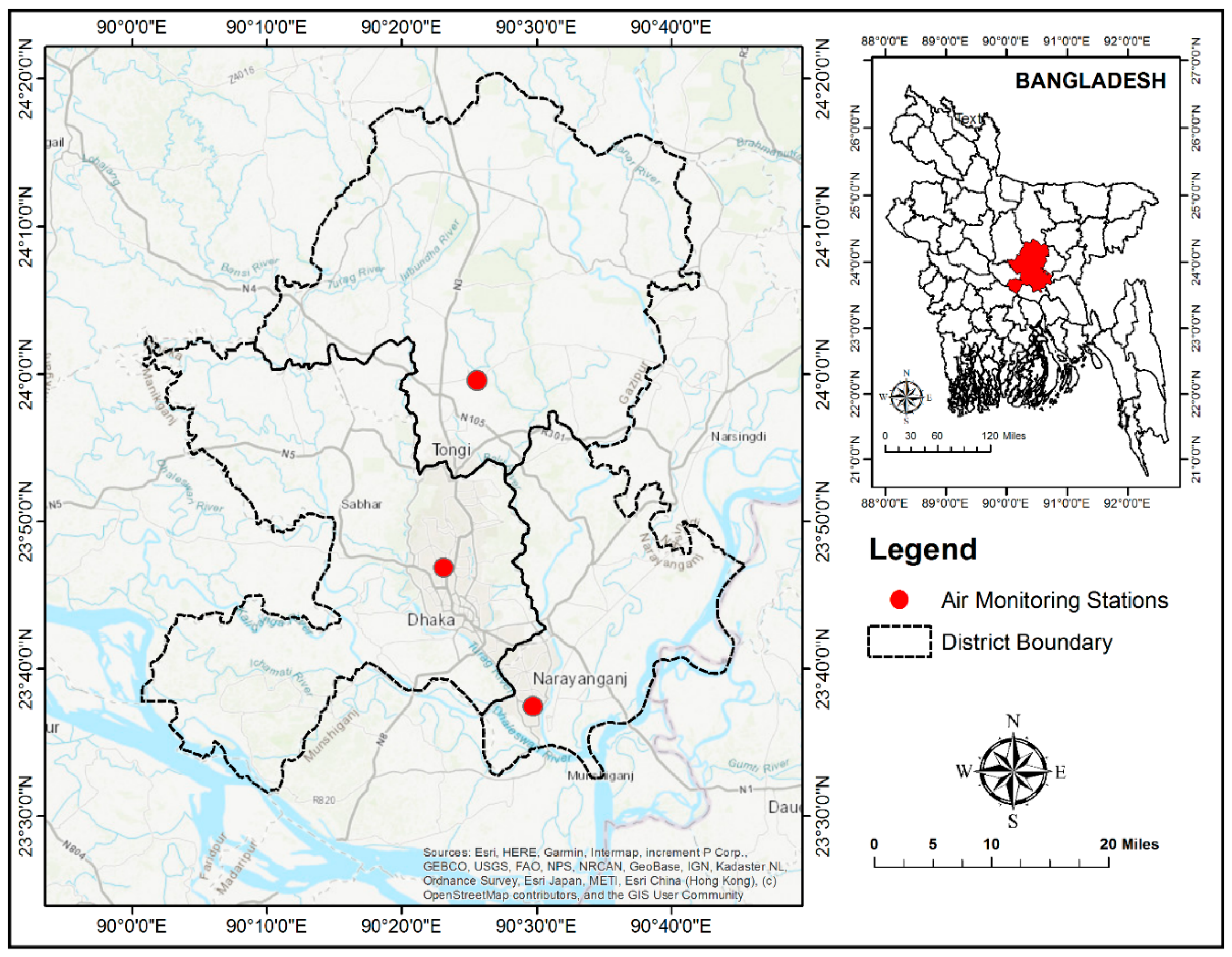
2. Air Monitoring Stations
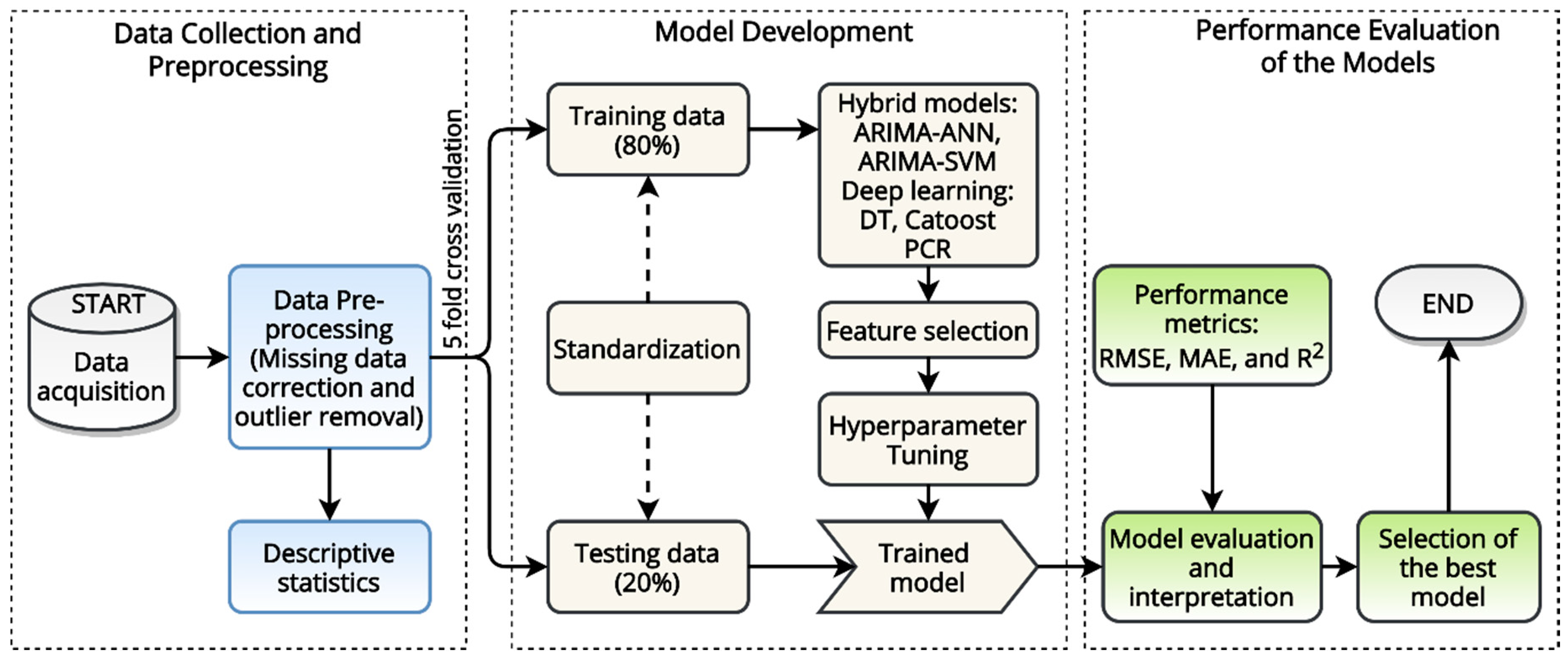
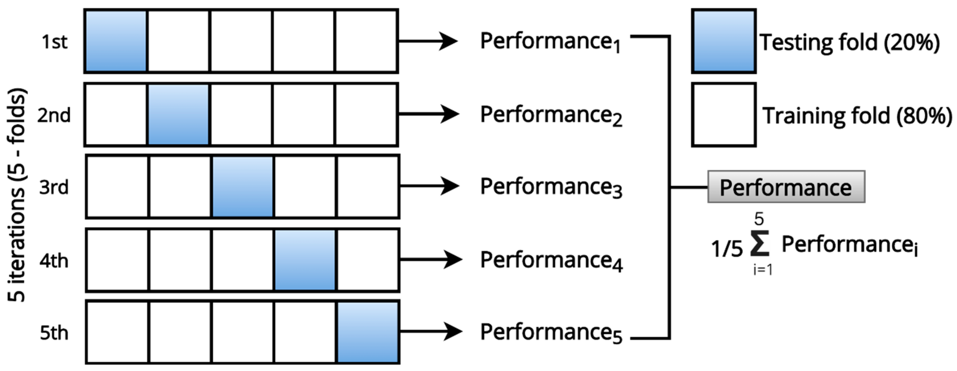
3. Methodology
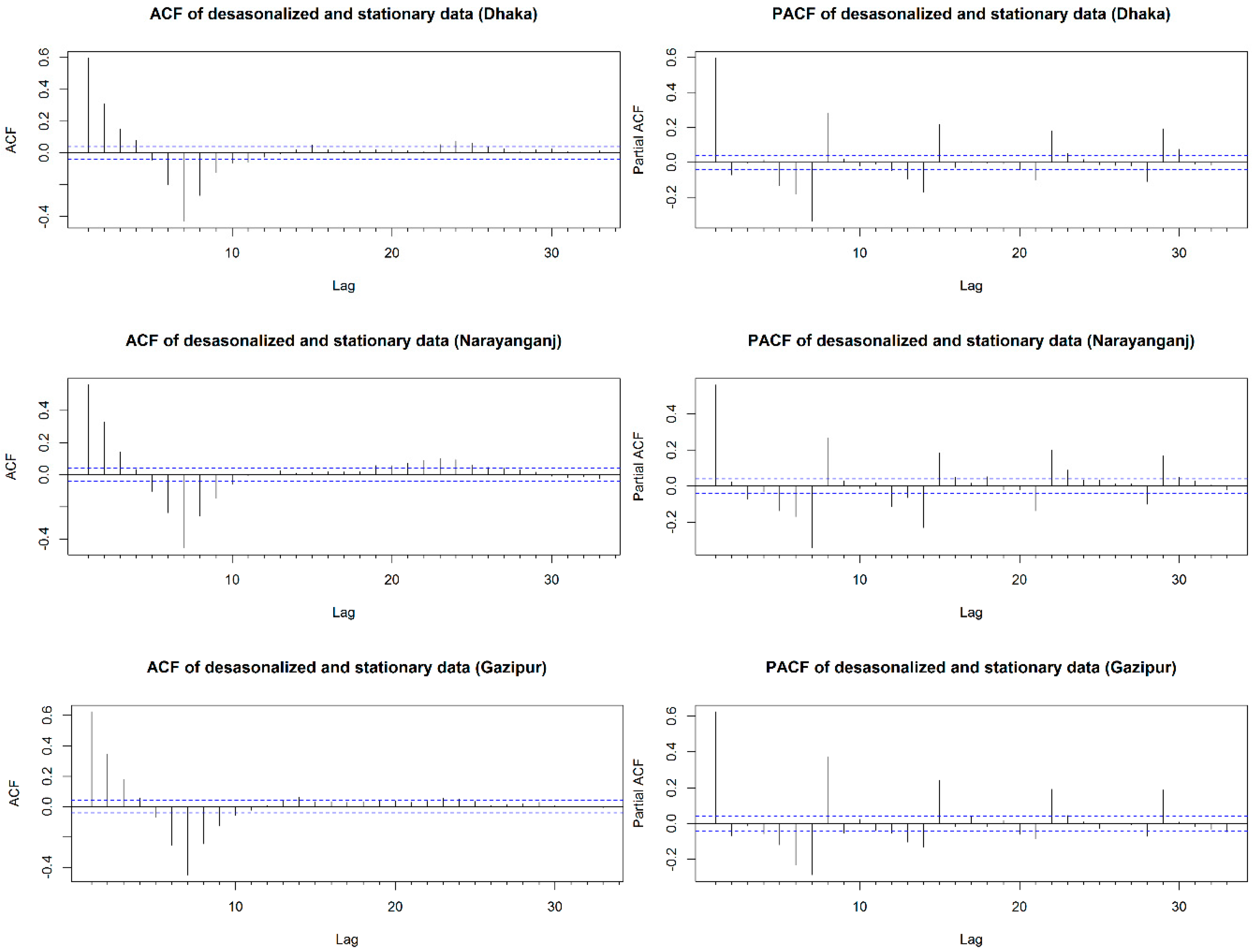
3.1. Pre-Processing
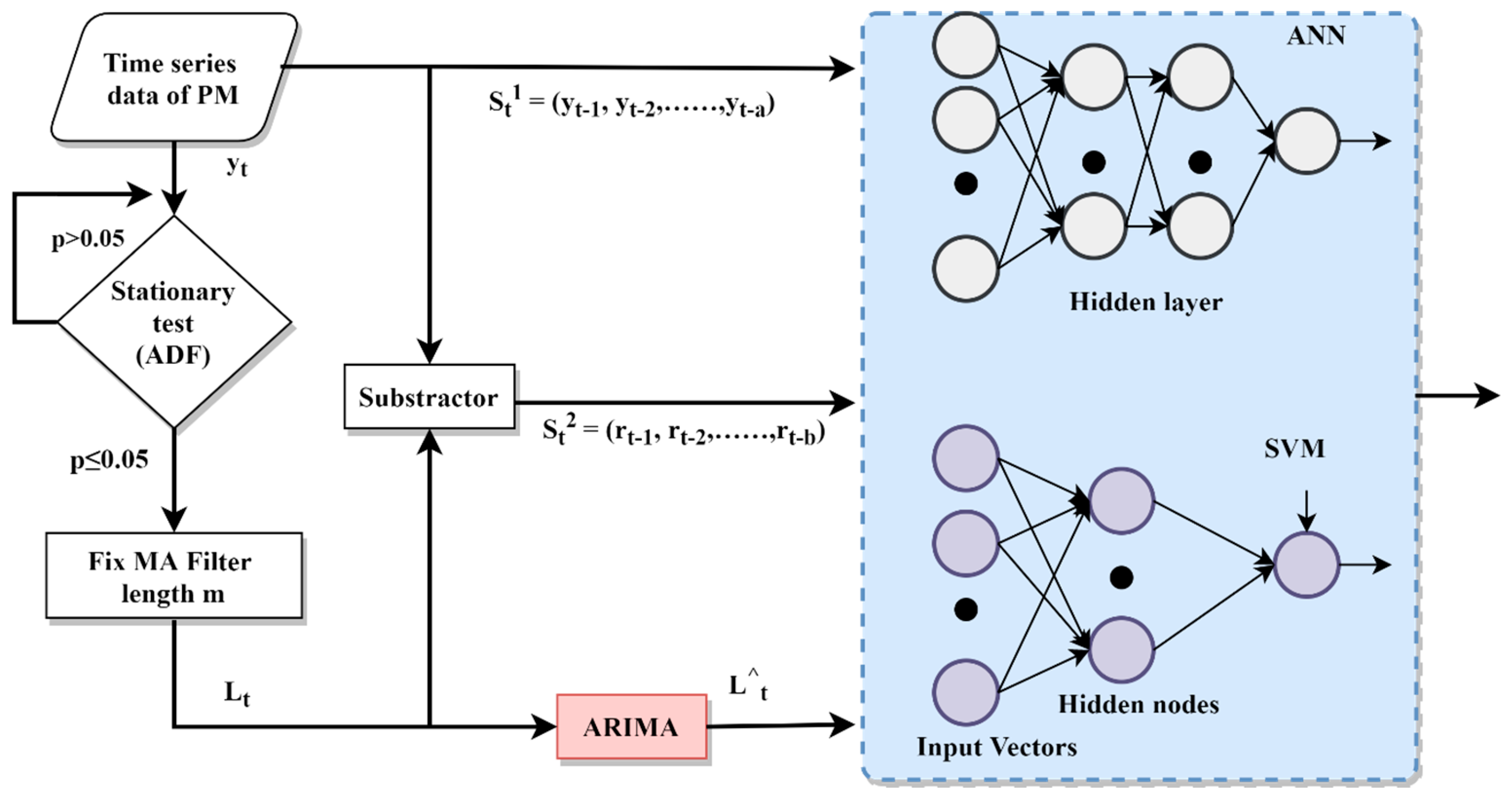
3.2. ARIMA
3.3. Artificial Neural Network (ANN)
3.4. Support Vector Machine (SVM)
3.5. Hybrid Model
3.6. Decision Trees
3.7. CatBoost
3.8. Principle Component Regression
3.9. Empirical Results
4. Results and Discussion
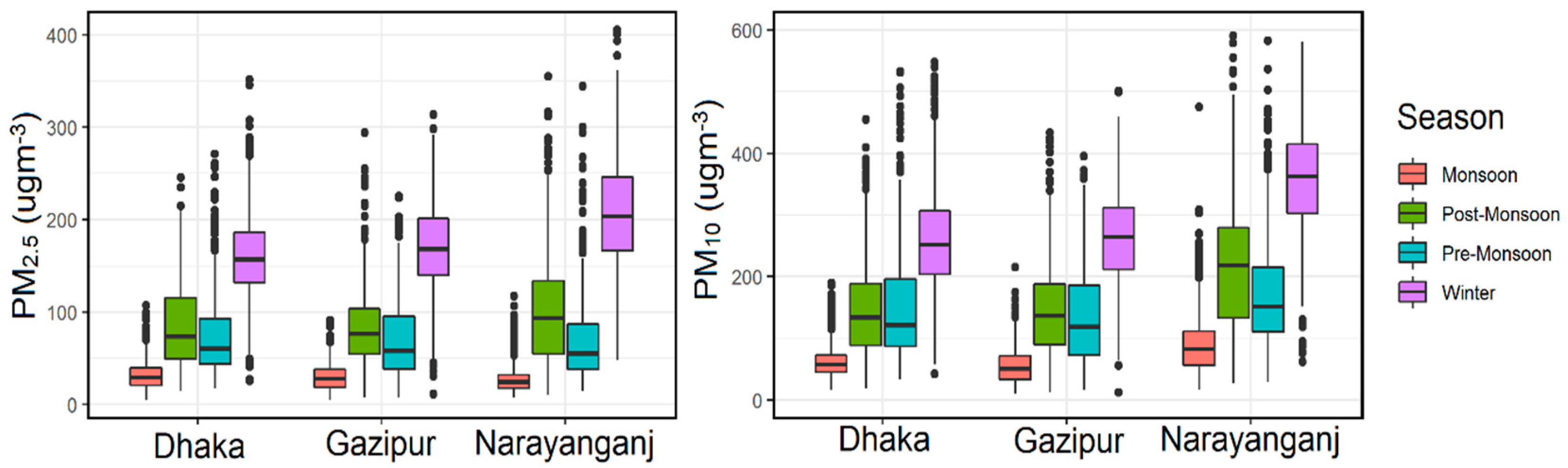
4.1. Descriptive Statistics
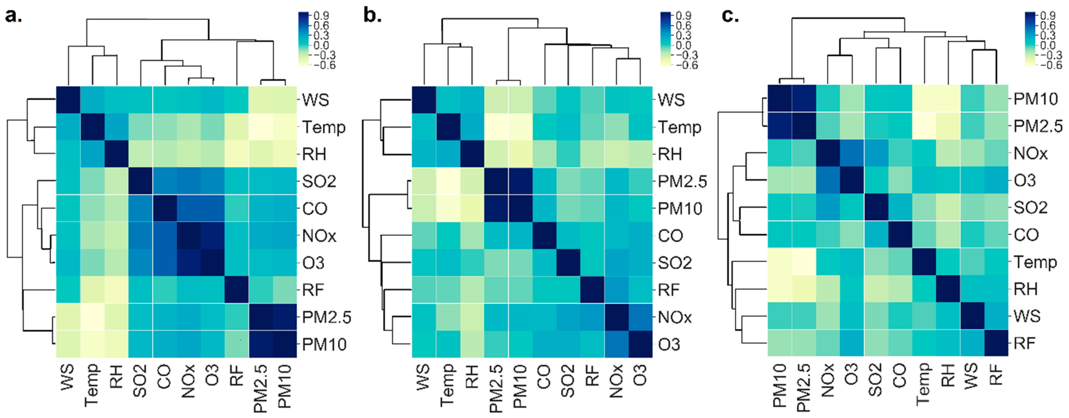
4.2. Local Meteorology and Their Relation to Pollutants
4.3. Results of ARIMA-ANN and ARIMA-SVM
4.4. Result of Decision Tree (DT) and CatBoost
4.5. Results of PCR
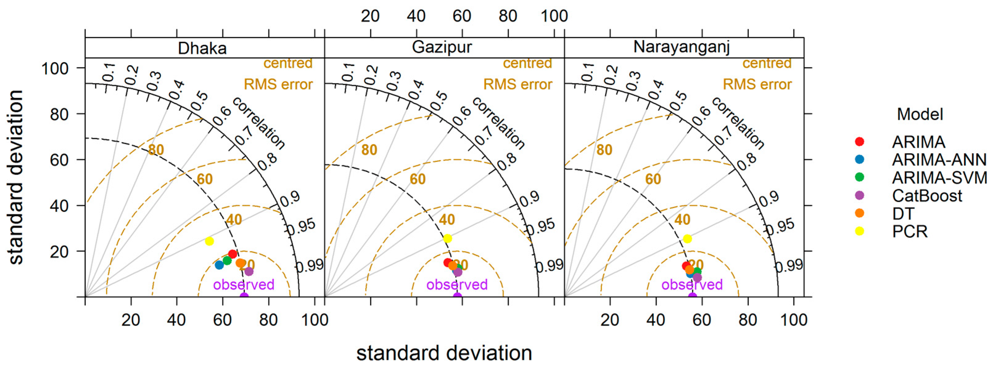
4.6. Comparison of Model Performance
5. Conclusions
Supplementary Materials
Author Contributions
Funding
Acknowledgments
Conflicts of Interest
References
- Manisalidis, I.; Stavropoulou, E.; Stavropoulos, A.; Bezirtzoglou, E. Environmental and Health Impacts of Air Pollution: A Review. Front. Public Health 2020, 8, 14. [Google Scholar] [CrossRef] [Green Version]
- Lv, D.; Chen, Y.; Zhu, T.; Li, T.; Shen, F.; Li, X.; Mehmood, T.; Ying, C. The pollution characteristics of PM10 and PM2.5 during summer and winter in Beijing, Suning and Islamabad. Atmos. Pollut. Res. 2019, 10, 1159–1164. [Google Scholar] [CrossRef]
- Bo, M.; Salizzoni, P.; Clerico, M.; Buccolieri, R. Assessment of Indoor-Outdoor Particulate Matter Air Pollution: A Review. Atmosphere 2017, 8, 136. [Google Scholar] [CrossRef] [Green Version]
- Fuzzi, S.; Baltensperger, U.; Carslaw, K.S.; Decesari, S.; Van Der Gon, H.D.; Facchini, M.C.; Fowler, D.; Koren, I.; Langford, B.; Lohmann, U.; et al. Particulate matter, air quality and climate: Lessons learned and future needs. Atmos. Chem. Phys. Discuss. 2015, 15, 8217–8299. [Google Scholar] [CrossRef] [Green Version]
- Cesari, D.; De Benedetto, G.; Bonasoni, P.; Busetto, M.; Dinoi, A.; Merico, E.; Chirizzi, D.; Cristofanelli, P.; Donateo, A.; Grasso, F.; et al. Seasonal variability of PM2.5 and PM10 composition and sources in an urban background site in Southern Italy. Sci. Total Environ. 2018, 612, 202–213. [Google Scholar] [CrossRef] [PubMed]
- Liu, H.-Y.; Dunea, D.; Iordache, S.; Pohoata, A. A Review of Airborne Particulate Matter Effects on Young Children’s Respiratory Symptoms and Diseases. Atmosphere 2018, 9, 150. [Google Scholar] [CrossRef] [Green Version]
- Choi, S.; Kim, K.H.; Kim, K.; Chang, J.; Kim, S.M.; Kim, S.R.; Cho, Y.; Lee, G.; Son, J.S.; Park, S.M. Association between Post-Diagnosis Particulate Matter Exposure among 5-Year Cancer Survivors and Cardiovascular Disease Risk in Three Metropolitan Areas from South Korea. Int. J. Environ. Res. Public Health 2020, 17, 2841. [Google Scholar] [CrossRef]
- Jaganathan, S.; Jaacks, L.M.; Magsumbol, M.; Walia, G.K.; Sieber, N.L.; Shivashankar, R.; Dhillon, P.K.; Shahulhameed, S.; Schwartz, J.D.; Prabhakaran, D. Association of Long-Term Exposure to Fine Particulate Matter and Cardio-Metabolic Diseases in Low- and Middle-Income Countries: A Systematic Review. Int. J. Environ. Res. Public Health 2019, 16, 2541. [Google Scholar] [CrossRef] [Green Version]
- Yin, P.; Guo, J.; Wang, L.; Fan, W.; Lu, F.; Guo, M.; Moreno, S.B.R.; Wang, Y.; Wang, H.; Zhou, M.; et al. Higher Risk of Cardiovascular Disease Associated with Smaller Size-Fractioned Particulate Matter. Environ. Sci. Technol. Lett. 2020, 7, 95–101. [Google Scholar] [CrossRef]
- Bae, J.-E.; Choi, H.; Shin, D.W.; Na, H.-W.; Park, N.Y.; Kim, J.B.; Jo, D.S.; Cho, M.J.; Lyu, J.H.; Chang, J.H.; et al. Fine particulate matter (PM2.5) inhibits ciliogenesis by increasing SPRR3 expression via c-Jun activation in RPE cells and skin keratinocytes. Sci. Rep. 2019, 9, 3994. [Google Scholar] [CrossRef]
- Bowe, B.; Xie, Y.; Li, T.; Yan, Y.; Xian, H.; Al Aly, Z. Estimates of the 2016 global burden of kidney disease attributable to ambient fine particulate matter air pollution. BMJ Open 2019, 9, e022450. [Google Scholar] [CrossRef] [PubMed]
- Atkinson, R.; Kang, S.; Anderson, R.; Mills, I.; Walton, H. Epidemiological time series studies of PM2.5 and daily mortality and hospital admissions: A systematic review and meta-analysis. Thorax 2014, 69, 660–665. [Google Scholar] [CrossRef] [PubMed] [Green Version]
- Kim, K.-H.; Kabir, E.; Kabir, S. A review on the human health impact of airborne particulate matter. Environ. Int. 2015, 74, 136–143. [Google Scholar] [CrossRef] [PubMed]
- Wu, X.; Nethery, R.C.; Sabath, B.M.; Braun, D.; Dominici, F. Exposure to air pollution and COVID-19 mortality in the United States. medRxiv 2020. [Google Scholar] [CrossRef] [Green Version]
- Lelieveld, J.; Evans, J.S.; Fnais, M.; Giannadaki, D.; Pozzer, A. The contribution of outdoor air pollution sources to premature mortality on a global scale. Nat. Cell Biol. 2015, 525, 367–371. [Google Scholar] [CrossRef]
- Begum, B.A.; Hopke, P.K. Ambient Air Quality in Dhaka Bangladesh over Two Decades: Impacts of Policy on Air Quality. Aerosol Air Qual. Res. 2018, 18, 1910–1920. [Google Scholar] [CrossRef] [Green Version]
- Mahmood, A.; Hu, Y.; Nasreen, S.; Hopke, P.K. Airborne Particulate Pollution Measured in Bangladesh from 2014 to 2017. Aerosol Air Qual. Res. 2019, 19, 272–281. [Google Scholar] [CrossRef]
- Begum, B.A.; Biswas, S.K.; Hopke, P.K. Assessment of trends and present ambient concentrations of PM2.2 and PM10 in Dhaka, Bangladesh. Air Qual. Atmos. Health 2008, 1, 125–133. [Google Scholar] [CrossRef] [Green Version]
- Mitra, N.; Shahriar, S.A.; Lovely, N.; Khan, S.; Rak, A.; Kar, S.; Khaleque, A.; Amin, M.F.M.; Kayes, I.; Salam, M.A. Assessing Energy-Based CO2 Emission and Workers’ Health Risks at the Shipbreaking Industries in Bangladesh. Environment 2020, 7, 35. [Google Scholar] [CrossRef]
- Ibn Azkar, M.A.M.B.; Chatani, S.; Sudo, K. Simulation of urban and regional air pollution in Bangladesh. J. Geophys. Res. Space Phys. 2012, 117, 1–23. [Google Scholar] [CrossRef] [Green Version]
- Salam, M.A.; Shirasuna, Y.; Hirano, K.; Masunaga, S. Particle associated polycyclic aromatic hydrocarbons in the atmospheric environment of urban and suburban residential area. Int. J. Environ. Sci. Technol. 2011, 8, 255–266. [Google Scholar] [CrossRef] [Green Version]
- Ab Kadir, Z.; Yusoff, M.; Awang, N.R.; Jani, M.; Arieff, M.; Selvam, B.; Sulaiman, M.A.; Salam, M.A. Identification of Cation Elements in PM10 Concentration in Industrial Area of Penang. J. Trop. Resour. Sustain. Sci. 2017, 5, 46–50. [Google Scholar]
- Kayes, I.; Shahriar, S.A.; Hasan, K.; Akhter, M.; Kabir, M.M.; Salam, M.A. The relationships between meteorological parameters and air pollutants in an urban environment. Glob. J. Environ. Sci. Manag. 2019, 5, 265–278. [Google Scholar] [CrossRef]
- Rybarczyk, Y.; Zalakeviciute, R. Machine Learning Approaches for Outdoor Air Quality Modelling: A Systematic Review. Appl. Sci. 2018, 8, 2570. [Google Scholar] [CrossRef] [Green Version]
- Jiménez, P.A.; Dudhia, J. On the Ability of the WRF Model to Reproduce the Surface Wind Direction over Complex Terrain. J. Appl. Meteorol. Clim. 2013, 52, 1610–1617. [Google Scholar] [CrossRef]
- Chen, Q.; Taylor, D. Transboundary atmospheric pollution in Southeast Asia: Current methods, limitations and future developments. Crit. Rev. Environ. Sci. Technol. 2018, 48, 997–1029. [Google Scholar] [CrossRef]
- Shimadera, H.; Kojima, T.; Kondo, A. Evaluation of Air Quality Model Performance for Simulating Long-Range Transport and Local Pollution of PM2.5 in Japan. Adv. Meteorol. 2016, 2016, 1–13. [Google Scholar] [CrossRef] [Green Version]
- Chen, J.; Chen, J.Y.; Wu, Z.; Hu, D.; Pan, J.Z. Forecasting smog-related health hazard based on social media and physical sensor. Inf. Syst. 2017, 64, 281–291. [Google Scholar] [CrossRef]
- Yang, G.; Lee, H.; Lee, G. A Hybrid Deep Learning Model to Forecast Particulate Matter Concentration Levels in Seoul, South Korea. Atmosphere 2020, 11, 348. [Google Scholar] [CrossRef] [Green Version]
- Suleiman, A.; Tight, M.; Quinn, A. Applying machine learning methods in managing urban concentrations of traffic-related particulate matter (PM10 and PM2.5). Atmos. Pollut. Res. 2019, 10, 134–144. [Google Scholar] [CrossRef]
- Pakrooh, P.; Pishbahar, E. Forecasting Air Pollution Concentrations in Iran, Using a Hybrid. Model. Pollut. 2019, 5, 739–747. [Google Scholar] [CrossRef]
- Kang, G.K.; Gao, J.; Chiao, S.; Lu, S.; Xie, G. Air Quality Prediction: Big Data and Machine Learning Approaches. Int. J. Environ. Sci. Dev. 2018, 9, 8–16. [Google Scholar] [CrossRef] [Green Version]
- Rana, M.; Sulaiman, N.; Sivertsen, B.; Khan, F.; Nasreen, S. Trends in atmospheric particulate matter in Dhaka, Bangladesh, and the vicinity. Environ. Sci. Pollut. Res. 2016, 23, 17393–17403. [Google Scholar] [CrossRef] [PubMed]
- Islam, M.; Sharmin, M.; Ahmed, F. Predicting air quality of Dhaka and Sylhet divisions in Bangladesh: A time series modeling approach. Air Qual. Atmos. Health 2020, 13, 607–615. [Google Scholar] [CrossRef]
- Shahriar, S.A.; Kayes, I.; Hasan, K.; Salam, M.A.; Chowdhury, S. Applicability of machine learning in modeling of atmospheric particle pollution in Bangladesh. Air Qual. Atmos. Health 2020, 13, 1247–1256. [Google Scholar] [CrossRef] [PubMed]
- Krzyzanowski, M.; Apte, J.S.; Bonjour, S.P.; Brauer, M.; Cohen, A.J.; Prüss-Ustun, A.M. Air Pollution in the Mega-cities. Curr. Environ. Health Rep. 2014, 1, 185–191. [Google Scholar] [CrossRef]
- Barzeghar, V.; Sarbakhsh, P.; Hassanvand, M.S.; Faridi, S.; Gholampour, A. Long-term trend of ambient air PM10, PM2.5, and O3 and their health effects in Tabriz city, Iran, during 2006–2017. Sustain. Cities Soc. 2020, 54, 101988. [Google Scholar] [CrossRef]
- Tang, R.; Zeng, F.; Chen, Z.; Jing-Song, W.; Huang, C.M.; Wu, Z. The Comparison of Predicting Storm-Time Ionospheric TEC by Three Methods: ARIMA, LSTM, and Seq2Seq. Atmosphere 2020, 11, 316. [Google Scholar] [CrossRef] [Green Version]
- Mossad, A.; Alazba, A. Drought Forecasting Using Stochastic Models in a Hyper-Arid Climate. Atmosphere 2015, 6, 410–430. [Google Scholar] [CrossRef] [Green Version]
- Kamiński, B.; Jakubczyk, M.; Szufel, P. A framework for sensitivity analysis of decision trees. Cent. Eur. J. Oper. Res. 2018, 26, 135–159. [Google Scholar] [CrossRef]
- Moret, B.M.E. Decision Trees and Diagrams. Acm Comput. Surv. 1982, 14, 593–623. [Google Scholar] [CrossRef]
- Zhang, Y.; Zhao, Z.; Zheng, J. CatBoost: A new approach for estimating daily reference crop evapotranspiration in arid and semi-arid regions of Northern China. J. Hydrol. 2020, 588, 125087. [Google Scholar] [CrossRef]
- Mat Shukri, M.A.; Yusoff, M.; Awang, N.R.; Jani, M.; Ab Kadir, Z.; Selvam, B.; Sulaiman, M.A.; Salam, M.A. Investigation of relationship between particulate matter (PM2.5 and PM10) and meteorological parameters at Roadside Area of First Penang Bridge. J. Trop. Resour. Sustain. Sci. 2017, 5, 33–39. [Google Scholar]
- Zhang, H.; Wang, Y.; Hu, J.; Ying, Q.; Hu, X.-M. Relationships between meteorological parameters and criteria air pollutants in three megacities in China. Environ. Res. 2015, 140, 242–254. [Google Scholar] [CrossRef] [PubMed]
- Manju, A.; Kalaiselvi, K.; Dhananjayan, V.; Palanivel, M.; Banupriya, G.S.; Vidhya, M.H.; Panjakumar, K.; Ravichandran, B. Spatio-seasonal variation in ambient air pollutants and influence of meteorological factors in Coimbatore, Southern India. Air Qual. Atmos. Health 2018, 11, 1179–1189. [Google Scholar] [CrossRef]
- Haddad, K.; Vizakos, N. Air quality pollutants and their relationship with meteorological variables in four suburbs of Greater Sydney, Australia. Air Qual. Atmos. Health 2020, 1–13. [Google Scholar] [CrossRef]
- Díaz-Robles, L.A.; Ortega, J.C.; Fu, J.S.; Reed, G.D.; Chow, J.C.; Watson, J.G.; Moncada-Herrera, J.A. A hybrid ARIMA and artificial neural networks model to forecast particulate matter in urban areas: The case of Temuco, Chile. Atmos. Environ. 2008, 42, 8331–8340. [Google Scholar] [CrossRef] [Green Version]
- Mehdipour, V.; Stevenson, D.S.; Memarianfard, M.; Sihag, P. Comparing different methods for statistical modeling of particulate matter in Tehran, Iran. Air Qual. Atmos. Health 2018, 11, 1155–1165. [Google Scholar] [CrossRef]
- Fan, J.; Wang, X.; Zhang, F.; Ma, X.; Wu, L. Predicting daily diffuse horizontal solar radiation in various climatic regions of China using support vector machine and tree-based soft computing models with local and extrinsic climatic data. J. Clean. Prod. 2020, 248, 119264. [Google Scholar] [CrossRef]
- Kumar, A.; Goyal, P. Forecasting of air quality in Delhi using principal component regression technique. Atmos. Pollut. Res. 2011, 2, 436–444. [Google Scholar] [CrossRef] [Green Version]
- Zhang, G.P. Time series forecasting using a hybrid ARIMA and neural network model. Neurocomputing 2003, 50, 159–175. [Google Scholar] [CrossRef]
- Babu, C.N.; Reddy, B.E. A moving-average filter based hybrid ARIMA–ANN model for forecasting time series data. Appl. Soft Comput. 2014, 23, 27–38. [Google Scholar] [CrossRef]
- Khashei, M.; Bijari, M. A novel hybridization of artificial neural networks and ARIMA models for time series forecasting. Appl. Soft Comput. 2011, 11, 2664–2675. [Google Scholar] [CrossRef]


| Variables | Unit | Dhaka | Narayanganj | Gazipur | |||
|---|---|---|---|---|---|---|---|
| Mean ± SE | SD | Mean ± SE | SD | Mean ± SE | SD | ||
| PM2.5 | µg m−3 | 90.5 ± 0.05 | 69.1 | 96.3 ± 0.05 | 83.4 | 85.8 ± 0.05 | 67.4 |
| PM10 | µg m−3 | 160.4 ± 0.05 | 110.8 | 202.4 ± 0.05 | 134.4 | 143.8 ± 0.05 | 104.5 |
| SO2 | Ppb | 5.9 ± 0.05 | 5.3 | 7.2 ± 0.05 | 7.9 | 8.9 ± 0.05 | 10.3 |
| CO | Ppm | 1.2 ± 0.05 | 0.6 | 1.6 ± 0.05 | 2.7 | 1.3 ± 0.05 | 0.7 |
| NOx | Ppb | 45.5 ± 0.05 | 36.8 | 21.6 ± 0.05 | 28.8 | 25.1 ± 0.05 | 29.6 |
| O3 | Ppb | 14.04 ± 0.05 | 12.5 | 9.7 ± 0.05 | 10.2 | 10.7 ± 0.05 | 9.9 |
| WS | ms−1 | 2.09 ± 0.05 | 1.1 | 3.5 ± 0.05 | 4.2 | 1.8 ± 0.05 | 1.4 |
| Temp | °C | 26.08 ± 0.05 | 4.5 | 26.7 ± 0.05 | 4.6 | 25.9 ± 0.05 | 4.6 |
| RH | % | 68.6 ± 0.05 | 10.8 | 70.3 ± 0.05 | 9.6 | 73.08 ± 0.05 | 12.5 |
| RF | Mm | 0.7 ± 0.05 | 2.1 | 0.2 ± 0.05 | 0.4 | 0.6 ± 0.05 | 1.06 |
| Test Component | Dhaka | Narayanganj | Gazipur |
|---|---|---|---|
| Test Statistic value | −3.9905 | −3.9428 | −3.7972 |
| p-value | 0.01 | 0.01 | 0.02 |
| Monitoring Station | Model | Coefficient | Estimate | SE |
|---|---|---|---|---|
| Dhaka | (3,0,2) (2,0,2) [10] | AR1 | 0.4530 | 0.0511 |
| AIC = 14,329.3 | AR2 | 0.8592 | 0.0408 | |
| BIC = 14,392.5 | AR3 | 1.0126 | 0.0503 | |
| RMSE = 19.30 | MA1 | 1.1239 | 0.0749 | |
| MAE = 11.37 | MA2 | 0.3707 | 0.0478 | |
| SAR1 | 0.3892 | 0.1472 | ||
| SAR2 | −0.7386 | 0.1053 | ||
| SMA1 | −0.3827 | 0.1378 | ||
| SMA2 | 0.7786 | 0.0951 | ||
| Narayanganj | (3,0,2) (2,0,1) [10] | AR1 | 0.3013 | 0.0254 |
| AIC = 15,371.32 | AR2 | 0.0725 | 0.0199 | |
| BIC = 15,423.12 | AR3 | 0.4892 | 0.0494 | |
| RMSE = 17.52 | MA1 | 0.3933 | 0.0249 | |
| MAE = 10.01 | MA2 | 0.4063 | 0.0425 | |
| SAR1 | 0.5244 | 0.0503 | ||
| SAR2 | −0.0035 | 0.0249 | ||
| SMA1 | 0.0632 | 0.0349 | ||
| Gazipur | (3,0,2) (1,0,1) [10] | AR1 | 0.5521 | 0.0344 |
| AIC = 13,842.38 | AR2 | 0.8844 | 0.0341 | |
| BIC = 13,882.67 | AR3 | −0.4515 | 0.0353 | |
| RMSE = 19.95 | MA1 | 1.1426 | 0.0550 | |
| MAE = 11.07 | MA2 | 0.2478 | 0.0539 | |
| SAR1 | −0.8465 | 0.0940 | ||
| SMA1 | 0.8201 | 0.1005 |
| Station | Performance Indicator | Models | ||||
|---|---|---|---|---|---|---|
| ARIMA-ANN | ARIMA-SVM | DT | CatBoost | PCR | ||
| Dhaka | RMSE | 11.96 | 14.03 | 12.27 | 11.41 | 25.37 |
| MAE | 6.78 | 8.51 | 6.74 | 5.82 | 14.23 | |
| R2 | 0.93 | 0.91 | 0.88 | 0.95 | 0.81 | |
| Narayanganj | RMSE | 12.86 | 13.97 | 13.07 | 12.56 | 26.87 |
| MAE | 7.64 | 8.31 | 7.95 | 6.97 | 18.73 | |
| R2 | 0.90 | 0.89 | 0.89 | 0.92 | 0.78 | |
| Gazipur | RMSE | 12.34 | 12.68 | 14.21 | 12.07 | 25.49 |
| MAE | 7.69 | 7.23 | 7.97 | 5.72 | 17.58 | |
| R2 | 0.91 | 0.89 | 0.87 | 0.94 | 0.79 | |
Publisher’s Note: MDPI stays neutral with regard to jurisdictional claims in published maps and institutional affiliations. |
© 2021 by the authors. Licensee MDPI, Basel, Switzerland. This article is an open access article distributed under the terms and conditions of the Creative Commons Attribution (CC BY) license (http://creativecommons.org/licenses/by/4.0/).
Share and Cite
Shahriar, S.A.; Kayes, I.; Hasan, K.; Hasan, M.; Islam, R.; Awang, N.R.; Hamzah, Z.; Rak, A.E.; Salam, M.A. Potential of ARIMA-ANN, ARIMA-SVM, DT and CatBoost for Atmospheric PM2.5 Forecasting in Bangladesh. Atmosphere 2021, 12, 100. https://0-doi-org.brum.beds.ac.uk/10.3390/atmos12010100
Shahriar SA, Kayes I, Hasan K, Hasan M, Islam R, Awang NR, Hamzah Z, Rak AE, Salam MA. Potential of ARIMA-ANN, ARIMA-SVM, DT and CatBoost for Atmospheric PM2.5 Forecasting in Bangladesh. Atmosphere. 2021; 12(1):100. https://0-doi-org.brum.beds.ac.uk/10.3390/atmos12010100
Chicago/Turabian StyleShahriar, Shihab Ahmad, Imrul Kayes, Kamrul Hasan, Mahadi Hasan, Rashik Islam, Norrimi Rosaida Awang, Zulhazman Hamzah, Aweng Eh Rak, and Mohammed Abdus Salam. 2021. "Potential of ARIMA-ANN, ARIMA-SVM, DT and CatBoost for Atmospheric PM2.5 Forecasting in Bangladesh" Atmosphere 12, no. 1: 100. https://0-doi-org.brum.beds.ac.uk/10.3390/atmos12010100