Article

A Computational Methodology for the Calibration of Tephra Transport Nowcasting at Sakurajima Volcano, Japan

by
Alexandros P. Poulidis
1,*,
Atsushi Shimizu
2,
Haruhisa Nakamichi
1 and
Masato Iguchi
1
1
Sakurajima Volcano Research Center, Disaster Prevention Research Institute, Kyoto University, Kagoshima 891-1419, Japan
2
Center for Regional Environmental Research, National Institute for Environmental Studies, Tsukuba 305-8506, Japan
*
Author to whom correspondence should be addressed.
Submission received: 9 December 2020 / Revised: 4 January 2021 / Accepted: 8 January 2021 / Published: 12 January 2021

Abstract

:
Ground-based remote sensing equipment have the potential to be used for the nowcasting of the tephra hazard from volcanic eruptions. To do so raw data from the equipment first need to be accurately transformed to tephra-related physical quantities. In order to establish these relations for Sakurajima volcano, Japan, we propose a methodology based on high-resolution simulations. An eruption that occurred at Sakurajima on 16 July 2018 is used as the basis of a pilot study. The westwards dispersal of the tephra cloud was ideal for the observation network that has been installed near the volcano. In total, the plume and subsequent tephra cloud were recorded by 2 XMP radars, 1 lidar and 3 optical disdrometers, providing insight on all phases of the eruption, from plume generation to tephra transport away from the volcano. The Weather Research and Forecasting (WRF) and FALL3D models were used to reconstruct the transport and deposition patterns. Simulated airborne tephra concentration and accumulated load were linked, respectively, to lidar backscatter intensity and radar reflectivity. Overall, results highlight the possibility of using such a high-resolution modelling-based methodology as a reliable complementary strategy to common approaches for retrieving tephra-related quantities from remote sensing data.

1. Introduction

Tephra released after volcanic eruptions constitutes a persistent hazard for communities around them [1,2,3,4]. This has been the case for Sakurajima volcano in Japan [5]. Located on the island of Kyushu in southern Japan (31.58° N, 130.65° E, peak height 1117 m; Figure 1a), the volcano has been active since 1955, with a major impact on agriculture of ∼236 billion yen between 1978 and 2017 [5]. Due to its frequent activity [6,7] and to the potential impact on human settlements and activities from large eruptions [8], Sakurajima is one of Japan’s most closely monitored volcanoes [5,9].
In order to monitor tephra dispersal, the Sakurajima Volcanological Observatory (SVO), part of the Disaster Prevention Research Institute of Kyoto University, has installed a network of XMP radars, lidars and optical disdrometers to monitor plumes, tephra transport and sedimentation [5], whose positioning is shown in Figure 1b. XMP radars provide a way of monitoring the transport of tephra over large areas, with the drawback of neglecting fine particles due to the wavelengths employed [10,11,12,13,14,15,16]. On the other hand, lidars can be used to monitor the presence of fine particles [17,18,19], but the sampled area is limited to a line (at Sakurajima pointing from the SVO towards the crater). Finally, disdrometers have been shown to be valuable in the monitoring of tephra sedimentation [20,21], but carry similar limitations to the radars, that is, the wavelength employed limits observations of particles with diameters below ∼0.2 mm [21,22,23]. Despite the limitations of individual equipment, this observational network, coupled with numerical modelling of tephra dispersal [20,21,24], allows for reliable and detailed monitoring of tephra transport from Sakurajima.
To establish a real-time nowcasting system, a crucial component is the transformation of raw data output to meaningful parameters for hazard monitoring, such as tephra concentration and sedimentation estimates. Default estimates based on hydrometeors are inapplicable in the case of tephra, which is solid and features complex morphology [25]. The Volcanic Ash Radar Retrieval (VARR) model was created to link radar output data (specifically radar reflectivity; Z H H ) to deposit load, which is especially useful when dealing with eruptions with a lack of in-situ data for validation [10]. The algorithm represents a significant milestone in radar observations of tephra and has been successfully applied for tephra-fall observations [26] and expanded, for example via the inclusion of other radar parameters, such as the specific phase shift ( K D P ) [16]. Still, the VARR algorithm is based on assumptions regarding the particle distribution and the microphysical model employed which, although easy to amend with the accumulation of new data, can still be difficult to validate [10].
Numerical tephra transport and deposition (TTD) models are another commonly used tool when it comes to tephra monitoring [27]. Based on certain initial parameters for each eruption (commonly referred to as Eruptive Source Parameters; ESPs), TTD models allow us to gain insight on the dispersal of tephra with spatial and temporal detail that is impossible to achieve with remote sensing and sample collecting alone. In recent years the refinement of numerical models [27,28,29] and an increased capability to constrain ESPs [30,31] has led to an improvement in the accuracy of TTD modelling. In the case of Sakurajima volcano, high-resolution tephra transport simulations can be carried out with an error commonly contained within a factor between 2–4 [20,21]. If we assume these errors representative for the whole dispersal area, model results could potentially be used as a link between remote sensing and tephra fallout.
The question of whether such a modelling-based methodology can be used to establish a relation between radar and lidar data and tephra-related quantities is explored here. As a first step, an eruption that occurred at Sakurajima on 16 July 2018 is used as a proof of concept, chosen as the wind profile on the day led to the westwards transport of the tephra cloud, an ideal direction for sampling through the installed equipment (Figure 1b). Initially, observational data (introduced in Section 2) are used to gain insight on the eruption and subsequent tephra dispersal (Section 3) and after that a relation between the model and remote-sensing data is explored in Section 5. A discussion of the results in the context of tephra hazard management is included in Section 6 and the paper concludes with a summary of the main finding (Section 7).

2. Observational Equipment

The study used data from 2 XMP radars (WR2100, Furuno, operating frequency 9.4 GHz or 3.2 cm wavelength; Figure 1b) focused on Sakurajima: 1 scanning horizontally located at Hirakawa city (∼20 km to the southwest; diamond marker in Figure 1b), and 1 radar scanning vertically, located at the SVO (∼6 km to the west of the vent; square marker in Figure 1b). Radar data are captured at a total of 7 elevations (2°, 5°, 10°, 15°, 20°, 25° and 30°) every 1 min in the case of the Hirakawa radar and 11 azimuth angles (95° to 115° at a 2° interval) every ∼72 s for the SVO radar. Noise and ground clutter were removed from the radar data using the assumptions presented in Reference [16], that is, data used were chosen based on radar reflectivity ( Z H H > 0 ), doppler velocity ( V 0 m s−1), differential reflectivity (−3 Z D R 3) and corporal correlation ( ρ 0.6 ).
The lidar used is a polarization dual-wavelength lidar (FIT Leadintex), which radiates linearly polarized light pulses at wavelength of 532 and 1064 nm. Both parallel and perpendicular components of backscatter are detected for the 532 nm wavelength, while only the total backscatter is detected for the 1064 nm wavelength. Note that in this study only data from the first two channels, that is, the 532 nm wavelength were used. The light pulse is radiated 40 times in the first 2 s and after 8 s, 40 pulses are radiated again. The sequence is repeated with a time interval of 10 s. The lidar backscatter intensity was calculated as I 532 = I + I and the depolarisation ratio as D 532 = I / I . The raw data for I were divided by 1010 to produce the arbitrary units shown here.
Particle-Size-Velocity (parsivel) optical disdrometers (OTT Parsivel2) were used to observe tephra sedimentation. Although disdrometers are most commonly used for measuring the size and fall velocity of hydrometeors (e.g., rain [32] and snow [33]), multiple studies have highlighted their usefulness in tephra fallout monitoring [15,22,23]. The OTT Parsivel2 disdrometers work by measuring a voltage change when particles pass through a 54 cm2 detection area composed of a horizontal strip of a laser beam with a wavelength of 650 nm and can observe solid particles with diameters between 0.2–25 mm [22,23] and fall speeds between 0.2–20 m s−1. A sampling rate of 1 min was used in the study.

3. The 16 July 2018 Eruption

3.1. Observed Characteristics

The vulcanian eruption from Minamidake crater under study occurred during the evening of 16 July 2018: starting at 1538 JST (Japan Standard Time; JST = UTC + 9) it lasted for approximately 5 min, leading to an estimated release of 107 kg of tephra, based on geophysical monitoring of the volcano [7,9] (Figure 2a). The reported plume height ( H P ) by the Japan Meteorological Agency (JMA) was 4.6 km above the vent and easterly winds led to westwards dispersal of the tephra cloud towards the city of Kagoshima, with tephra sedimentation observed at three disdrometer locations. The radar data from the vertically-scanning radar at the SVO show high values of Z H H up to a maximum height of 4 km agl at the time of the eruption (Figure 2b), slightly below the reported H P . This underestimation of H P was also noted in a previous study on Sakurajima [21]. Weaker emissions continued for an hour after the eruption with a maximum height between 1–1.5 km.
The transport of the tephra cloud was recorded clearly in the lidar data (Figure 2c). Between 1545–1600 JST, lidar backscatter intensity values shifted towards the lidar, with an average horizontal velocity of ∼6 m s−1. Backscatter intensity (I) critically depends on the backscatter coefficient ( β ) and the round trip attenuation by optical depth ( e 2 τ , where τ is the optical depth), with both quantities being proportional to the surface area of the particles. As such, if a dense aerosol layer exists near the lidar, I is strongly decreased as τ increases, meaning that particles near the lidar can occlude the presence of particles behind them.
This can be confirmed via the lidar depolarisation ratio which reveals that a layer of non-spherical particles extends at least 4 km away from the lidar until ∼1640 JST (Figure 2d). Based on Mie scattering theory [34], the depolarization ratio (i.e., perpendicular component in backscatter) should equal zero. However, Mie scattering theory is applicable for a sphere whose refractive indices are homogeneous. If the observed depolarization ratio is non-zero, this assumption is not satisfied. In such case the shape of the particle is considered to be far from a perfect sphere [35], which is true in the case of tephra.
The combination of radar data from the SVO (vertical) and Hirakawa (horizontal) allows for the detailed examination of the plume evolution and the advection of the tephra cloud. The initial phase of the eruption lasted for ∼10 min during which tephra transport was dominated by plume dynamics. Within three minutes from the eruption the main bulk of the thermal was contained between 2–3 km asl (Figure 3a). At this point the plume was rising vertically, leading to similar Z H H patterns at both 10° and 5° elevations from the Hirakawa radar (Figure 3f,k). Within the next 4 min, the plume top has tilted towards a horizontal alignment (Figure 3b). Increased Z H H values are seen as vertically-aligned stripes (e.g., at x = −2 km). In the later phase of the eruption tephra dispersal was dominated by the wind: between 1550–1600 JST, the tephra cloud was advected westwards as the top of the cloud and Z H H values decreased (Figure 3c–e). Wind shear caused by the flow around the volcano skewed the top and bottom parts of the plume, with the 5° elevation Z H H signal (Figure 3f–j) shifted by 1 km to the south and 1 km to the east compared to the 10° signal (Figure 3k–o). By 1600 JST the tephra cloud had decreased below the 10° elevation level (Figure 3j), while low Z H H values persisted mainly 1 km asl (Figure 3e,o).
Tephra sedimentation was observed at three disdrometer stations, mainly between 1550–1630 JST (Figure 2a). The observed distributions of particle size and fall velocity differs significantly depending on the location relative to the vent (Figure 4). Sedimentation over Hikinohira (HIK) occurred in two distinct waves, between 1500–1605 and 1610–1630 JST (Figure 2a). Both sedimentation events involved particles with sizes between 0.3–1.1 mm and velocities between 0.9–2 m s−1—characteristics commonly associated with tephra aggregates [21,36,37]. On the other hand, sedimentation over the Akamizu (AKA) site occurred as one event, between 1500–1615 JST with a single maximum at 1603JST (Figure 2a). The size-velocity distribution indicates the existence of denser aggregates, with an estimated density ( ρ A ) of 1000 kg m−3, along with single particles with ρ A = 2000 kg m−3 (Figure 4). Particle sizes ranged between 0.3–1.1 mm and velocities ranged between 1.1–4.9 m s−1. Finally, at Haruta (HAR) sedimentation occurred late, mainly between 1620–1630 JST (Figure 2a). The observed sizes were between 0.25–0.75 mm and velocities between 0.9–2.9 m s−1 indicate the sedimentation of aggregates with ρ A between 400–1000 kg m−3.

3.2. Interpretation of the Eruption and Tephra Transport Data

The combination of radar, lidar and disdrometer data allows for a detailed interpretation of the different eruption stages. During the initial plume dynamics-dominated phase, the majority of the erupted mass was ejected within 3 min and rose vertically for 2 km as seen in the radar data. The main thermal then started tilting towards the horizontal, following theoretical expectations [15,39]. After the tilt, the upper part of the thermal continued expanding vertically and was associated with a weaker Z H H signal, while the bottom part of the plume formed a finger [15,40] at approximately 2 km west of the vent. Considering the timing and low fall velocities registered during the first sedimentation event over HIK, it can be assumed to have been influenced by this finger deposition. In the later phase wind advection was dominant and lacked the creation of new fingers. The tephra cloud was advected westwards with an average velocity between ∼6–7 m s−1, based on the lidar data as well as the timing of the sedimentation over the AKA disdrometer, located 5 km west of the vent. Advection of the top of the cloud was westwards but changing wind direction with height led to a south-western component as tephra descended closer to the surface.
Sedimentation was markedly different based on the location of the disdrometer sites. Sedimentation along the main advection axis (over AKA) involved single particles and dense aggregates. On the other hand, sedimentation from the plume margins mainly involved low-density aggregates (HIK, HAR). Especially, in the case of HAR, considering the relatively short distance from the vent (∼3 km), the timing (∼40 min after the eruption) and the 6 m s−1 average advection velocity, it can be assumed that tephra registered was affected by surface-level local circulation on the lee (i.e., west) side of the volcano, leading to the lateral spread of tephra from the main advection axis, similarly to what was reported in Reference [21]. Evidence of the tephra cloud lingering on the leeside slopes can also be found in the lidar data, that show low-level backscatter intensity values and depolarisation ratio values above the background level for more than 1 h after the eruption.

4. Computational Methodology

4.1. Model Domains and Physical Parametrisation Schemes

Version 4 for the Weather Research and Forecasting (WRF) model [41] was used to provide the initialisation meteorological data for FALL3D (version 8; [28,29]), a state-of-the-art 3D time-dependent Eulerian tephra transport model. Incorporating the effect of the changing wind in the tephra transport modelling has been shown to increase accuracy in tephra transport modelling [42]. Although FALL3D is an offline model, simulations here were carried out in a quasi-online manner by using a high output rate in WRF [20,21]. For the horizontal resolution used in the meteorological modelling, a 10 min output rate captured most of the resolved variability in the wind field due to the better representation of the topography [43] and allowed for comparison against the radar and lidar data.
The European Centre for Medium-Range Weather Forecasts (ECMWF) reanalysis dataset (ERA5 [44]) was used to initialise high-resolution simulations with a horizontal grid resolution down to 300 m. Output data from WRF are used to initialise the FALL3D simulations. This is a commonly used modelling approach both in an operational [45,46] and a research setting [47,48,49] that has been shown to provide accurate results for eruptions from Sakurajima [20,21].
The simulations were initialized using the ERA5 reanalysis dataset ( Δ x 31 km, 137 vertical levels, hourly output [44]). In total 3 two-way nested domains were used with horizontal grid spacing decreasing from 7.5 km (151 × 151 grid points; Δ t = 30 s), to 1.5 km (301 × 301 grid points; Δ t = 6 s) and finally to 0.3 km (376 × 426 grid points; Δ t = 0.167 s) for the innermost domain (Figure 5a). The Shin-Hong scale-aware Planetary Boundary Layer (PBL) scheme [50] was used to parametrise turbulent motion in the innermost domain as at Δ x = 300 m it falls within the “turbulence gray zone” [51]. Other than the PBL scheme, a full physics-paramterisation set was used: hydrometeor microphysics [52], long- and short-wave radiation [53], a surface layer scheme [54], and a land surface model [55]. NWP simulations were carried out for 18 h, while TTD simulations were carried out for 83 min starting at 1537JST. The same grid spacing is used for the FALL3D simulations. In the vertical, 58 vertical levels were used, with vertical grid spacing at 50 m from the surface up to 1 km asl, increasing to a spacing of 1 km near the top of the domain at 50 hPa (∼21 km).

4.2. Eruption Source Parameters and Plume Insertion

The ESPs, that is, the timing ( T E ) and duration ( D E ) of the eruption, the plume height ( H P ) and/or the mass discharge rate ( M . ) and the total grain-size distribution (TGSD; the size distribution of tephra released from the eruption), are critical for the correct reproduction of the TTD after an eruption. Here, the timing, duration and total mass were constrained using geophysical observations (seismicity and inflation; [9]), introducing 1.7 × 10⁷ kg over 5 min at a constant rate of M . = 5.4 × 10⁴ kg s. For the TGSD an empirical formula based on past eruptions from several volcanoes with well-constrained TGSDs [56] and successfully tested for eruptions from Sakurajima [21] was used to provide an estimate for 8 tephra bins with diameters (d) between 8 and 0.063 mm (grain size Φ = −3–4; d[in mm] = 2Φ). For a magma viscosity ( η ) of 105 Pa s and an H P of 4.6 km, the estimated distribution (Figure 5b) featured a secondary peak at Φ = −1 and the larger amount of fine tephra (∼35%). The Ganser model [57] is used to assign a terminal velocity depending on the size, density, and shape of each class, which is added to the atmospheric vertical velocity to determine the fall velocity of each bin. In order to account for aggregation the approach of Sulpizio et al. [58] was used, converting 20% of tephra from all bins with diameters less than 0.51 mm to a new bin with 0.51 mm diameter and 400 kg m−3 density, based on the disdrometer results (Figure 4).
Due to the transient nature of the eruption under study [59] the vertical profile of tephra in the model represents a challenge, as common 1D models (e.g., the FPLUME model which is integrated in FALL3D [60]) assume a steady-state plume. Here, we used a simple strategy based on the Suzuki plume model [38] and the SVO radar data (Figure 2b and Figure 3a–e). Close to the vent, the radar data showed a bottom-heavy profile for the plume (Figure 5c). This can be expected as radar reflectivity is heavily influenced by large particles and cannot register fine particles [10]. We assume that the underestimation of the plume height in the radar data is tied to this inability to record fine particles. In order to reconstruct the lower part of the plume (with a maximum between 0.5–1.5 km agl) and also account for the reported H P we inserted each individual bin as a different Suzuki-type plume, with plume heights between 4.7 km (fine tephra, Φ = 4) linearly decreasing to 1 km ( Φ = −3). To do this, 1 simulation was carried out for every individual bin and results for the 8 simulations were summed up before the analysis to create a “total” FALL3D simulation. This methodology allowed the inserted plume to reflect the radar observations above the vent (Figure 5c) and provided a good match against the reported H P and the observed transport and sedimentation patterns. However, this approach is only applicable here because plume dynamics and tephra particle microphysics that would rely on the total tephra concentration (such as finger sedimentation [61] or aggregation [62]) were not employed, leaving the results for each bin independent from the others.

5. Simulated Transport and Sedimentation

5.1. Model Results

The simulated tephra transport adheres to the expectations described in Section 3.2 (Figure 6). Advection in the model occurred towards the west with a southwards shift between the top and the bottom of the plume (Figure 6a–c). The top of the plume (mainly composed of fine tephra) was advected away from the volcano by 1623 JST (Figure 6d), while part of the tephra cloud lingered over the leeside of the volcano until the end of the simulation due to low wind values (Figure 6f).
Sedimentation generally followed the advection of the lower part of the plume, with no accumulated tephra load over 8 g m−2 in the northern part of the volcano. This can be expected as the plume profile used in the simulations mainly introduced large tephra towards the bottom part of the plume (see Section 4.2). Overall there was little lateral spread in the sedimentation pattern, with the affected area contained within 4 km in the S-N direction.
The simulated sedimentation was in line with the disdrometer observations. Sedimentation at the HIK disdrometer started approximately 15 min after the eruption, followed by sedimentation over the AKA disdrometer ∼25 min after the eruption, mirroring the order of the observed maxima. Sedimentation over HAR occurred late in the simulation (after 1623 JST, Figure 6d,e) and was associated with the lingering tephra cloud. Overall, the simulated total accumulated load (L) is comparable with observed data for most of the disdrometers, since the ratio between modelled and observed data is 0.8 model to observation ratio at HIK (241 to 289 g m−2), 0.45 at AKA (267 to 589 g m−2) and 0.17 at HAR (6 to 33 g m−2).

5.2. Model and Observation Comparison

In order to explore a relation between the model and radar data we focused on the total accumulated deposition. In the case of modelling this meant the total load at the end of the simulation (Figure 7a), while in the case of the radar data we used the maximum radar reflectivity with respect to time as a proxy of the total sedimentation [21]. In order to integrate results from the two radars using multiple elevations and angles, initially the radar data were converted to point values in 3D space. Based on the point values, the Matlab g r i d d a t a ( ) function was then used to linearly interpolate the data onto the same grid used for the FALL3D simulation to allow for a direct comparison. Finally, the maximum Z H H value with respect to height was calculated to act as a proxy of the maximum sedimentation in the horizontal plane (Figure 7b). A scatter plot of the logarithm of the total accumulated deposition was compared to the derived Z H H maximum, illustrating the possibility of deriving a linear relation (Figure 7c).
In an effort to properly assess the error of the relationship to be derived we followed a bootstrapping data selection approach [63] to separate the data to randomly chosen training and validation datasets. The training dataset (166 points; 70% of the total) was used to form the relation using linear regression, while the validation dataset (70 points; 30% of the total) was used to calculate the error statistics. Using linear regression on the training dataset resulted to the following equation:
l o g 10 ( L ) = Z H H 0.088 0.787 .
Using the validation dataset the Root Mean Square Error (RMSE) was estimated at 0.7 and the Mean Bias Error (MBE) was estimated at 0.03. As the relation is between the logarithm of L, an RMSE of 0.7 amounts to a ∼0.5 order of magnitude error. Note that only data points with Z H H 10 dBz and L 10 0 g m−2 were used in the calculations.
For the lidar observations, model data of tephra concentration were interpolated along the lidar beam coordinates (Figure 8c) and the lidar data were upscaled to the resulting model grid (∼300 m spacing; Figure 8a). Due to the physics of the lidar observations, a direct comparison of the backscatter intensity (similar to the radar data comparison) was not feasible, as the tephra cloud front close to the lidar occludes the cloud behind it (1600–1635 JST; Figure 8a). Indeed, model results show that large airborne tephra concentration values are maintained between 3 to 5.5 km until the end of the simulation (Figure 8c). This distance corresponds to the lingering near-surface tephra cloud shown in Figure 6.
A maximum with respect to time is calculated for both the lidar backscatter intensity (Figure 8b) and simulated concentration (Figure 8d) model data in order to minimise the impact of the occlusion by the tephra cloud front in the lidar data. Although the resulting data points are too few to allow for the meaningful application of linear regression, results show that the logarithm of the airborne concentrations mirrors the characteristics of the backscatter intensity. Specifically, both quantities show a peak value close to the vent (i.e., at a distance of 5.5 km from the lidar), a decrease with distance from the vent, a secondary maximum near the lidar. Despite similarities in the overall behaviour, lidar data exhibit significant scatter along the profile which is not represented in the model data.
One significant assumption when applying this methodology is that model accuracy is representative along the dispersal path. The error range seen here mirrors previous studies on tephra deposition on Sakurajima with a similar high-resolution modelling configuration (i.e., References [20,21]); however, errors can be expected to differ, especially close to the vent. Although current-generation models still lack the ability to fully resolve or parametrise aspects of tephra dispersal such as plume dynamics (i.e., finger sedimentation [15,40]) or tephra particle microphysics (e.g., aggregation), significant advances have been made in the latest versions of model codes [28,29,64,65]. Considering the positive preliminary results shown here it can be assumed that the methodology presented will become increasingly relevant as models continue to evolve.

6. Discussion

Remote sensing equipment that were originally developed for meteorological applications (here radars, lidars and optical disdrometers) are increasingly being used for the monitoring of tephra dispersal in explosive eruptions around the world. Here, we used a network of radars, lidars and optical disdrometers to gain insight into the different phases of the eruption and subsequent tephra transport and deposition from a vulcanian eruption that occurred at Sakurajima on 16 July 2018. Use of the equipment in an integrated manner allowed us to cover individual equipment shortcomings, such as a limitation to the observed grain size in the case of the radar and disdrometers and the area of observation in the case of the lidar.
Although multiple studies have shown that such equipment are able to capture the presence of tephra in the atmosphere [10,11,12,13,14,15,16], linking the raw data to a physical quantity (e.g., airborne tephra concentration or tephra deposit load) can be difficult due to the complexity of the tephra morphology [10,25]. In recent years advances in geophysical monitoring has allowed to increase the accuracy in the estimation of the eruption source parameters of an eruptive event. Combined with improvements in computational infrastructure, refinement of model codes [28] and advances in the modelling strategy employed (e.g., online or quasi-online calculations [42], high model resolution [49,66]) this has also led to an increase in the accuracy of TTD models. This increase in accuracy can thus be exploited to fill in the gap between ground and remote sensing observations, especially due to the potential of TDD modelling to represent the actual processes of tephra transport, rather than a statistical match based on signal intensity, as employed, for example, in the VARR algorithm [10].
Using a high-resolution modelling setup we were able to reconstruct the tephra transport and deposition for the eruption under study. A linear relation was established between the logarithm of the total accumulated load and maximum radar reflectivity. Radar retrieval algorithms rely on ground truth for the establishment of meaningful relations between radar-related quantities and tephra load [10]. However, this can be difficult due to complex volcanic terrain and the inherent risk of sample collection near an active volcano. Results from the case study here highlight the possibility of using simulation data as a proxy for ground samples, showing that high-resolution simulations can be used as a promising complementary strategy to commonly used methodologies (e.g., References [10,16]) and act as a basis of nowcasting at Sakurajima. The possibility of linking the logarithm of the modelled airborne tephra concentration and lidar backscatter intensity via a linear relationship was also shown, but data from more cases will be needed to explore this further.
As the current study is based on a single case, there is a number of requirements in order to generalise the results. First of all, as disdrometers are used to validate the simulations, a careful examination of the average error associated with disdrometer observations at Sakurajima needs to be conducted. Based on that, simulations of a large number of eruptions featuring NW, W, or SW dispersal need to be carried out to quantify the average error of the simulated deposition. Knowledge of these errors can then be used to choose appropriate values for the parameters of the linear relation between the logarithm of the modelled deposition to the radar reflectivity values and allow for the application of a linear regression methodology to link airborne tephra concentration to lidar backscatter intensity. Furthermore having a large sample of case studies will also allow for more confidence in establishing relations not just for the total accumulation, but also between specific grain size categories (e.g., the fine, medium and coarse ash categories used in References [10,16]) to allow for the direct use of the results with the VARR algorithm. Considering the frequent eruptions of Sakurajima, it presents an ideal location for such a modelling endeavour.

7. Conclusions

An eruption that occurred at Sakurajima volcano, Japan, on 16 July 2018 was observed by 2 XMP radars, 1 lidar and 3 optical disdrometers and was used as the basis to explore the relation between radar and lidar signals and tephra-related quantities (airborne concentration and total deposit respectively).
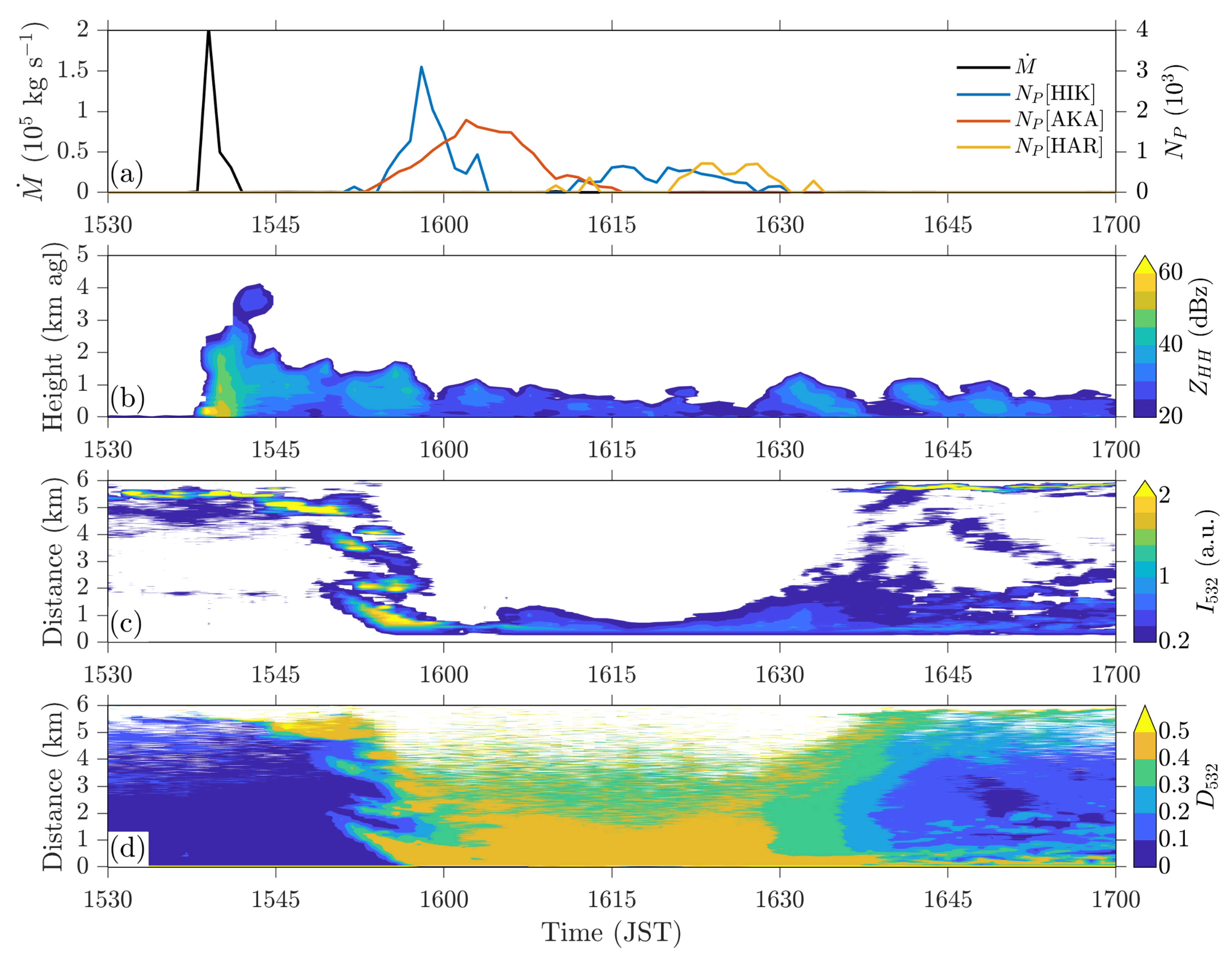
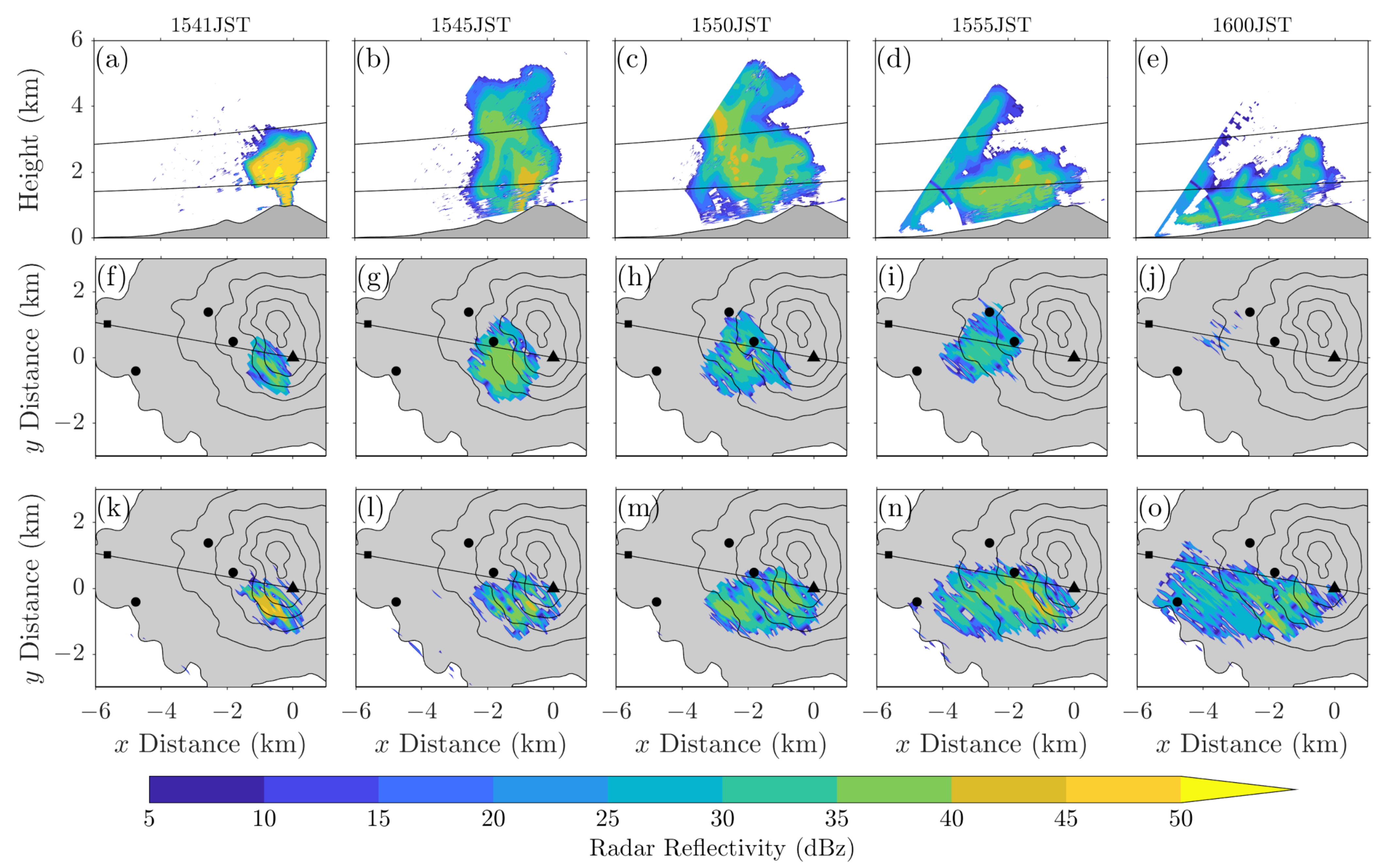
  • Data from the horizontally and vertically scanning radars were used to study the plume generation and initial transport over the volcano.
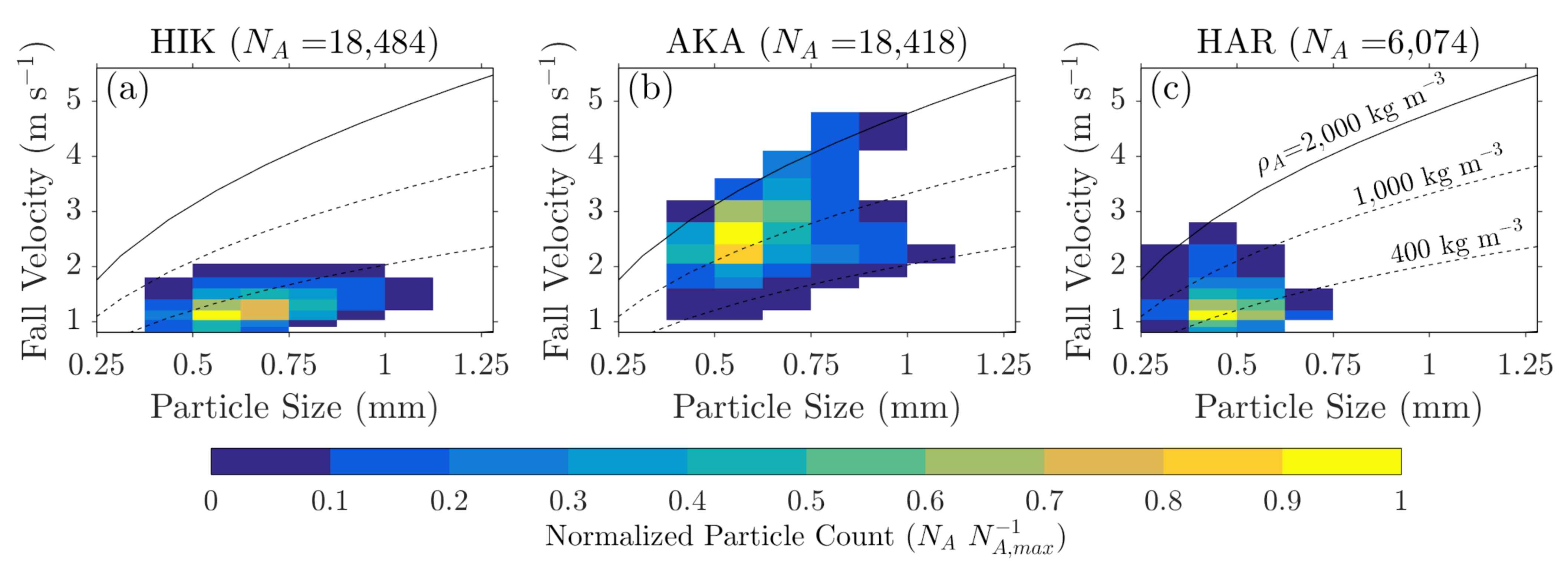
  • Optical disdrometer data revealed significant differences in the sedimentation processes along the main plume axis and along the plume margins.
  • Simulations coupling the WRF and FALL3D models were able to realistically reproduce the observed transport and deposition patterns.
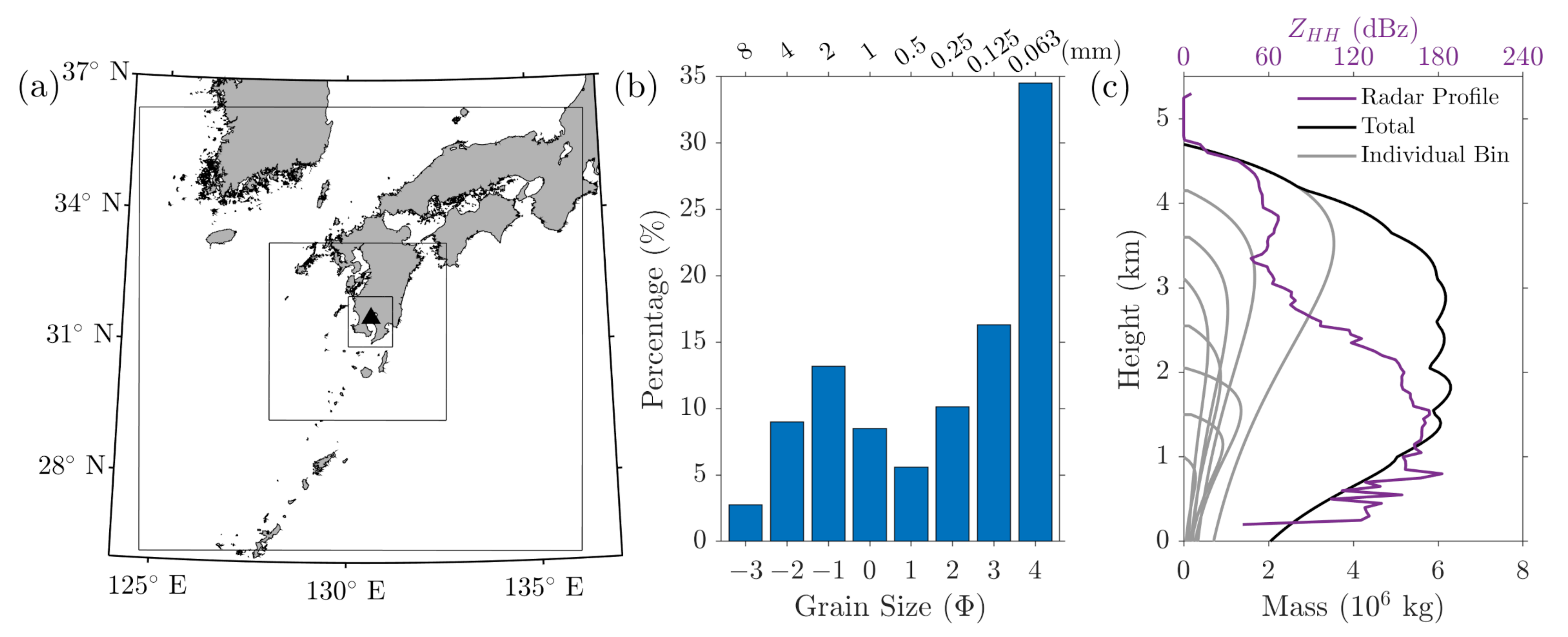
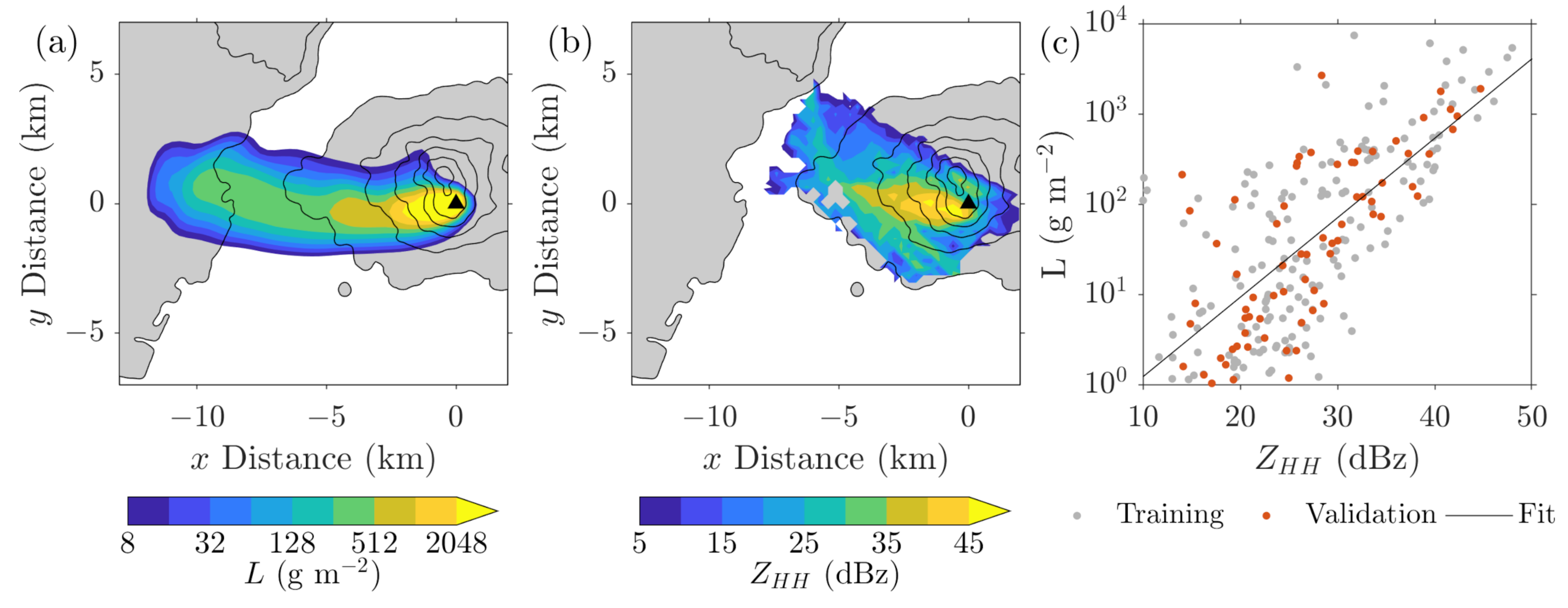
  • Using linear regression the maximum of the radar reflectivity data (with respect to both time and height) was linked to the logarithm of the simulated total accumulated deposit.
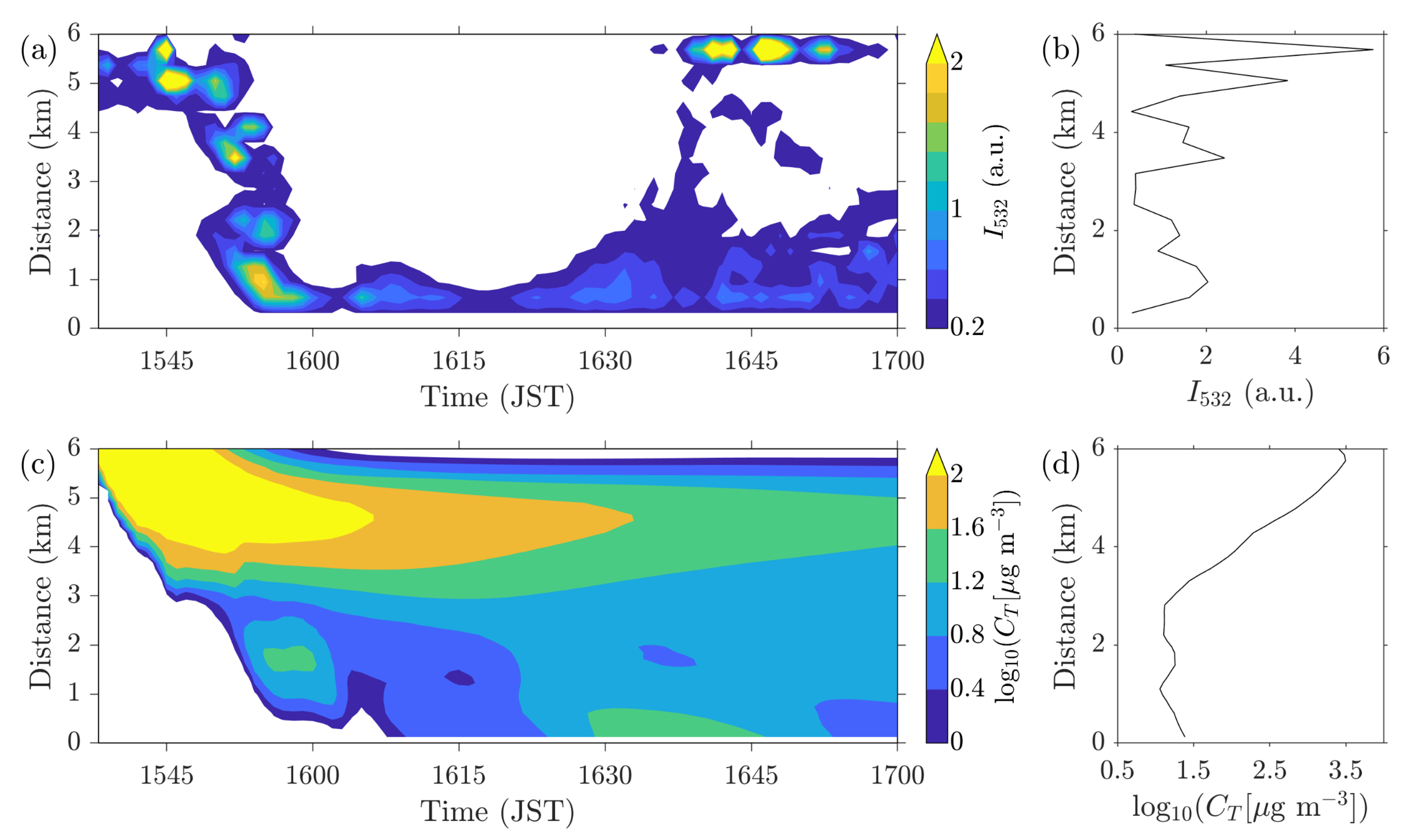
  • A possible link between the maximum lidar backscatter intensity (with respect to time) and the maximum of the airborne tephra concentration logarithm was explored.

Author Contributions

Conceptualization, A.P.P., A.S., H.N. and M.I.; methodology, A.P.P. and A.S.; software, A.P.P.; validation, A.P.P.; formal analysis, A.P.P.; investigation, A.P.P.; resources, H.N. and M.I.; data curation, A.P.P., A.S. and H.N.; writing—original draft preparation, A.P.P.; writing—review and editing, A.P.P., A.S., H.N. and M.I.; visualization, A.P.P.; supervision, M.I.; project administration, M.I.; funding acquisition, M.I. All authors have read and agreed to the published version of the manuscript.

Funding

This research was funded by Integrated Program for the Next Generation Volcano Research and Human Resource Management project, funded by the Japan Ministry of Education, Culture, Sports, Science and Technology (MEXT).

Institutional Review Board Statement

Not applicable.

Informed Consent Statement

Not applicable.

Data Availability Statement

The data presented in this study are available on request from the corresponding author.

Acknowledgments

All simulations were carried out on the Kyoto University supercomputer system. The authors would like to thank 3 anonymous reviewers for their supportive and insightful comments that helped improved the manuscript.

Conflicts of Interest

The authors declare no conflict of interest.

References

  1. Wilson, T.M.; Stewart, C.; Sword-Daniels, V.; Leonard, G.S.; Johnston, D.M.; Cole, J.W.; Wardman, J.; Wilson, G.; Barnard, S.T. Volcanic ash impacts on critical infrastructure. Phys. Chem. Earth Parts A/B/C 2012, 45, 5–23. [Google Scholar] [CrossRef]
  2. Jenkins, S.F.; Wilson, T.M.; Magill, C.; Miller, V.; Stewart, C.; Blong, R.; Marzocchi, W.; Boulton, M.; Bonadonna, C.; Costa, A. Volcanic Ash Fall Hazard and Risk; Cambridge University Press: Cambridge, UK, 2015; pp. 173–222. [Google Scholar] [CrossRef]
  3. Barclay, J.; Few, R.; Armijos, M.T.; Phillips, J.C.; Pyle, D.M.; Hicks, A.J.; Brown, S.K.; Robertson, R.E.A. Livelihoods, wellbeing and the risk to life during volcanic eruptions. Front. Earth Sci. 2019, 7, 205. [Google Scholar] [CrossRef] [Green Version]
  4. Covey, J.; Horwell, C.J.; Ogawa, R.; Baba, T.; Nishimura, S.; Hagino, M.; Merli, C. Community perceptions of protective practices to prevent ash exposures around Sakurajima volcano, Japan. Int. J. Disaster Risk Reduct. 2020, 2020, 101525. [Google Scholar] [CrossRef]
  5. Iguchi, M.; Nakamichi, H.; Tanaka, H.; Ohta, Y.; Shimizu, A.; Miki, D. Integrated monitoring of volcanic ash and forecasting at Sakurajima volcano, Japan. J. Disaster Res. 2019, 14, 798–809. [Google Scholar] [CrossRef]
  6. Poulidis, A.P.; Takemi, T.; Shimizu, A.; Iguchi, M.; Jenkins, S.F. Statistical analysis of dispersal and deposition patterns of volcanic emissions from Mt. Sakurajima, Japan. Atmos. Environ. 2018, 179, 305–320. [Google Scholar] [CrossRef]
  7. Poulidis, A.P.; Takemi, T.; Iguchi, M. The effect of wind and atmospheric stability on the morphology of volcanic plumes from vulcanian eruptions. J. Geophys. Res. Solid Earth 2019, 124, 8013–8029. [Google Scholar] [CrossRef]
  8. Biass, S.; Todde, A.; Cioni, R.; Pistolesi, M.; Geshi, N.; Bonadonna, C. Potential impacts of tephra fallout from a large-scale explosive eruption at Sakurajima volcano, Japan. Bull. Volcanol. 2017, 79, 73. [Google Scholar] [CrossRef] [Green Version]
  9. Iguchi, M. Method for real-time evaluation of discharge rate of volcanic ash—Case study on intermittent eruptions at the Sakurajima volcano, Japan–. J. Disaster Res. 2016, 11, 4–14. [Google Scholar] [CrossRef]
  10. Marzano, F.S.; Barbieri, S.; Vulpiani, G.; Rose, W.I. Volcanic ash cloud retrieval by ground-based microwave weather radar. IEEE Trans. Geosci. Remote 2006, 44, 3235–3246. [Google Scholar] [CrossRef]
  11. Marzano, F.S.; Marchiotto, S.; Textor, C.; Schneider, D.J. Model-based weather radar remote sensing of explosive volcanic ash eruption. IEEE Geosci. Remote Sens. 2010, 48, 3591–3607. [Google Scholar] [CrossRef]
  12. Maki, M.; Iguchi, M.; Maesaka, T.; Miwa, T.; Tanada, T.; Kozono, T.; Momotani, T.; Yamaji, A.; Kakimoto, I. Preliminary results of weather radar observations of Sakurajima volcanic smoke. J. Disaster Res. 2016, 11, 15–30. [Google Scholar] [CrossRef]
  13. Oishi, S.; Iida, M.; Muranishi, M.; Ogawa, M.; Hapsari, R.I.; Iguchi, M. Mechanism of volcanic tephra falling detected by X-band multi-parameter radar. J. Disaster Res. 2016, 11, 43–52. [Google Scholar] [CrossRef]
  14. Sato, E.; Fukui, K.; Shimbori, T. Aso volcano eruption on 8 October 2016, observed by weather radars. Earth Planets Space 2018, 70, 1–8. [Google Scholar] [CrossRef]
  15. Freret-Lorgeril, V.; Gilchrist, J.; Donnadieu, F.; Jellinek, A.M.; Delanoë, J.; Latchimy, T.; Vinson, J.P.; Caudoux, C.; Peyrin, F.; Hervier, C.; et al. Ash sedimentation by fingering and sediment thermals from wind-affected volcanic plumes. Earth Planet. Sci. Lett. 2020, 534, 116072. [Google Scholar] [CrossRef]
  16. Syarifuddin, M.; Oishi, S.; Nakamichi, H.; Maki, M.; Hapsari, R.I.; Mawandha, H.G.; Aisyah, N.; Basuki, A.; Loeqman, A.; Shimomura, M.; et al. A real-time tephra fallout rate model by a small-compact X-band Multi-Parameter radar. J. Volcanol. Geotherm. Res. 2020, 405, 107040. [Google Scholar] [CrossRef]
  17. Sassen, K.; Zhu, J.; Webley, P.; Dean, K.; Cobb, P. Volcanic ash plume identification using polarization lidar: Augustine eruption, Alaska. Geophys. Res. Lett. 2007, 34. [Google Scholar] [CrossRef]
  18. Ansmann, A.; Tesche, M.; Groß, S.; Freudenthaler, V.; Seifert, P.; Hiebsch, A.; Schmidt, J.; Wandinger, U.; Mattis, I.; Müller, D.; et al. The 16 April 2010 major volcanic ash plume over central Europe: EARLINET lidar and AERONET photometer observations at Leipzig and Munich, Germany. Geophys. Res. Lett. 2010, 37, L13810. [Google Scholar] [CrossRef] [Green Version]
  19. Gross, S.; Freudenthaler, V.; Wiegner, M.; Gasteiger, J.; Geiss, A.; Schnell, F. Dual-wavelength linear depolarization ratio of volcanic aerosols: Lidar measurements of the Eyjafjallajökull plume over Maisach, Germany. Atmos. Environ. 2012, 48, 85–96. [Google Scholar] [CrossRef] [Green Version]
  20. Poulidis, A.P.; Takemi, T.; Iguchi, M. Experimental high-resolution forecasting of volcanic ash hazard at Sakurajima, Japan. J. Disaster Res. 2019, 14, 786–797. [Google Scholar] [CrossRef] [Green Version]
  21. Poulidis, A.P.; Iguchi, M. Model sensitivities in the case of high-resolution Eulerian simulations of local tephra transport and deposition. Atmos. Res. 2021, 247, 105136. [Google Scholar] [CrossRef]
  22. Freret-Lorgeril, V.; Donnadieu, F.; Eychenne, J.; Soriaux, C.; Latchimy, T. In situ terminal settling velocity measurements at Stromboli volcano: Input from physical characterization of ash. J. Volcanol. Geotherm. Res. 2019, 374, 62–79. [Google Scholar] [CrossRef] [Green Version]
  23. Kozono, T.; Iguchi, M.; Miwa, T.; Maki, M.; Maesaka, T.; Miki, D. Characteristics of tephra fall from eruptions at Sakurajima volcano, revealed by optical disdrometer measurements. Bull. Volcanol. 2019, 81, 5–48. [Google Scholar] [CrossRef]
  24. Tanaka, H.L.; Iguchi, M. Numerical simulations of volcanic ash plume dispersal for Sakura-Jima using real-time emission rate estimation. J. Disaster Res. 2019, 14, 160–172. [Google Scholar] [CrossRef]
  25. Graf, H.F.; Herzog, M.; Oberhuber, J.M.; Textor, C. Effect of environmental conditions on volcanic plume rise. J. Geophys. Res. Atmos. 1999, 104, 24309–24320. [Google Scholar] [CrossRef] [Green Version]
  26. Montopoli, M.; Vulpiani, G.; Cimini, D.; Picciotti, E.; Marzano, F.S. Interpretation of observed microwave signatures from ground dual polarization radar and space multi-frequency radiometer for the 2011 Grimsvotn volcanic eruption. Atmos. Meas. Tech. 2014, 7, 537. [Google Scholar] [CrossRef] [Green Version]
  27. Folch, A. A review of tephra transport and dispersal models: Evolution, current status, and future perspectives. J. Volcanol. Geotherm. Res. 2012, 235, 96–115. [Google Scholar] [CrossRef]
  28. Folch, A.; Mingari, L.; Guitierrez, N.; Hanzich, M.; Macedonio, G.; Costa, A. FALL3D-8.0: A computational model for atmospheric transport and deposition of particles, aerosols and radionuclides—Part 1: Model physics and numerics. Geosci. Model Dev. 2020, 13, 1431–1458. [Google Scholar] [CrossRef] [Green Version]
  29. Prata, A.T.; Mingari, L.; Folch, A.; Macedonio, G.; Costa, A. FALL3D-8.0: A computational model for atmospheric transport and deposition of particles, aerosols and radionuclides–Part 2: Model applications. Geosci. Model Dev. Discuss. 2020, 1–40, in review. [Google Scholar] [CrossRef]
  30. Degruyter, W.; Bonadonna, C. Improving on mass flow rate estimates of volcanic eruptions. Geophys. Res. Lett. 2012, 39. [Google Scholar] [CrossRef] [Green Version]
  31. Poret, M.; Corradini, S.; Merucci, L.; Costa, A.; Andronico, D.; Montopoli, M.; Vulpiani, G.; Freret-Lorgeril, V. Reconstructing volcanic plume evolution integrating satellite and ground-based data: Application to the 23 November 2013 Etna eruption. Atmos. Chem. Phys. 2018, 18, 4695. [Google Scholar] [CrossRef] [Green Version]
  32. Tokay, A.; Wolff, D.B.; Petersen, W.A. Evaluation of the new version of the laser-optical disdrometer, OTT Parsivel2. J. Atmos. Ocean. Technol. 2014, 31, 1276–1288. [Google Scholar] [CrossRef]
  33. Yuter, S.E.; Kingsmill, D.E.; Nance, L.B.; Löffler-Mang, M. Observations of precipitation size and fall speed characteristics within coexisting rain and wet snow. J. Appl. Meteorol. Clim. 2006, 45, 1450–1464. [Google Scholar] [CrossRef] [Green Version]
  34. Bohren, C.F.; Huffman, D.R. Absorption and Scattering of Light by Small Particles; John Wiley & Sons: Hoboken, NJ, USA, 2008. [Google Scholar] [CrossRef] [Green Version]
  35. Sassen, K. Polarization in lidar. In Lidar; Weitkamp, C., Ed.; Springer: New York, NY, USA, 2005; pp. 19–42. [Google Scholar]
  36. Bagheri, G.; Rossi, E.; Biass, S.; Bonadonna, C. Timing and nature of volcanic particle clusters based on field and numerical investigations. J. Volcanol. Geotherm. Res. 2016, 327, 520–530. [Google Scholar] [CrossRef] [Green Version]
  37. Gabellini, P.; Rossi, E.; Bonadonna, C.; Pistolesi, M.; Bagheri, G.; Cioni, R. Physical and aerodynamic characterization of particle clusters at Sakurajima Volcano (Japan). Front. Earth Sci. 2020, 8, 575874. [Google Scholar] [CrossRef]
  38. Suzuki, T. A theoretical model for dispersion of tephra. In Arc Volcanism: Physics and Tectonics; Shimozuru, D., Yokoyama, I., Eds.; Terra Scientific Publishing Company (TERRAPUB): Tokyo, Japan, 1983; pp. 95–113. [Google Scholar]
  39. Ernst, G.G.J.; Davis, J.P.; Sparks, R.S.J. Bifurcation of volcanic plumes in a crosswind. Bull. Volcanol. 1994, 56, 159–169. [Google Scholar] [CrossRef]
  40. Manzella, I.; Bonadonna, C.; Phillips, J.C.; Monnard, H. The role of gravitational instabilities in deposition of volcanic ash. Geology 2015, 43, 211–214. [Google Scholar] [CrossRef] [Green Version]
  41. Skamarock, W.C.; Klemp, J.B.; Dudhia, J.; Gill, D.O.; Liu, Z.; Berner, J.; Wang, W.; Power, J.G.; Duda, M.G.; Barker, D.M.; et al. A Model Description of the Advanced Research WRF Model Version 4 (No. NCAR/TN-556+STR); Technical Report; National Center for Atmoshperic Research: Boulder, CO, USA, 2019. [Google Scholar] [CrossRef]
  42. Marti, A.; Folch, A. Volcanic ash modeling with the NMMB-MONARCH-ASH model: Quantification of offline modeling errors. Atmos. Chem. Phys. 2018, 18, 4019–4038. [Google Scholar] [CrossRef] [Green Version]
  43. Takemi, T.; Ito, R. Benefits of high-resolution downscaling experiments for assessing strong wind hazard at local scales in complex terrain: A case study of Typhoon Songda (2004). Prog. Earth Planet. Sci. 2020, 7, 1–16. [Google Scholar] [CrossRef]
  44. Hersbach, H.; Bell, B.; Berrisford, P.; Hirahara, S.; Horányi, A.; Muñoz-Sabater, J.; Nicolas, J.; Peubey, C.; Radu, R.; Schepers, D.; et al. The ERA5 global reanalysis. Q. J. R. Meteorol. Soc. 2020, 146, 1999–2049. [Google Scholar] [CrossRef]
  45. Osores, M.S.; Ruiz, J.; Folch, A.; Collini, E. Volcanic ash forecast using ensemble-based data assimilation: The Ensemble Transform Kalman Filter coupled with FALL3D-7.2 model (ETKF-FALL3D, version 1.0). Geosci. Model Dev. 2019. [Google Scholar] [CrossRef]
  46. Parra, R. Influence of spatial resolution in modeling the dispersion of volcanic ash in Ecuador. WIT Trans. Ecol. Environ. 2019, 236, 67–78. [Google Scholar] [CrossRef] [Green Version]
  47. Folch, A.; Jorba, O.; Viramonte, J. Volcanic ash forecast-application to the May 2008 Chaitén eruption. Nat. Hazards Earth Syst. Sci 2008, 8, 927–940. [Google Scholar] [CrossRef]
  48. Corradini, S.; Merucci, L.; Folch, A. Volcanic ash cloud properties: Comparison between MODIS satellite retrievals and FALL3D transport model. IEEE Geosci. Remote Sens. Lett. 2010, 8, 248–252. [Google Scholar] [CrossRef]
  49. Poret, M.; Costa, A.; Folch, A.; Martí, A. Modelling tephra dispersal and ash aggregation: The 26th April 1979 eruption, La Soufrière St. Vincent. J. Volcanol. Geotherm. Res. 2017, 347, 207–220. [Google Scholar] [CrossRef]
  50. Shin, H.H.; Hong, S.Y. Representation of the subgrid-scale turbulent transport in convective boundary layers at gray-zone resolutions. Mon. Weather Rev. 2015, 143, 250–271. [Google Scholar] [CrossRef]
  51. Wyngaard, J.C. Toward numerical modeling in the “Terra Incognita”. J. Atmos. Sci. 2004, 61, 1816–1826. [Google Scholar] [CrossRef]
  52. Kessler, E. On the distribution and continuity of water substance in atmospheric circulations. In On the Distribution and Continuity of Water Substance in Atmospheric Circulations; American Meteorological Society: Boston, MA, USA, 1969; pp. 1–84. [Google Scholar] [CrossRef]
  53. Iacono, M.J.; Delamere, J.S.; Mlawer, E.J.; Shephard, M.W.; Clough, S.A.; Collins, W.D. Radiative forcing by long-lived greenhouse gases: Calculations with the AER radiative transfer models. J. Geophys. Res. Atmos. 2008, 113, D13. [Google Scholar] [CrossRef]
  54. Jiménez, P.A.; Dudhia, J.; González-Rouco, J.F.; Navarro, J.; Montávez, J.P.; García-Bustamante, E. A revised scheme for the WRF surface layer formulation. Mon. Weather Rev. 2012, 140, 898–918. [Google Scholar] [CrossRef] [Green Version]
  55. Dudhia, J. A multi-layer soil temperature model for MM5. In Preprints, The Sixth PSU/NCAR Mesoscale Model Users’ Workshop; National Center for Atmospheric Research: Boulder, CO, USA, 1996; pp. 22–24. [Google Scholar]
  56. Costa, A.; Pioli, L.; Bonadonna, C. Assessing tephra total grain-size distribution: Insights from field data analysis. Earth Planet. Sci. Lett. 2016, 443, 90–107. [Google Scholar] [CrossRef]
  57. Ganser, G.H. A rational approach to drag prediction of spherical and nonspherical particles. Powder Technol. 1993, 77, 143–152. [Google Scholar] [CrossRef]
  58. Sulpizio, R.; Folch, A.; Costa, A.; Scaini, C.; Dellino, P. Hazard assessment of far-range volcanic ash dispersal from a violent Strombolian eruption at Somma-Vesuvius volcano, Naples, Italy: Implications on civil aviation. Bull. Volcanol. 2012, 74, 2205–2218. [Google Scholar] [CrossRef]
  59. Clarke, A.B.; Voight, B.; Neri, A.; Macedonio, G. Transient dynamics of vulcanian explosions and column collapse. Nature 2002, 415, 897–901. [Google Scholar] [CrossRef] [PubMed]
  60. Folch, A.; Costa, A.; Macedonio, G. FPLUME-1.0: An integral volcanic plume model accounting for ash aggregation. Geosci. Model Dev. 2016, 9, 431–450. [Google Scholar] [CrossRef] [Green Version]
  61. Scollo, S.; Bonadonna, C.; Manzella, I. Settling-driven gravitational instabilities associated with volcanic clouds: New insights from experimental investigations. Bull. Volcanol. 2017, 79, 39. [Google Scholar] [CrossRef] [Green Version]
  62. Gilbert, J.S.; Lane, S.J. The origin of accretionary lapilli. Bull. Volcanol. 1994, 56, 398–411. [Google Scholar] [CrossRef]
  63. Efron, B. Estimating the error rate of a prediction rule: Improvement on cross-validation. J. Am. Stat. Assoc. 1982, 78, 316–331. [Google Scholar] [CrossRef]
  64. Costa, A.; Folch, A.; Macedonio, G. A model for wet aggregation of ash particles in volcanic plumes and clouds: 1. Theoretical formulation. J. Geophys. Res. Solid Earth 2010, 115. [Google Scholar] [CrossRef]
  65. Folch, A.; Costa, A.; Durant, A.; Macedonio, G. A model for wet aggregation of ash particles in volcanic plumes and clouds: 2. Model application. J. Geophys. Res. Solid Earth 2010, 115. [Google Scholar] [CrossRef]
  66. Poulidis, A.P.; Takemi, T.; Iguchi, M.; Renfrew, I.A. Orographic effects on the transport and deposition of volcanic ash: A case study of Mount Sakurajima, Japan. J. Geophys. Res. Atmos. 2017, 122, 9332–9350. [Google Scholar] [CrossRef]
Figure 1. (a) Location of Sakurajima in Japan. (b) Topographic map of the surrounding area overlaid with with locations of observational equipment used in this study.
Atmosphere 12 00104 g001
Figure 2. (a) Mass flow rate estimate ( M . ; left-hand axis, black line) and number of observed particles ( N P ; coloured lines shown at the right-hand axis). (b) Radar reflectivity ( Z H H ) over the vent. (c) Lidar backscatter intensity ( I 532 ) shown in arbitrary units. (d) Lidar depolarisation ratio ( D 532 ). Note that the distance shown in Panels c and d is the distance from the receiver pointing towards the volcanic vent.
Atmosphere 12 00104 g002
Figure 3. (ae) Radar reflectivity data from the vertically-scanning Sakurajima Volcanological Observatory (SVO) radar. (fo) Radar reflectivity data from the Hirakawa radar scanning horizontally at an elevation of: (fj) 10° and (ko) 5°. The black lines at Panels (ae) indicate the two elevations scanned by the Hirakawa radar, while the black line on Panels (fo) indicates the vertical radar scanning cross-section. Markers follow Figure 1. Note that both x and y distances are shown from the volcanic vent.
Atmosphere 12 00104 g003
Figure 4. Disdrometer observations of particle size against particle fall velocity for: (a) Hikinohira (HIK), (b) Akamizu (AKA), and (c) Haruta (HAR). Cell colour shows the normalised particle count, while the three lines show theoretical values for different particle densities (400, 1000, and 2000 kg m−3) based on Reference [38].
Atmosphere 12 00104 g004
Figure 5. (a) Placement of the WRF domains. (b) Total grain size distribution used in the study. (c) Mass distribution along the plume profile. The total mass is shown in black, the individual distribution for each grain size is shown in gray, and the accumulated radar reflectivity between 1538–1543 JST is shown in purple using the upper x axis.
Atmosphere 12 00104 g005
Figure 6. Total simulated load at the end of the simulation (shaded) overlaid by the contour enclosing total airborne tephra concentration ≥100 μ g m−3 at: (a) 1543, (b) 1553, (c) 1608, (d) 1623, (e) 1638, and (f) 1658 JST. Disdrometer locations are shown using a circle marker, with the observed value on the left side and the right side left transparent. Note that both x and y distances are shown from the volcanic vent.
Atmosphere 12 00104 g006
Figure 7. (a) Total simulated load. (b) Maximum observed radar reflectivity with respect to time. (c) Scatter plot of radar reflectivity against total simulated load. The points in gray were used to calculate the fitting parameters, while the points shown in orange were used for the error analysis. Note that both x and y distances in Panels a and b are shown from the volcanic vent.
Atmosphere 12 00104 g007
Figure 8. (a) Lidar backscatter intensity resampled for comparison against model data. (b) Maximum backscatter intensity with distance. (c) Modelled airborne tephra concentration along the lidar observation line. (d) Logarithm of the maximum modelled tephra concentration.
Atmosphere 12 00104 g008
Publisher’s Note: MDPI stays neutral with regard to jurisdictional claims in published maps and institutional affiliations.

