Public Health Considerations for PM10 in a High-Pollution Megacity: Influences of Atmospheric Condition and Land Coverage


1
Grupo de Investigación en Ingeniería Ambiental GIIAUD, Facultad del Medio Ambiente y Recursos Naturales, Universidad Distrital Francisco José de Caldas, Carrera 5 Este #15-82, E-111711 Bogotá, Colombia
2
Grupo de Enxeñaría da Auga e do Medio Ambiente (GEAMA), Campus de Elviña, Universidade da Coruña (UdC), s/n, 15071 A Coruña, Spain
3
Centro Lasallista de Investigación y Modelación Ambiental CLIMA, Universidad de La Salle, Carrera 2 #10-70, E-111711 Bogotá, Colombia
*
Author to whom correspondence should be addressed.
Atmosphere 2021, 12(1), 118; https://0-doi-org.brum.beds.ac.uk/10.3390/atmos12010118
Submission received: 17 December 2020
/
Revised: 2 January 2021
/
Accepted: 6 January 2021
/
Published: 15 January 2021
(This article belongs to the Section Air Quality and Human Health)
Abstract
:This paper analyzes the PM10 concentrations and influences of atmospheric condition (AC) and land coverage (LC) on a high-pollution megacity (Bogota, Colombia) from a public health viewpoint. Information of monitoring stations equipped with measuring devices for PM10/temperature/solar-radiation/wind-speed were used. The research period lasted eight years (2007–2014). AC and LC were determined after comparing daily PM10 concentrations (DPM10) to reference limits published by the World Health Organization (WHO). ARIMA models for DPM10 were also developed. The results indicated that urban sectors with lower atmospheric instability (AI) had a 2.85% increase in daily mortality (DM) in relation to sectors with greater AI. In these sectors of lower AI, impervious LC predominated, instead of vegetated LC. An ARIMA analysis revealed that a greater extent of impervious LC around a station led to a greater effect on previous days’ DPM10 concentrations. Extreme PM10 episodes persisted for up to two days. Extreme pollution episodes were probably also preceded by low mixing-layer heights (between 722–1085 m). The findings showed a 13.0% increase in WHO standard excesses (PE) for each 10 µg/m3 increase in DPM10, and a 0.313% increase in DM for each 10% increase in PE. The observed average reduction of 14.8% in DPM10 (−0.79% in DM) was probably due to 40% restriction of the traffic at peak hours.
1. Introduction
The increase of respiratory and cardiovascular diseases in children and elderly generated by urban air pollution is strongly related to an increase of particulate material (PM) concentrations [1,2]. The impacts of PM on human health are associated with a reduction of the cardiopulmonary functions and increased mortality from cardiovascular disease, the occurrence of asthma in children, and cancer risk [3,4]. Some researchers have reported that diseases such as bronchitis and chronic asthma are directly correlated with PM pollution [5]. In a European study on atmospheric pollution and its effects on public health, it was reported that an increase of 50 μg/m3 in PM10 concentration could cause an increase of 2.10% in the daily mortality (DM) of 15 cities in Western Europe [6]. In Chinese megacities (Guangzhou, Wuhan, and Chongqing) and with support from the U.S. Environmental Protection Agency (U.S. EPA), research was conducted on the effects of air pollution on respiratory health. After several years of follow-up, it was determined that PM10 concentration was directly related to the rate of infantile pulmonary dysfunction [7].
In Colombia, air pollution has been associated with morbidity and mortality outcomes. In a recent study, rates of emergency department visits for respiratory and circulatory diseases in four of the five major Colombian cities during 2011–2014 were linked with gas pollutants and PM concentrations. An increase in 10 µg/m3 of PM10 or 5 µg/m3 of PM2.5 was associated with an increase of 8.0% in respiratory diseases in children less than 10 years old and 5.0% increase in cardiovascular diseases in the elderly [8]. For Bogota, a time series study in the 1998–2006 period observed an increase of 0.71% of mortality for all causes and 1.43% for respiratory outcomes for an increase of 10 µg/m3 of PM10 [9].
The urban increase of PM is principally related to growth in the number of vehicles and the grouping of industrial activities [10]. Because of this, many Latin American countries have resolved to strengthen urban PM monitoring to regulate this air pollutant [11,12]. Hence, the analysis of a likely relationship between urban PM and the dominant atmospheric condition (AC) becomes crucial from a perspective of public health. The land coverage (LC) typologies of the research site must be known in order to perform such an analysis. For example, some researchers observed that the transport and distribution of PM depended considerably on AC and LC [13,14].
Studies have reported that AC plays a significant role in the PM10 dispersion and transport, being significantly related to vertical temperature variation (thermal gradient) and wind speed [15,16]. The latter variable also depends on the LC characteristics [17,18]. Related to AC influence, some researchers reported for Seoul (Korea) that under extreme atmospheric stability (AS) conditions the PM10 concentrations tended to increase significantly (PM10 > 100 μg/m3) [19]. Studies in Milan (Italy) also reported an increase of 13% in PM10 concentrations under dominant conditions of nighttime AS, despite a decrease in the emission sources (domestic heating, traffic, and industries) [20].
On the other hand, studies in urban sectors have also described an important influence of LC on PM10 concentrations. For example, some researchers stated that the existence of trees in Wuhan (China) decreased PM10 concentrations between 7–15% [14]. Similarly, other studies observed a decrease of total PM (<100 μm) in Shanghai (China) by 30% [21]. Urban LC with trees functions as an effective remover of particulate and gaseous air pollutants [22,23]. Though, the mineral sediment emitted by bare soils was recognized as the air deterioration source in Central Europe cities (e.g., Zurich and Berlin) [24,25]. Some researchers also observed in Granada (Spain) that more than 50% of PM10 belonged to mineral sediment resuspended from urban roads and bare lands during dry periods [26]. Other studies reported in Lens (France) that 13% of average annual PM10 could be generated from bare lands (sources of mineral sediment) [27]. Some researchers compared the PM elimination capacity on different surfaces in Beijing [28]. These researchers observed that urban woodland surface achieved the best PM elimination capacity due to its comparatively low resuspension degree. They also noted that the PM elimination capacity of waterbodies was higher than that of bare soils due its lower resuspension degree.
This research was conducted in a highly-polluted Latin American megacity (population in 2019:10.7 million). Bogota (Colombia) is in a very large inter-montane valley in the eastern Andes mountain range (04°36′35″ N–74°04′54″ W) at an average altitude of 2600 m above sea level (masl). Its climate of tropical mountain is marked by large temperature variations (maximum hourly variation = 12 °C). According to some studies, conditions of daytime atmospheric instability (AI) are recorded due to the increase of solar radiation up to midday and early afternoon [29]. During nighttime, wind speeds are very low, indicating stable and neutral atmospheric conditions. In Latin America, Bogota has the third highest PM pollution degree and the highest population density (26,000/km2) [30]. Therefore, interactions among the degree of PM10 pollution, climate conditions, and the physical characteristics of the city provided the impetus for the present research. Also, few studies have assessed the PM10 behavior in megacities in developing countries with comparable characteristics regarding pollution and altitude.
This paper aims to analyze, from a public health viewpoint, the PM10 concentrations and influences of AC and LC on this high-pollution megacity. The research was developed from hourly PM10 information between the years 2007–2014 from monitoring stations placed throughout the city. This study will increase our knowledge about: (1) The status of air quality for the Latin American city with the third highest atmospheric pollution as compared to the World Health Organization Guidelines; (2) the trend of PM10 concentrations in megacities in developing countries, in this case, under high-altitude climate conditions; and (3) the influences of AC and LC on PM10 concentrations in megacities.
2. Materials and Methods
2.1. Study Sites
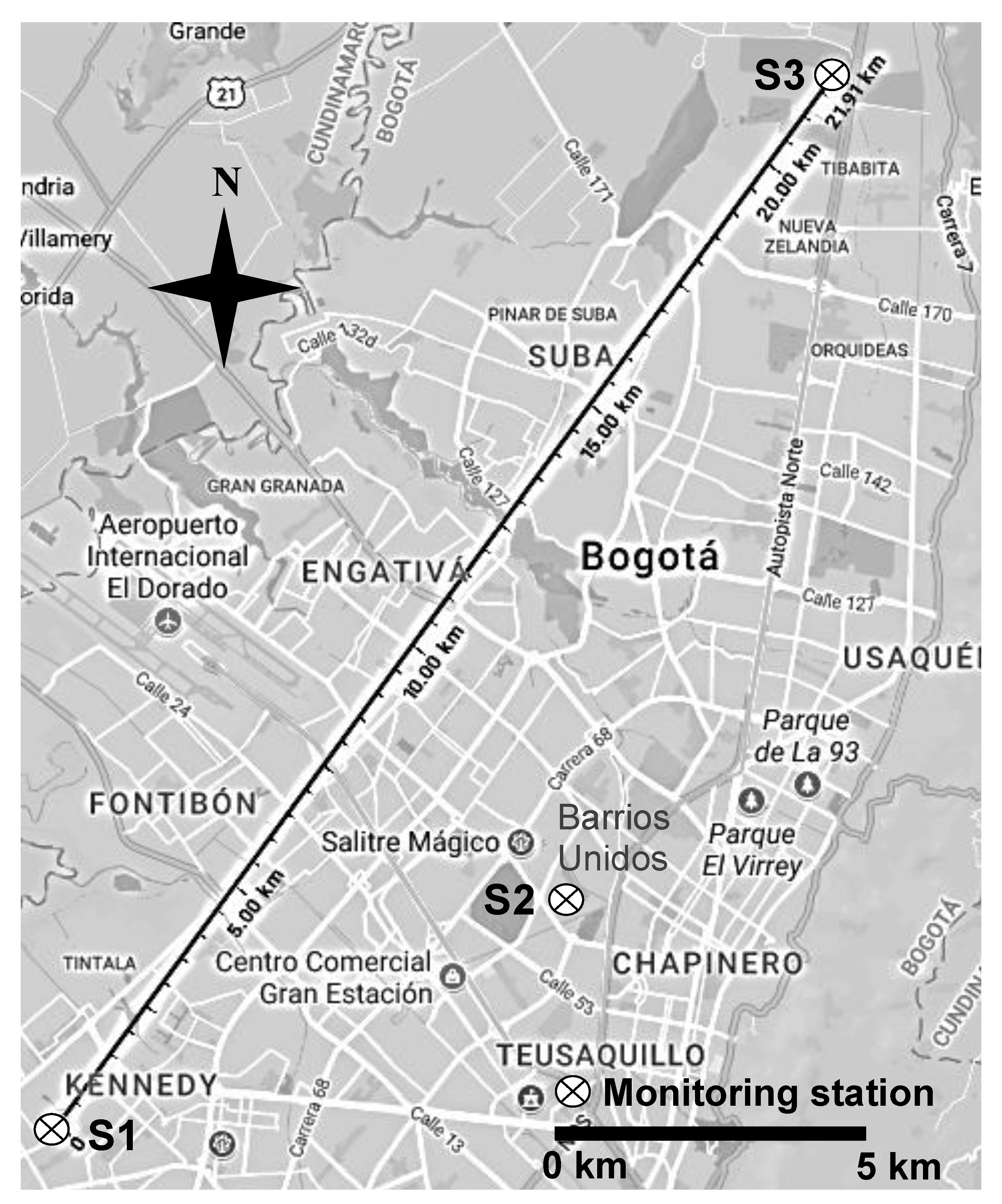
Three monitoring stations were positioned in sectors Kennedy (S1), Barrios Unidos (S2), and Suba (S3) in Bogota, Colombia. On average, tropical mountainous climates were characterized at these research sites during the research period by showing a daily temperature between 13.3–14.3 °C and wide temperature variations (hourly variation between 7.2–19 °C). Table 1 displays the main characteristics of the sectors of influence for each station. All three stations were prepared with PM10 measuring devices, as well as devices to measure temperature, solar radiation (RD), and wind speed (WS) and direction. All stations were of background type. The stations considered in this research covered 21.9 km of the city, compared to the 33 km that it has from north to south (Figure 1). The stations were placed in sites with altitudes between 2577–2580 masl. During the research period in Bogota (1 January 2007–31 December 2014), there was a restriction on vehicular movement because of traffic congestion from Monday to Friday. This restriction, “pico y placa”, prevented 40% of the city’s passenger vehicles (between 425,000–817,000) from circulating between 6–9 a.m. and 3–7 p.m. [31]. Lastly, a PM10 emissions inventory in the city showed that by 2014, the contributions were as follows: Mobile sources = 53.8%, industrial fixed sources = 39.3%, commercial fixed sources = 4.74%, and forest fires = 2.22% [31].
2.2. PM10 Sampling
The research period lasted eight years. This time interval was selected because the sectors surrounding the stations displayed no significant changes in LC (impervious/vegetated/nonvegetated/waterbodies; see Table 1). Thus, during the research period, the possible effects of the LC variation on AC (vertical gradient of temperature and WS) in each sampling site were minimized. The hourly PM10 sampling was performed with continuous beta-ray attenuation equipment (BAM/1020, Met One Instruments, Grants Pass, OR, USA). The equipment used had a constant flow rate of 16.7 L/min. The lowest detection limit of the equipment was 3.6 µg/m3 and 1.0 µg/m3 for hourly and daily periods, respectively. Resolution in the measurement was 0.24 µg in a range of 1 mg. The precision was ± 8% and ± 2% for hourly and daily periods, respectively. The research protocol followed the recommendations set forth by U.S. Environmental Protection Agency in EPA/625/R-96/010a-IO-1.2 [32].
2.3. AC and LC Analysis
AC was determined at each station using the methodologies of Gifford, Turner, and Pasquill with hourly information for RD and WS [33,34,35]. We analyzed the dominant AC according to its hourly frequency following the methodology proposed by Chambers et al. [18]. Non-normal distribution of AC data was calculated with Shapiro-Wilk test (p-values < 0.001; df = 24) [36]. A Kruskal-Wallis test [36] to evaluate the differences in hourly frequency between stations was used (df = 24, per station). Quantitative scale developed by Zafra et al. to classify AC was used in this research [17]. This quantitative scale assigned values between 1 and 6 to classify AC between stable and very unstable, respectively.
Additionally, we studied the average variation (hourly and daily) of the mixing-layer height (MLH) in Bogota from information provided by the Institute of Hydrology, Meteorology, and Environmental Studies (IDEAM) of Colombia. This information was verified from studies carried out in Bogota by Nedbor-Gross et al., Reboredo et al., and Kumar and Rojas [37,38,39]. These studies used the Weather Research and Forecasting Model (WRF). Finally, Spearman’s coefficient [36] was used to evaluate the association between MLH, and RD and WS. Linear regression models [36] were also developed between these variables.
To evaluate the LC type around each station, we drew on satellite images a box of 10,240,000 m2 (diagonals of 3200 m), and whose center was located on each station (QuickBird satellite of DigitalGlobe Inc., New York, NY, USA, 2.0-m resolution). Moreover, to evaluate the spatial variation per LC type, boxes of different lengths in terms of diagonals were plotted for each station (100/200/400/800/1600/3200 m). Previous studies on air quality and LC were taken as procedural guides [17,23]. Four types of LC were considered in this research: impervious = roofs/pavements/footpaths; vegetated = trees/grasslands; nonvegetated = bare land; and waterbodies = rivers/lakes/wetlands. During the selected PM10 monitoring period there was no LC variation.
2.4. Air Quality Standards Analysis
The selected standards to assess air quality in the research areas were Colombian Resolution No. 610/2010 and WHO Air Quality Guidelines [40,41]. These standards established the following maximum permissible levels for PM10:100 and 50 µg/m3 for a 24-h exposure time. The exceedance frequencies of these maximum permissible levels during the whole research period were analyzed for daily and monthly time scales. According to the daily PM10 concentrations (DMP10), monthly quartiles (Q) were established to assess the public health risk in relation to the reference legislation. Thus, the average daily concentrations were calculated for each month and later the months were organized in order of precedence according to their PM10 concentrations. In this research, Q1 quartile was assigned to the three months that exhibited the highest PM10 concentration (greatest public health risk). The quartiles Q2, Q3, and Q4 were assigned in groups of three months according to the order of precedence for PM10 concentration. The Q4 quartile was assigned to the three months of lowest PM10 concentration (lowest public health risk).
2.5. DM Analysis
The increase in DM associated with PM10 for the predominant LC types in the research areas was calculated. This calculation was based on the guidelines established by the study of Blanco-Becerra et al. in Bogota and WHO [9,41]. The results of studies at global level suggested that the public health risks associated with short-term exposures to PM10 were probably similar in cities in developed and developing countries, with an increase in DM around 0.50% for each increase of 10 µg/m3 in DPM10 [41]. Blanco-Becerra et al. observed in Bogota an increase of 0.71% in DM for each increase of 10 µg/m3 in DPM10 [9]. Thus, in our study we assumed an increase in DM of 0.71%. These increases in DM were calculated from the maximum 24-h limit for PM10 established by WHO (50 µg/m3). We also compared the increase in DM from the monthly classification proposed by quartiles to study the exposure risk to PM10. During all previous analyses, the influence of AC was also considered. Non-normal distribution of DM data was calculated with Shapiro-Wilk test (p-values < 0.039) [36]. Finally, Spearman’s coefficient [36] was used to study the association between DPM10 and the excess percentage (PE) relative to the daily WHO limit. This coefficient was also used to evaluate the association between PE and DM. Linear regression models [36] were also developed between these variables.
2.6. PM10 Information Analysis
Hourly variation in PM10 concentrations for all stations was studied from average values for the whole research period (n = 24, per station). DPM10 variation was studied from the 24-h moving average [36]. Non-normal distribution of PM10 data was calculated with Shapiro-Wilk test (p-values < 0.048) [36]. A Spearman’s correlation analysis [36] to study relations in the hourly and daily PM10 concentration between stations was performed. Moreover, the variation of PM10 concentrations at each station was assessed using standard deviation (SD) [36]. All statistical analyses were carried out using IBM-SPSS V.21® software.
A graphical contrast between the hourly variation of average PM10 concentrations and average AC was performed to evaluate the influence of the PM10 emission cycles from industries and motor vehicles across the whole research area. A Spearman’s correlation analysis [36] was also used to analyze possible relationships between these variables. Hourly and daily PM10 of stations situated in sectors with mainly impervious LC (S1) was compared with the PM10 of stations situated in sectors with mainly vegetated LC (S3). The previous analysis also considered the dominant AC in relation to the LC type.
The average difference in DPM10 was determined between the following periods: (1) Monday and Friday, and (2) Saturday; to evaluate the effect of vehicle traffic restriction from Monday to Friday (between 6–9 a.m. and 3–7 p.m.) on PM10 concentrations during the whole research period. This analysis was carried out from the following considerations: (1) The restriction from Monday to Friday was mainly for private vehicles. On average, this vehicle category represented during the research period 68% of the total number of vehicles in Bogota [31]. (2) We assume a uniform distribution in the industrial and commercial activity of Bogota between Monday and Saturday. The weekly hours worked per worker in Colombia during the research period were between 48.3–49.0 (between Monday and Saturday 8.11 h per day). The weekly average for the member countries of the Organization for Economic Co-operation and Development (OECD) during this same period was 38.5 h [42]. (3) Mobile sources contributed during the research period between 55.0–56.5% of PM10 in Bogota [31]. The effect of this measure by traffic congestion in relation to AC and LC was also studied in each station.
We also developed Autoregressive Integrated Moving Average (ARIMA) models to evaluate the variation of PM10 concentrations in relation to AC and LC. Hourly PM10 information was added each day to the analysis (24-h moving average). The method for obtaining the models was based on the following studies on air quality: Zafra et al., Taneja et al., and Díaz-Robles et al. [17,43,44]. We considered the stages of Box-Jenkins’ iterative process [45]. These stages were executed using IBM-SPSS V.21® software. Lastly, the persistence and variability of DPM10 was assessed against the magnitude in the AR and MA terms of the generated models, respectively [46].
3. Results
3.1. PM10 Concentrations
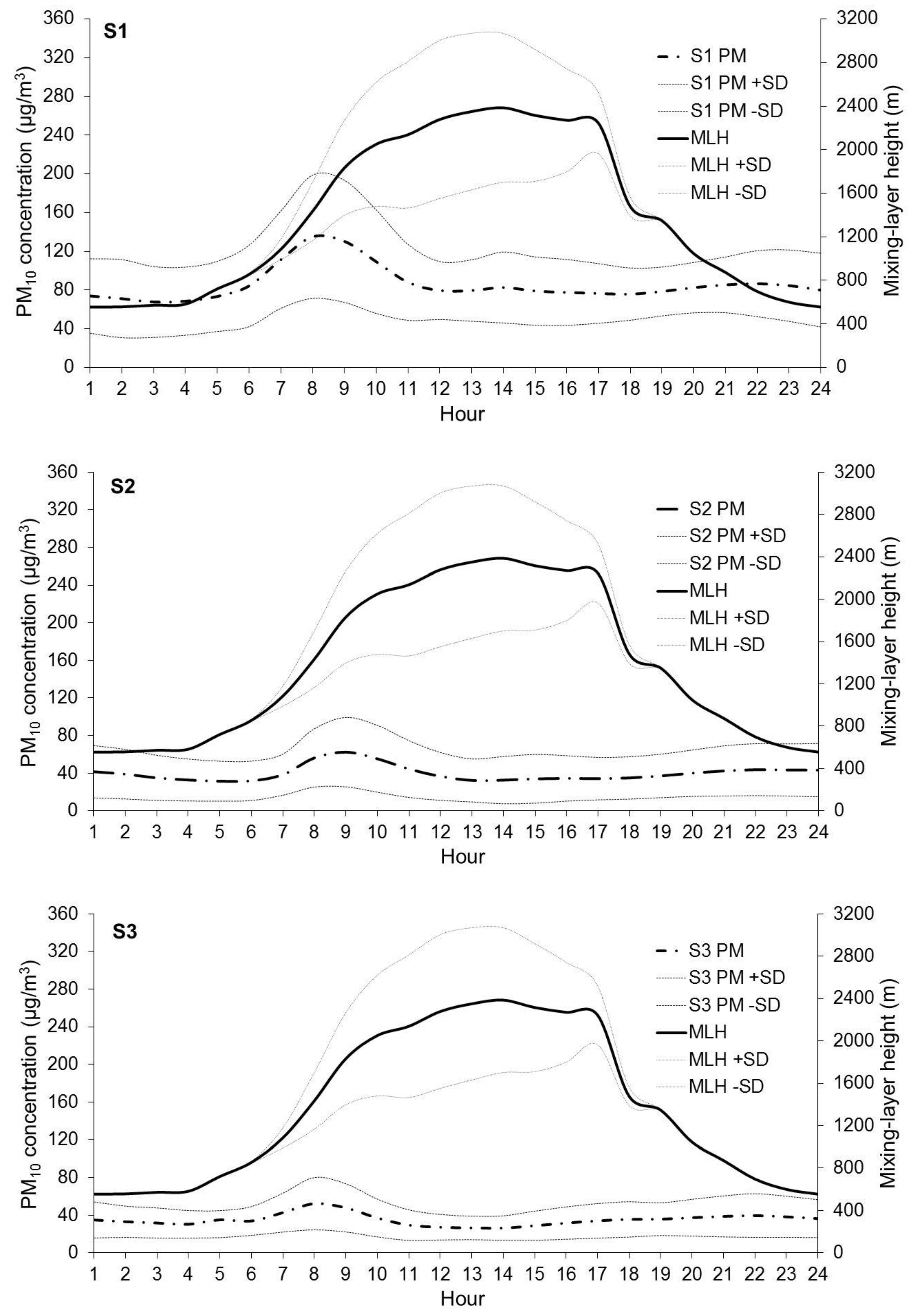
For all stations, an increase in the average PM10 concentration was detected at 5 a.m. and a decrease was detected between 11 a.m.–12:00 p.m. Peaks in PM10 concentrations were detected between 8–9 a.m. These maximum events in hourly PM10 concentrations coincided with the maximum traffic intensities, which preceded the start of standard work activities in Bogota. These hourly episodes of increase in PM10 concentration were also preceded by low heights of mixing-layer, between 722 m (SD = 5.0) and 1085 m (SD = 95.0 m). The results revealed a similar trend in hourly PM10 concentrations for all stations throughout the research period (Figure 2). A Spearman’s correlation analysis for all stations displayed medium positive relationships (rs-Spearman between 0.410–0.506; Table 2). The results also showed a similar trend for DPM10 in this research. A Spearman’s correlation analysis for all stations displayed positive relationships with a tendency for medium values (rs-Spearman between 0.355–0.507). On average, S1 showed the highest DPM10. Daily concentrations in S1 were 115% and 146% higher than those observed in S2 and S3, respectively.
3.2. Air Quality Standards
The results indicated that S1 station exceeded the daily Colombian limit 31% of the time (PE) during the research period, but especially during February, where the average daily PM10 concentration was 107.8 μg/m3 (Figure 3). During that month, the daily limit was exceeded 54.1% of the time. In contrast, DPM10 of the stations S2 and S3 complied with the Colombian limit 99.5% and 100% of the time during the research period, respectively. It was found that the monthly average of PM10 concentrations in the S1 and S2 stations represented a public health risk during all months (PM10 > 71 µg/m3; DM > 1.49%; PE = 96.6%) and in February (PM10 = 52.2 µg/m3; DM = 0.156%; PE = 48.8%), respectively, according to the daily limit established by WHO. The S3 station showed the lowest public health risk, exceeding the daily limit 13.0% of the time during the research period.
The order of precedence established by quartiles (Q) to evaluate the risk per daily exposure to PM10 showed on average that the first three months of the year were Q1 in all stations (S1: PM10 = 101.1 µg/m3, PE = 99.2%; S2: PM10 = 48.2 µg/m3, PE = 44.0%; S3: PM10 = 42.4 µg/m3, PE = 24.4%). February was highlighted as the highest risk for public health, followed in order of precedence for March and January. In contrast, Q4 months or lowest risk for public health were in order of precedence July, June, and August (S1: PM10 = 80.9 µg/m3, PE = 93.9%; S2: PM10 = 32.7 µg/m3, PE = 12.9%; S3: PM10 = 27.4 µg/m3, PE = 2.84%). During the Q4 months an increase in daytime MLH was also observed (Figure 3).
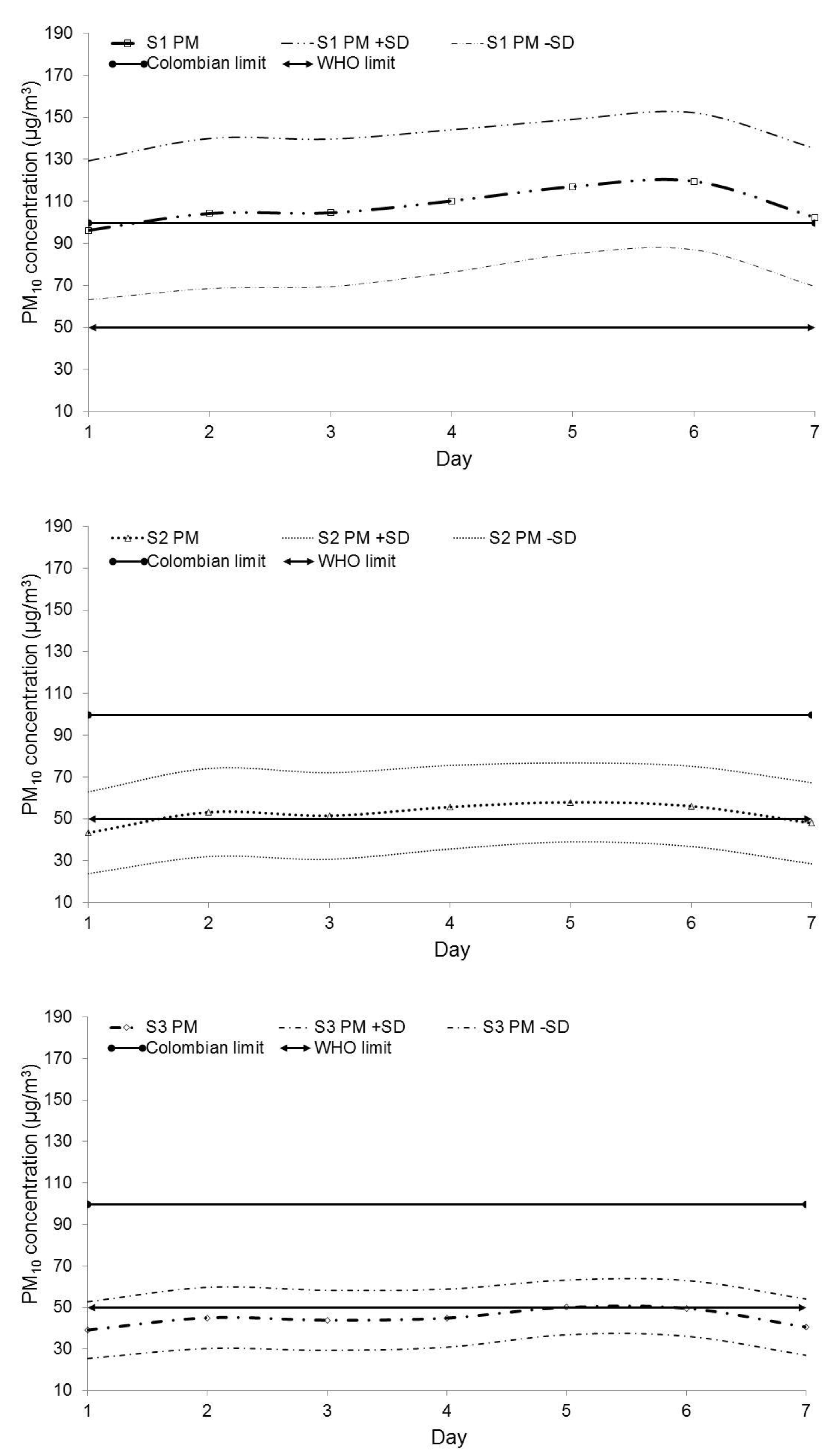
During the month of greatest public health risk (February), the variations of PM10 concentration during the days of the week in relation to the referenced limits (24-h exposure time) were studied. On average, the results revealed that at S1 station the PM10 concentrations represented a public health risk during most days of the week in relation to Colombian limit, except for the exposure period between Sunday and Monday (PM10 = 96.2 µg/m3). The previous trend was similar in the S1 and S2 stations from the daily limit established by WHO (Figure 4). The S3 station was the only one that complied during February to the referenced limits in this research; except during the exposure period between Friday and Saturday (PM10 = 50.1 µg/m3).
A monthly analysis with Spearman’s coefficient showed, on average and for all stations, a very strong positive relationship between DPM10 and PE relative to the daily WHO limit (rs-Spearman = 0.974, p-value < 0.001). A linear regression model between DPM10 (µg/m3) and PE (%) was developed (PE = 1.30 × DPM10 − 27.4; R2 = 0.938). A monthly analysis with the Spearman’s coefficient also showed on average for all stations a very strong positive relationship between PE and DM relative to the WHO limit (rs-Spearman = 0.873, p-value < 0.001). A linear regression model between PE (%) and DM (%) was developed (DM = 0.0313 × PE + 0.146; R2 = 0.848).
3.3. AC
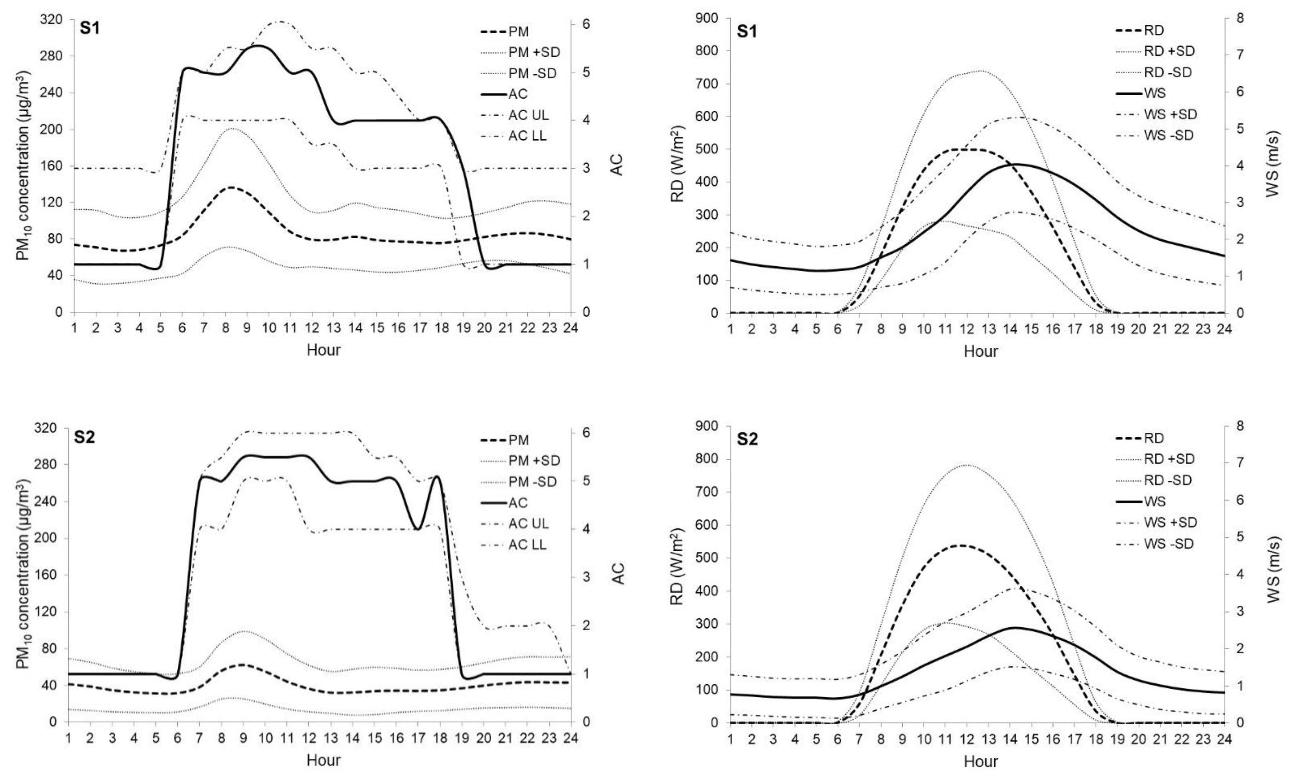
Figure 5 displays the average hourly AC from the quantitative scale considered in this research. This figure also displays the variation range of AC (lower limit and upper limit). On average, dominant AC between 6–18 h (daytime) was slightly unstable (AC = 4, frequency for 24 h, f-24 h = 19.5%; variation range: 3–6), unstable (AC = 5, f-24 h = 22.7%; variation range: 4–6), and unstable (AC = 5, f-24 h = 24.5%; variation range: 4–6) for stations S1, S2, and S3, respectively. During the daytime RD and WS were as follows: S1 (RD = 288 W/m2, SD = 135; WS = 2.77 m/s, SD = 1.09), S2 (RD = 304 W/m2, SD = 145; WS = 1.75 m/s, SD = 0.83), and S3 (RD = 352 W/m2, SD = 163; WS = 1.46 m/s, SD = 0.69). As for the dominant AC between 19–5 h (nighttime) was stable (AC = 1, f-24 h) for stations S1, S2, and S3: 22.9% (variation range: 1–3), 39.5% (variation range: 1–3), and 45.8% (variation range: 1–2), respectively. On average, during this period RD and WS were lower relative to the daytime: S1 (RD = 0.02 W/m2, SD = 0.23; WS = 1.64 m/s, SD = 0.80), S2 (RD = 0.57 W/m2, SD = 2.33; WS = 0.87 m/s, SD = 0.58), and S3 (RD = 0.31 W/m2, SD = 3.23; WS = 0.61 m/s, SD = 0.39).
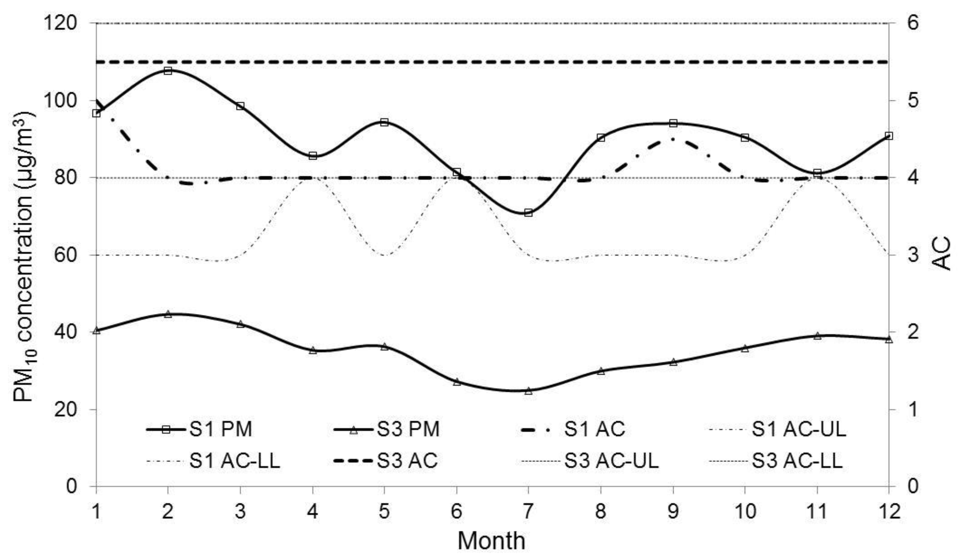
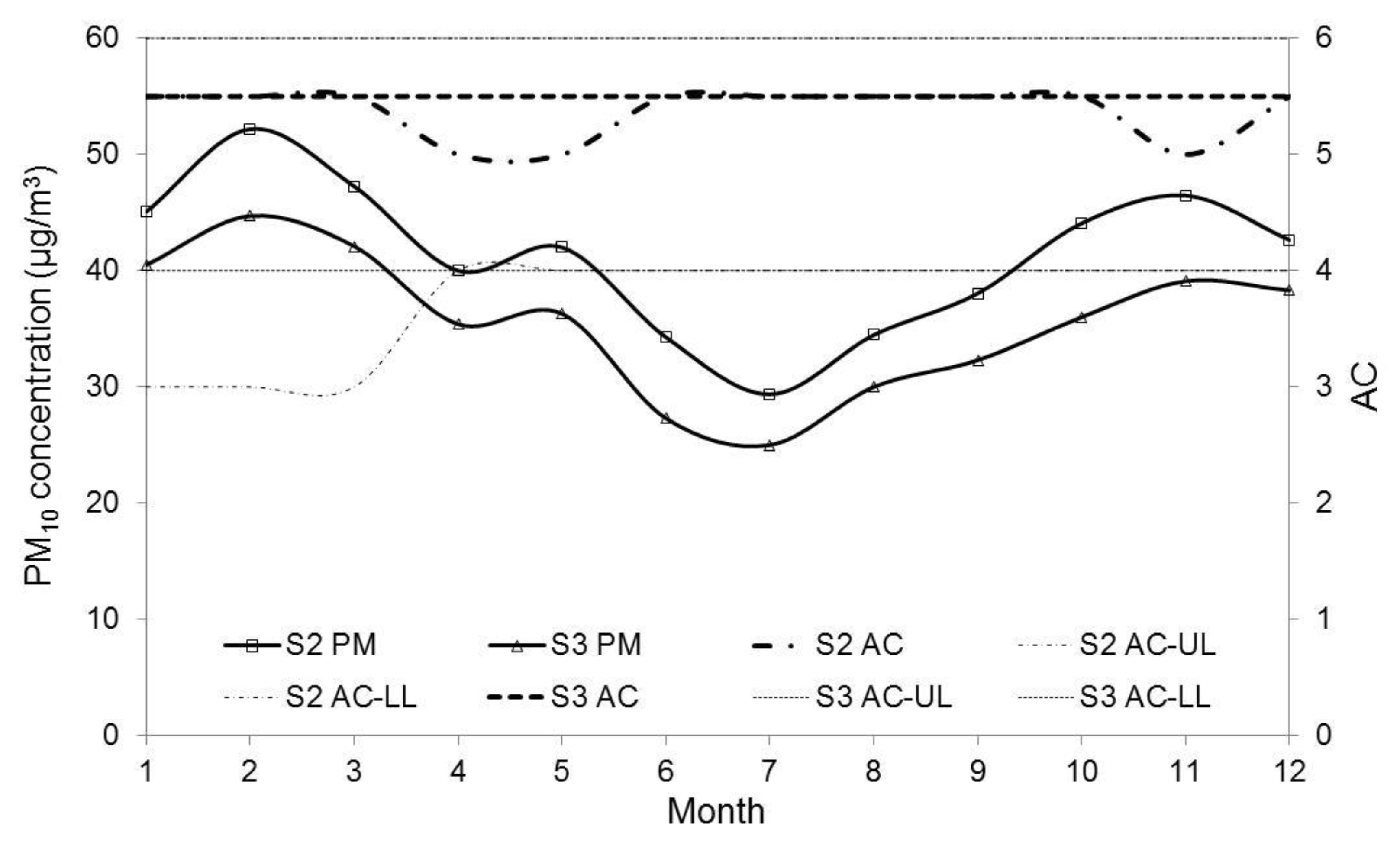
On average, for the whole research area, the results indicated that the dominant hourly AC during the daytime was slightly unstable and unstable (AC between 4 and 5.5; f-24 h = 46.1%). At nighttime, the dominant hourly AC was stable (AC = 1; f-24 h = 36.1%). A Kruskal-Wallis test between the stations S1, S2, and S3 revealed that there were no significant hourly variations in average AC (p-value = 0.827). Namely, there was probably a similar trend in hourly AC during the research period for all stations. However, the monthly, by comparison, showed, on average, that the order of precedence for daytime AC was as follows: S3 (AC = 5.5, variation range: 4–6) > S2 (AC = 5.38, variation range: 3–6) > S1 (AC = 4.13, variation range: 3–6). Indeed, the order of precedence for RD was similar: S3 (RD = 352 W/m2, SD = 163) > S2 (RD = 304 W/m2, SD = 145) > S1 (RD = 288 W/m2, SD = 135). The results also showed an order of precedence opposite for PM10 concentrations: S1 (90.2 µg/m3) > S2 (41.3 µg/m3) > S3 (35.6 µg/m3) (Figure 6).
An hourly analysis with Spearman’s coefficient showed on average for all stations a positive relationship of considerable to very strong between MLH and RD (rs-Spearman = 0.911, p-value < 0.001), and MLH and WS (rs-Spearman = 0.859, p-value < 0.001). Linear regression models were developed between MLH and RD (MLH = 2.92 × RD + 870; R2 = 0.778), and MLH and WS (MLH = 870 × WS + 7.79; R2 = 0.835). Finally, a linear regression model was developed integrating RD and WS (MLH = 2.91 × [RD + WS] + 866; R2 = 0.780).
3.4. LC
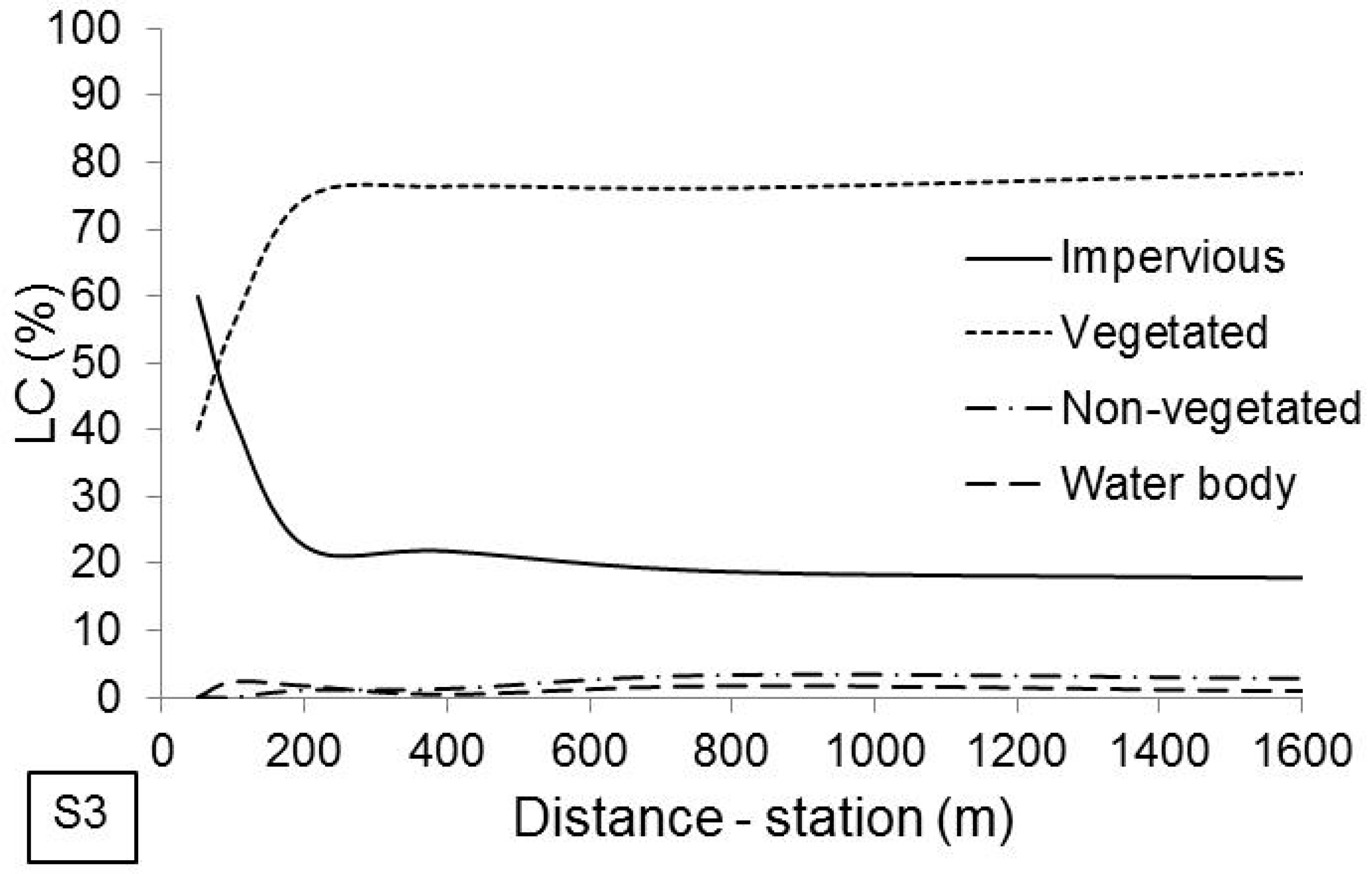
Figure 7 displays the variation in the LC type for the influence distances for each station. One station exhibited mainly impervious LC (S1). This type of LC represented between 54.5–85.8% of the zone covered by that station, when using the influence distance considered for each station (between 50–1600 m). The precedence order for this LC in the stations was S1 > S2 > S3. Otherwise, one station exhibited mainly vegetated LC (S3). This type of LC represented between 40.1–78.4% of the zone covered by that station. The precedence order for this LC in the stations was S3 > S2 > S1. As noted, in this research, there was one station with mainly impervious LC (S1) and one with mainly vegetated LC (S3). The S2 station had intermediate values of vegetated and impervious LC.
3.5. PM10 Information Analysis
Table 3 displays the terms AR/I/MA, model constant, transformation type, R2, root-mean-square error, mean-absolute percentage error, Ljung-Box Q’ statistic (p-value), and normalized Bayesian information criterion of the models generated for DPM10. ARIMA models with a p-value (Q’) > 0.05 were considered satisfactory [47]. The results revealed an ARIMA model of higher order in the AR term for the station with impervious LC prevalence (S1, AR = 2) compared to the station with vegetated LC prevalence (S3, AR = 1). ARIMA models generated for the station with vegetated LC prevalence showed higher orders in the MA term (S3, between 2–3) compared to the station with impervious LC prevalence (S1, MA = 2). Finally, Table 4 displays the parameter estimates for the model terms selected for DPM10.
4. Discussion
4.1. Public Health Considerations
On an hourly basis, the results suggest a similar trend in PM10 concentrations between all stations (rs-Spearman between 0.483–0.506; see Table 2). This trend was probably related to the uniform trend in the PM10 emission cycles by mobile (vehicles), fixed (industries), and natural sources in the research areas. The stations selected in this research covered 21.9 km with relation to the 33 km length of the city from north to south (Figure 1). Thus, the results display that this uniform trend in the hourly PM10 emission cycles was probably similar in all sectors of Bogota. All stations considered in this research were of background type. The previous trend could also have been due to the high PM10 levels observed throughout the city (average DPM10 of up to 107.8 µg/m3).
On an hourly timescale, the results allowed us to detect the most critical time interval for PM10. On average, this time interval was from 6–11 a.m., with maximum PM10 concentrations between 8–9 a.m. (PM10−S1 = 135 µg/m3, SD = 63.1; PM10−S2 = 62.4 µg/m3, SD = 36.9; PM10−S3 = 52.3 µg/m3, SD = 25.6; see Figure 2). The reference legislation made it possible to demonstrate that the most critical station within the public health framework was S1 (Figure 3). On average, this station exceeded the daily Colombian limit during February by 7.8%, and the daily WHO limit for all months by 80.4%. DPM10 observed in February at S1 (107.8 µg/m3) could increase the DM by 4.10% (PE = 100%) with relation to the DM observed for a concentration of 50 µg/m3 [41]. According to WHO (2005), an increase in DM of 5.0% requires immediate corrective measures. On average for all months, around the S1 station there was probably an increase of 2.85% in DM during the research period (PE = 96.6%). This station was located to the Southwest of Bogota (Figure 1). Some researchers also reported that an increase of 50 μg/m3 in urban DPM10 generated an increase of 2.10% in DM [6]. The stations S2 and S3 did not exceed the daily Colombian limit during all months, and S2 station was the only one that exceeded the daily WHO limit (in February, PE = 48.8%). After this study, Colombian legislation decreased the 24-h limit to 75 µg/m3 [48].
On average, during Q1 months the DPM10 were 11.5%, 16.8%, and 35.9% higher than those observed in the Q2, Q3, and Q4 months, respectively (Figure 3). Indeed, during Q1 months the PE increased by 23.2%, 22.3%, and 53.2%, respectively. During the Q4 months an increase in daytime MLH was also observed (between 1625–1828 m, SD: 276–279), probably influenced by high RD (239–294 W/m2, SD: 148–179) and high WS (1.87–2.91 m/s, SD: 1.20–1.78) during these months. The results suggested that public health surveillance and control agencies should plan and implement different strategies according to the monthly Q value. On average, DM during Q1 months could be increased by between 1.07–1.43% in relation to DM of Q4 months.
From the linear regression models developed, very strong positive relationships were suggested between DPM10 and PE (rs-Spearman = 0.974), and between PE and DM (rs-Spearman = 0.873). On a monthly basis, the results suggested on average a 13.0% increase in PE for each 10 µg/m3 increase in DPM10. The findings also suggested a 0.313% increase in DM for each 10% increase in PE. Thus, the above findings could be useful to comprehensively assess the effectiveness of air pollution control measures in relation to PM10. Namely, the effects on PE and DM could also be directly assessed with the regression models developed in this research.
On average, the results showed an increase in DPM10 as the week progressed, reaching its maximum level during the exposure period between Thursday–Saturday (Figure 4). PM10 concentrations during this exposure period exceeded the daily Colombian limit in S1 station (15.6%), and daily WHO limit in the S1 and S2 stations (S1 = 131%; S2 = 12.9%). S3 station complied with all legislative limits of reference, except during the exposure period between Friday–Saturday. A similar trend in DPM10 for other months was observed. Therefore, the results suggested this exposure period (Thursday–Saturday) as the highest risk during the week with relation to the possible PM10 impact on human health. The results also suggested that restrictions on industrial activities and motor vehicle circulation, as well as wet road cleaning, should be more stringent during this exposure period.
On a weekly basis, during the whole research period, the highest DPM10 tended to occur during the exposure period between Friday–Saturday. On average, concentrations during this exposure period were higher (S1 = 14.3%, S2 = 13.3%, and S3 = 16.8%) compared to the concentrations observed during the exposure period between Sunday–Friday. This trend was probably because in Bogota there was a restriction on vehicular movement due to traffic congestion between Monday–Friday. This traffic restriction prevented the use of 40% of the city’s vehicles between 6–9 a.m. and 3–7 p.m. (between 425,000–817,000 motor vehicles). Namely, there was no traffic restriction on Saturdays, which probably explained the increase in DPM10 for this day at all stations (average increase of 14.8%). The results also showed a higher increase in DPM10 on S3 station for this day in relation to the other stations under study (between 2.50–3.50%). This trend could be due to the land use existing in S3 station, which was associated with lower PM10 concentrations. Unlike the other stations under study, the land around this station did not have an industrial and commercial use (Table 1), but rather, was residential and institutional (schools and universities). On the other hand, the large values of PM10 concentrations at S1 on Saturdays could also be explained by greater sediment resuspension as traffic increases. This station has the largest area of impervious LC and greatest road sediment loadings [49].
4.2. AC and LC
With relation to the influence of AC, the results probably showed the best possible scenario from a public health viewpoint for maximum hourly PM10 concentrations. Namely, the maximum concentrations recorded by the stations S1 (135 µg/m3, SD = 63.1), S2 (62.4 µg/m3, SD = 36.9), and S3 (52.3 µg/m3, SD = 25.6) occurred during daytime periods (8–9 a.m.), when on average the dominant AC was between unstable and very unstable (Figure 5). This suggested high PM10 dispersion and, therefore, a probable reduction in hourly concentration during these extreme pollution episodes. Otherwise, the maximum hourly PM10 concentrations in Bogota during daytime probably would have been higher. Though, these extreme pollution episodes were probably preceded by low MLH, on average between 722–1085 m (SD: 5.0–95.0). Indeed, low RD (0.28–54.2 W/m2, SD: 1.99–31.9) and low WS (0.77–0.85 m/s, SD: 0.50–0.52) were also observed during these periods (Figure 5; 5–7 a.m.). On average, we also observed a rapid change in AC (from stable to unstable) over a short period of time at sunrise (5–7 a.m.) probably due to a significant increase in RD (+53.8 W/m2).
The results revealed that during nighttime, the dominant AC was stable (AC = 1). This suggested low PM10 dispersion during these time periods, and therefore, a probable increase in hourly concentrations. The best possible scenario in the public health framework for S1 and S2 stations occurred during nighttime periods when the lowest hourly PM10 concentrations were observed (Figure 5). On average, nighttime PM10 concentrations in S1 and S2 stations were 20.9% and 4.61% lower than those observed during the daytime, respectively. Though, hourly PM10 concentrations at S3 were different. On average, at this station the nighttime PM10 concentrations were 1.39% higher than those observed during the daytime, despite a probable decrease in the emission sources of PM10 such as traffic. This trend could probably be due to the land use existing in S3 station, which associated the lowest PM10 concentrations (average DPM10 = 34.9 µg/m3) in relation to the other stations (S1 = 85.9 µg/m3; S2 = 40.0 µg/m3). Unlike the other stations under study, the land around the S3 station did not have an industrial and commercial use (Table 1), but rather, was residential and institutional (schools and universities). The results also suggested that the increase in nighttime PM10 concentrations at S3 was probably associated with the dominant AC, which were stable. Some researchers informed a similar trend under dominant conditions of nighttime AS (AC = 1) in the cities of Seoul (Korea) and Milan (Italy), respectively; despite a reduction in the PM10 emission sources (traffic and industries) [19,20].
The results indicated that at the S3 station, there was a lower difference (1.39%) between daytime and nighttime concentrations of hourly PM10 in relation to the stations S1 (20.9%) and S2 (4.61%). This trend was also supported by a lower hourly variation in PM10 concentrations in S3 station (S3, SD = 6.27 µg/m3; S2, SD = 8.18 µg/m3; S1, SD = 17.8 µg/m3). As mentioned, S3 station had comparatively the highest degree of AI during daytime (S3, AC = 5.5, variation range: 4–6; S2, AC = 5.38, variation range: 3–6; S1, AC = 4.13, variation range: 3–6) and during nighttime there were no differences among stations in hourly AC (AC = 1; see Figure 5). Thus, the results suggested that the stations located in urban sectors with greater AI probably tended to show lower concentrations and variations of hourly PM10.
From the linear regression models developed, we observed positive relationships from considerable to very strong between MLH and RD (rs-Spearman = 0.911), and MLH and WS (rs-Spearman = 0.859). In this study, the results suggested comparatively that there was a greater association between MLH and RD in comparison with WS. On average, we observed an increase of 292 m in MLH for each increase of 100 W/m2 in RD. We also observed an increase of 870 m in MLH for each increase of 1.0 m/s in WS. Indeed, the results suggested a positive relationship between MLH and the degree of AI. The monthly results revealed, on average, that the DPM10 were lower in the station associated with the highest degree of AI (S3). The order of precedence in the degree of AI for stations was as follows: S3 > S2 > S1 (Figure 6). The order of precedence for DPM10 was as follows: S1 > S2 > S3. The results in this research suggested an inverse relationship between DPM10 and AI.
Additionally, a probable relationship was detected between AI and LC type. The results showed that urban sectors of greater AI were characterized by a mainly vegetated LC (S3 = 78.4%; Figure 7). In contrast, urban sectors of lower AI were related with mainly impervious LC (S1 = 85.8%). The previous analysis was conducted within a 1600-m radius in relation to the physical location of the stations, because it has been reported that this was probably the best distance to observe differences between DPM10 and LC [17]. Studies in urban sectors have also reported an important influence of a vegetated LC on DPM10. For example, some researchers informed that the existence of trees in Wuhan (China) decreased the DPM10 between 7–15% [14]. A vegetated LC also acted as an effective remover for particulate and gaseous atmospheric pollutants [22]. On average, in this research the sectors with mainly vegetated LC (S3) showed a DPM10 lower (59.4%) compared to the sectors of mainly impervious LC (S1).
A correlation analysis among the influence distances (50–1600 m) and LC types around each station revealed that the S2 station exhibited the best correlations (rs-Spearman, significant correlations = 47.2%; p-values < 0.05). This analysis also allowed us to identify that the distance with the worst correlations was 1600 m (rs-Spearman, significant correlations = 33.3%, p-values < 0.05). Namely, this influence distance was the one that generated the least association between all stations considered in this research (Figure 7). Thus, in this research, we chose S2 as the station to compare the ARIMA models generated; and we also select at 1600 m as the influence distance to study the likely differences among models.
The findings revealed a difference between stations for the impervious LC distribution: 85.8% at S1, 56.5% at S2, and 17.9% at S3. Outcomes for the AR term of the models imply that these differences were related to the LC type. To increase the impervious LC around a station, an increase in the AR term was assumed (Table 3). More impervious LC around a station meant that the DPM10 of preceding days had a stronger influence. In this research, the PM10 concentrations persistence was around two days (S1 and S2 stations, AR = 2). A greater PM10 pollution persistence was detected in urban sectors with more impervious LC (roofs/pavements/footpaths) and less vegetated LC (trees/grasslands). Some researchers also applied models of order 1 and 2 in the AR term simulated DPM10 in the high-pollution cities of New Delhi (India) and Temuco (Chile), respectively [43,44].
The MA term of the models showed a difference that was probably related to vegetated LC (10.9% at S1, 39.3% at S2, and 78.4% at S3). The findings indicated that stations with more vegetated LC (S2 and S3) showed a higher order in the MA term (Table 3). More vegetated LC around a station meant a greater effect exerted by the PM10 variations of preceding days. In this research, the effect was observed 2–3 days prior to measurement (MA between 2–3). Consequently, the results also pointed to mainly vegetated LC sectors as those displaying greater variability in DPM10. These results infer that in sectors with mainly impervious LC, particulate matter sources probably had a more uniform tendency in the daily emission cycles, as shown by lower variability in DPM10 (S1 station, MA = 2) compared to sectors with more vegetated LC (S2 and S3 stations, MA between 2–3).
5. Conclusions
The results suggest a similar temporal trend for PM10 throughout the megacity of Bogota, probably due to the high concentrations observed at the stations (DPM10 of up to 107.8 µg/m3). On average, the findings also imply that within the city limit, different atmospheric conditions may coexist. In effect, urban sectors with lower AI show higher DPM10 (between 131–144%) compared to urban sectors of greater AI, with the former showing an increase in DM of 2.85% compared to the latter. Thus, urban LC type can probably be used as a public health indicator, because in urban sectors where impervious LC predominates (85.8%) over vegetated LC (78.4%), greater increases in DM (+2.85%) and PE (+84.6%) were observed. An ARIMA analysis also showed that a more impervious LC around a station greater influences the PM10 concentrations of the previous days. The persistence of PM10 concentrations is probably two days, i.e., extreme PM10 episodes possibly persist for two days in Bogota. Extreme pollution episodes are probably also preceded by low MLH (between 722–1085 m).
Additionally, in this high-altitude megacity, DM during Q1 months (highest risk) increased between 1.07–1.43% in relation to DM of Q4 months (lowest risk). Indeed, the findings showed, on average, a 13.0% increase in PE for each 10 µg/m3 increase in DPM10, and a 0.313% increase in DM for each 10% increase in PE. The average reduction of 14.8% in DPM10 (−0.79% in DM) was probably due to 40% restriction of the traffic at peak hours (6–9 a.m. and 3–7 p.m.). On average, this traffic restriction is probably more effective in urban sectors with vegetated LC (up to −3.50% in DPM10) in comparison to urban sectors with impervious LC. This predominant land use in vegetated LC (residential/institutional) also probably leads to higher nighttime PM10 concentrations (1.39%) in relation to the daytime concentrations, despite a decrease in traffic and industrial and commercial activity. Lastly, the outcomes of this research serve to extend our knowledge about the behavior of DPM10 concentrations and the influences of AC and LC, allowing us to develop and implement different strategies for the surveillance and control of such metrics for public health in high-pollution megacities.
Author Contributions
Conceptualization, C.Z., J.S. and J.E.P.; Data curation, C.Z. and J.S.; Formal analysis, C.Z. and J.S.; Funding acquisition, C.Z.; Investigation, C.Z. and J.S.; Methodology, C.Z., J.S. and J.E.P.; Project administration, C.Z.; Resources, C.Z. and J.S.; Software, C.Z.; Supervision, C.Z.; Validation, C.Z., J.S. and J.E.P.; Visualization, C.Z. and J.S.; Writing-original draft, C.Z.; Writing-review & editing, J.S. and J.E.P. All authors have read and agreed to the published version of the manuscript.
Funding
This research received no external funding.
Institutional Review Board Statement
Not applicable.
Informed Consent Statement
Not applicable.
Data Availability Statement
Restrictions apply to the availability of these data. Data was obtained from Red de Monitoreo de Calidad del Aire de Bogotá (RMCAB) and are available at http://201.245.192.252:81/Report/stationreport with the permission of RMCAB.
Acknowledgments
The authors wish to thank the Universidad Distrital Francisco José de Caldas and Bogota Environment Secretariat (Colombia).
Conflicts of Interest
The author states that there is no conflict of interest.
Nomenclature
| AC | Atmospheric condition. |
| AI | Atmospheric instability. |
| ARIMA | Autoregressive integrated moving average. |
| AS | Atmospheric stability. |
| BIC | Normalized Bayesian information criterion. |
| DM | Daily mortality. |
| DPM10 | Daily PM10 concentrations. |
| LC | Land coverage. |
| MAPE | Mean-absolute percentage error. |
| MLH | Mixing-layer height. |
| N.C. | Model without constant. |
| PE | Excess percentage. |
| PM | Particulate material. |
| RD | Solar radiation. |
| RMSE | Root-mean-square error. |
| SD | Standard deviation. |
| WHO | World Health Organization. |
| WS | Wind speed. |
References
- Dahari, N.; Latif, M.T.; Muda, K.; Hussein, N. Influence of Meteorological Variables on Suburban Atmospheric PM2.5 in the Southern Region of Peninsular Malaysia. Aerosol Air Qual. Res. 2020, 20, 14–25. [Google Scholar] [CrossRef]
- Ning, X.; Ji, X.; Li, G.; Sang, N. Ambient PM2.5 causes lung injuries and coupled energy metabolic disorder. Ecotoxicol. Environ. Saf. 2019, 170, 620–626. [Google Scholar] [CrossRef] [PubMed]
- Maesano, C.N.; Morel, G.; Matynia, A.; Ratsombath, N.; Bonnety, J.; Legros, G.; Da Costa, P.; Prud’homme, J.; Annesi-Maesano, I. Impacts on human mortality due to reductions in PM10 concentrations through different traffic scenarios in Paris, France. Sci. Total Environ. 2020, 698, 134257. [Google Scholar] [CrossRef]
- Zhu, X.; Qiu, H.; Wang, L.; Duan, Z.; Yu, H.; Deng, R.; Zhang, Y.; Zhou, L. Risks of hospital admissions from a spectrum of causes associated with particulate matter pollution. Sci. Total Environ. 2019, 656, 90–100. [Google Scholar] [CrossRef]
- Dockery, D.W.; Pope, C.A.; Xu, X.; Spengler, J.D.; Ware, J.H.; Fay, M.E.; Ferris, B.G.; Speizer, F.E. An Association between Air Pollution and Mortality in Six U.S. Cities. N. Engl. J. Med. 1993, 329, 1753–1759. [Google Scholar] [CrossRef] [PubMed] [Green Version]
- Katsouyanni, K.; Schwartz, J.; Spix, C.; Touloumi, G.; Zmirou, D.; Zanobetti, A.; Wojtyniak, B.; Vonk, J.M.; Tobias, A.; Pönkä, A.; et al. Short term effects of air pollution on health: A European approach using epidemiologic time series data: The APHEA protocol. J. Epidemiol. Community Health 1996, 50, S12–S18. [Google Scholar] [CrossRef] [Green Version]
- Liu, W.; Xu, Z.; Yang, T. Health Effects of Air Pollution in China. Int. J. Environ. Res. Public Health 2018, 15. [Google Scholar] [CrossRef] [PubMed] [Green Version]
- Rodríguez-Villamizar, L.A.; Rojas-Roa, N.Y.; Fernández-Niño, J.A. Short-term joint effects of ambient air pollutants on emergency department visits for respiratory and circulatory diseases in Colombia, 2011–2014. Environ. Pollut. 2019, 248, 380–387. [Google Scholar] [CrossRef] [PubMed]
- Blanco-Becerra, L.C.; Miranda-Soberanis, V.; Hernández-Cadena, L.; Barraza-Villarreal, A.; Junger, W.; Hurtado-Díaz, M.; Romieu, I. Effect of particulate matter less than 10 µm (PM10) on mortality in Bogota, Colombia: A time-series analysis, 1998–2006. Salud Publica Mex. 2014, 56, 363–370. [Google Scholar] [CrossRef] [Green Version]
- Breuer, J.L.; Samsun, R.C.; Peters, R.; Stolten, D. The impact of diesel vehicles on NOx and PM10 emissions from road transport in urban morphological zones: A case study in North Rhine-Westphalia, Germany. Sci. Total Environ. 2020, 727, 138583. [Google Scholar] [CrossRef] [PubMed]
- Achad, M.; López, M.L.; Ceppi, S.; Palancar, G.G.; Tirao, G.; Toselli, B.M. Assessment of fine and sub-micrometer aerosols at an urban environment of Argentina. Atmos. Environ. 2014, 92, 522–532. [Google Scholar] [CrossRef]
- Palacio-Soto, D.F.; Zafra-Mejía, C.A.; Rodríguez-Miranda, J.P. Evaluation of the air quality by using a mobile laboratory: Puente Aranda (Bogotá D.C.; Colombia). Rev. Fac. Ing. Univ. Antioquia 2014, 2, 153–166. [Google Scholar]
- Seinfeld, J.H.; Pandis, S.N. Atmospheric Chemistry and Physics: From Air Pollution to Climate Change; John Wiley & Sons: Hoboken, NJ, USA, 2016. [Google Scholar]
- Chen, X.; Pei, T.; Zhou, Z.; Teng, M.; He, L.; Luo, M.; Liu, X. Efficiency differences of roadside greenbelts with three configurations in removing coarse particles (PM10): A street scale investigation in Wuhan, China. Urban For. Urban Green. 2015, 14, 354–360. [Google Scholar] [CrossRef]
- Fortelli, A.; Scafetta, N.; Mazzarella, A. Influence of synoptic and local atmospheric patterns on PM10 air pollution levels: A model application to Naples (Italy). Atmos. Environ. 2016, 143, 218–228. [Google Scholar] [CrossRef] [Green Version]
- Srinivas, C.V.; Venkatesan, R.; Somayaji, K.M.; Indira, R. A simulation study of short-range atmospheric dispersion for hypothetical air-borne effluent releases using different turbulent diffusion methods. Air Qual. Atmos. Health 2009, 2, 21–28. [Google Scholar] [CrossRef] [Green Version]
- Zafra, C.; Ángel, Y.; Torres, E. ARIMA analysis of the effect of land surface coverage on PM10 concentrations in a high-altitude megacity. Atmos. Pollut. Res. 2017, 8, 660–668. [Google Scholar] [CrossRef]
- Chambers, S.D.; Wang, F.; Williams, A.G.; Xiaodong, D.; Zhang, H.; Lonati, G.; Crawford, J.; Griffiths, A.D.; Ianniello, A.; Allegrini, I. Quantifying the influences of atmospheric stability on air pollution in Lanzhou, China, using a radon-based stability monitor. Atmos. Environ. 2015, 107, 233–243. [Google Scholar] [CrossRef]
- Lee, S.; Ho, C.H.; Lee, Y.G.; Choi, H.J.; Song, C.K. Influence of transboundary air pollutants from China on the high-PM10 episode in Seoul, Korea for the period October 16–20, 2008. Atmos. Environ. 2013, 77, 430–439. [Google Scholar] [CrossRef]
- Vecchi, R.; Marcazzan, G.; Valli, G. A study on nighttime–daytime PM10 concentration and elemental composition in relation to atmospheric dispersion in the urban area of Milan (Italy). Atmos. Environ. 2007, 41, 2136–2144. [Google Scholar] [CrossRef]
- Shan, Y.; Jingping, C.; Liping, C.; Zhemin, S.; Xiaodong, Z.; Dan, W.; Wenhua, W. Effects of vegetation status in urban green spaces on particle removal in a street canyon atmosphere. Acta Ecol. Sin. 2007, 27, 4590–4595. [Google Scholar] [CrossRef]
- Han, D.; Shen, H.; Duan, W.; Chen, L. A review on particulate matter removal capacity by urban forests at different scales. Urban For. Urban Green. 2020, 48, 126565. [Google Scholar] [CrossRef]
- Irga, P.J.; Burchett, M.D.; Torpy, F.R. Does urban forestry have a quantitative effect on ambient air quality in an urban environment? Atmos. Environ. 2015, 120, 173–181. [Google Scholar] [CrossRef] [Green Version]
- Minguillón, M.C.; Querol, X.; Baltensperger, U.; Prévôt, A.S.H. Fine and coarse PM composition and sources in rural and urban sites in Switzerland: Local or regional pollution? Sci. Total Environ. 2012, 427–428, 191–202. [Google Scholar] [CrossRef] [PubMed]
- Wolf-Benning, U.; Draheim, T.; Endlicher, W. Spatial and temporal differences of Particulate Matter in Berlin. Int. J. Environ. Waste Manag. 2009, 4, 3–16. [Google Scholar] [CrossRef]
- Titos, G.; Lyamani, H.; Pandolfi, M.; Alastuey, A.; Alados-Arboledas, L. Identification of fine (PM1) and coarse (PM10-1) sources of particulate matter in an urban environment. Atmos. Environ. 2014, 89, 593–602. [Google Scholar] [CrossRef] [Green Version]
- Waked, A.; Favez, O.; Alleman, L.Y.; Piot, C.; Petit, J.E.; Delaunay, T.; Verlinden, E.; Golly, B.; Besombes, J.L.; Jaffrezo, J.L.; et al. Source apportionment of PM10 in a north-western Europe regional urban background site (Lens, France) using positive matrix factorization and including primary biogenic emissions. Atmos. Chem. Phys. 2014, 14, 3325–3346. [Google Scholar] [CrossRef] [Green Version]
- Liu, J.; Mo, L.; Zhu, L.; Yang, Y.; Liu, J.; Qiu, D.; Zhang, Z.; Liu, J. Removal efficiency of particulate matters at different underlying surfaces in Beijing. Environ. Sci. Pollut. Res. 2016, 23, 408–417. [Google Scholar] [CrossRef]
- De Montoya, G.J.; Cepeda, W.; Eslava, J.A. Características de la turbulencia y de la estabilidad atmosférica en Bogotá. Rev. Acad. Colomb. Cienc. Exactas Físicas Nat. 2004, 28, 327–335. [Google Scholar]
- Sarmiento, R.; Hernández, L.J.; Medina, E.K.; Rodríguez, N.; Reyes, J. Respiratory symptoms associated with air pollution in five localities of Bogotá, 2008-2011, a dynamic cohort study. Biomédica 2015, 35, 167–176. [Google Scholar] [CrossRef] [Green Version]
- SDA. Documento Técnico de Soporte, Modificación del Decreto 98 de 2011 [WWW Document]. 2017. Available online: http://www.ambientebogota.gov.co/c/document_library/get_file?uuid=d134928c-8756-4a69-ad18-ff09bb822fef&groupId=3564131 (accessed on 9 January 2021).
- U.S.EPA. Compendium of Methods for the Determination of Inorganic Compounds in Ambient Air [WWW Document]. 1999. Available online: https://cfpub.epa.gov/si/si_public_record_report.cfm?Lab=NRMRL&direntryid=125969&subject=homeland+security+research&view=desc&sortby=pubdateyear&count=25&showcriteria=1&searchall=ceri&submit=search& (accessed on 9 January 2021).
- Gifford, F.A. Turbulent diffusion-typing schemes: A review. Nucl. Saf. 1976, 17, 68–86. [Google Scholar]
- Turner, D.B. A Diffusion Model for an Urban Area. J. Appl. Meteorol. 1964, 3, 83–91. [Google Scholar] [CrossRef]
- Pasquill, F. The Estimation of the Dispersion of Windborne Material. Meteorol. Mag. 1961, 90, 33–49. [Google Scholar]
- Hernández-Sampieri, R. Metodología de la Investigación, 6th ed.; McGraw Hill: New York, NY, USA, 2014. [Google Scholar]
- Nedbor-Gross, R.; Henderson, B.H.; Davis, J.R.; Pachón, J.E.; Rincón, A.; Guerrero, O.J.; Grajales, F. Comparing Standard to Feature-Based Meteorological Model Evaluation Techniques in Bogotá, Colombia. J. Appl. Meteorol. Climatol. 2016, 56, 391–413. [Google Scholar] [CrossRef]
- Reboredo, B.; Arasa, R.; Codina, B. Evaluating Sensitivity to Different Options and Parameterizations of a Coupled Air Quality Modelling System over Bogotá, Colombia. Part I: WRF Model Configuration. Open J. Air Pollut. 2015, 04, 47. [Google Scholar] [CrossRef] [Green Version]
- Kumar, A.; Rojas, N. Statistical Downscaling of WRF-Chem Model: An Air Quality Analysis over Bogota, Colombia. Eur. Geosci. Union Gen. Assem. Conf. Abstr. 2015, 17, EGU2015-13722-1. [Google Scholar]
- MAVDT. Resolución 610 de 2010 Ministerio de Ambiente, Vivienda y Desarrollo Territorial [WWW Document]. 2010. Available online: https://www.alcaldiabogota.gov.co/sisjur/normas/Norma1.jsp?i=39330 (accessed on 9 January 2021).
- WHO. WHO Air Quality Guidelines-Global Update 2005 [WWW Document]. 2005. Available online: https://www.who.int/phe/health_topics/outdoorair/outdoorair_aqg/en/ (accessed on 9 January 2021).
- OECD. OECD Compendium of Productivity Indicators 2019, OECD Compendium of Productivity Indicators; OECD: Paris, France, 2019. [Google Scholar] [CrossRef]
- Taneja, K.; Ahmad, S.; Ahmad, K.; Attri, S.D. Time series analysis of aerosol optical depth over New Delhi using Box–Jenkins ARIMA modeling approach. Atmos. Pollut. Res. 2016, 7, 585–596. [Google Scholar] [CrossRef]
- Díaz-Robles, L.A.; Ortega, J.C.; Fu, J.S.; Reed, G.D.; Chow, J.C.; Watson, J.G.; Moncada-Herrera, J.A. A hybrid ARIMA and artificial neural networks model to forecast particulate matter in urban areas: The case of Temuco, Chile. Atmos. Environ. 2008, 42, 8331–8340. [Google Scholar] [CrossRef] [Green Version]
- Box, G.E.P.; Jenkins, G. Time Series Analysis, Forecasting and Control; Holden-Day, Inc.: San Francisco, CA, USA, 1990. [Google Scholar]
- Kumar, U.; De Ridder, K. GARCH modelling in association with FFT–ARIMA to forecast ozone episodes. Atmos. Environ. 2010, 44, 4252–4265. [Google Scholar] [CrossRef]
- Ljung, G.M.; Box, G.E.P. On a Measure of Lack of Fit in Time Series Models. Biometrika 1978, 65, 297–303. [Google Scholar] [CrossRef]
- MADS. Resolución 2254 de 2017 Ministerio del Medio Ambiente [WWW Document]. 2017. Available online: https://www.alcaldiabogota.gov.co/sisjur/normas/Norma1.jsp?i=82634&dt=S (accessed on 9 January 2021).
- Pachón, J.E.; Galvis, B.; Lombana, O.; Carmona, L.G.; Fajardo, S.; Rincón, A.; Meneses, S.; Chaparro, R.; Nedbor-Gross, R.; Henderson, B. Development and Evaluation of a Comprehensive Atmospheric Emission Inventory for Air Quality Modeling in the Megacity of Bogotá. Atmosphere 2018, 9, 49. [Google Scholar] [CrossRef] [Green Version]
Figure 1.
Location of monitoring stations in Bogota, Colombia (Google Maps, 2020). S1 = Kennedy, S2 = Barrios Unidos, and S3 = Suba.
Figure 1.
Location of monitoring stations in Bogota, Colombia (Google Maps, 2020). S1 = Kennedy, S2 = Barrios Unidos, and S3 = Suba.

Figure 2.
Average hourly of PM10 concentration and MLH during the whole research period. S1 = Kennedy, S2 = Barrios Unidos, and S3 = Suba. PM = average hourly PM10 concentration. MLH = average hourly mixing-layer height. SD = standard deviation.
Figure 2.
Average hourly of PM10 concentration and MLH during the whole research period. S1 = Kennedy, S2 = Barrios Unidos, and S3 = Suba. PM = average hourly PM10 concentration. MLH = average hourly mixing-layer height. SD = standard deviation.

Figure 3.
Average DPM10 and MLH in monitoring stations (S1, S2, and S3). Month: 1 = January, 2 = February, 3 = March, 4 = April, 5 = May, 6 = June, 7 = July, 8 = August, 9 = September, 10 = October, 11 = November, and 12 = December. PM = PM10 concentration. MLH = mixing-layer height. SD = standard deviation.

Figure 4.
Average DPM10 during February in monitoring stations (S1, S2, and S3). Day: 1 = Monday, 2 = Tuesday, 3 = Wednesday, 4 = Thursday, 5 = Friday, 6 = Saturday, and 7 = Sunday. PM = PM10 concentration. SD = standard deviation.
Figure 4.
Average DPM10 during February in monitoring stations (S1, S2, and S3). Day: 1 = Monday, 2 = Tuesday, 3 = Wednesday, 4 = Thursday, 5 = Friday, 6 = Saturday, and 7 = Sunday. PM = PM10 concentration. SD = standard deviation.

Figure 5.
Average hourly of AC, RD, and WS during the whole research period. AC: 1 = stable, 2 = slightly stable, 3 = neutral, 3.5 = neutral to slightly unstable, 4 = slightly unstable, 4.5 = slightly unstable to unstable, 5 = unstable, 5.5 = unstable to very unstable, and 6 = very unstable. PM = average hourly PM10 concentration. WS = wind speed. RD = solar radiation. SD = standard deviation. UL = upper limit. LL = lower limit.


Figure 6.
Monthly comparison between DPM10 and daytime AC. Month: 1 = January, 2 = February, 3 = March, 4 = April, 5 = May, 6 = June, 7 = July, 8 = August, 9 = September, 10 = October, 11 = November, 12 = December. AC: 1 = stable, 2 = slightly stable, 3 = neutral, 3.5 = neutral to slightly unstable, 4 = slightly unstable, 4.5 = slightly unstable to unstable, 5 = unstable, 5.5 = unstable to very unstable, and 6 = very unstable. PM = average DPM10. SD = standard deviation. UL = upper limit. LL = lower limit.


Figure 7.
Spatial variation of the LC type with respect to the stations (measured values). Vegetated: trees/grasslands; nonvegetated: bare soil; impervious: roofs/pavements/footpaths; water body: rivers/lakes/wetlands. S1: impervious LC predominance; S3: vegetated LC predominance.
Figure 7.
Spatial variation of the LC type with respect to the stations (measured values). Vegetated: trees/grasslands; nonvegetated: bare soil; impervious: roofs/pavements/footpaths; water body: rivers/lakes/wetlands. S1: impervious LC predominance; S3: vegetated LC predominance.


Table 1.
Physical characteristics of study sites.
| Characteristics | S1 (Kennedy) | S2 (Barrios Unidos) | S3 (Suba) |
|---|---|---|---|
| Coordinates | 4°37′30.18′′ N 74°9′40.80′′ W | 4°39′30.48′′ N 74°5′2.28′′ W | 4°47′1.52′′ N 74°2′39.06′′ W |
| Altitude (masl) | 2580 | 2577 | 2580 |
| Average daily PM10 (µg/m3) a | 85.9 | 40.0 | 34.9 |
| Average annual rainfall (mm) a | 521 | 1084 | 832 |
| Average daily wind speed a | 2.2 | 1.35 | 1.0 |
| Prevailing wind direction a | SW | W | SE |
| Average daily temperature (°C) a | 14.3 | 14.3 | 14.2 |
| Type of zone | Urban | Urban | Suburban |
| Land use b | R-I-C | R-IN-I | R-IN |
| Land coverage: Impervious/Vegetated/Nonvegetated/Water-bodies (%) c | 85.8/10.9/2.90/0.40 | 56.5/39.3/0.50/3.70 | 17.9/78.4/2.83/0.87 |
| PM10 sampler location (m) d | 7.0 | 4.6 | 4.0 |
| Type of monitoring station | Background | Background | Background |
| Population density (Inhabitants/ha) | 400 | 30 | <1 |
Notes. a During the research period. b R = Residential, I = Industrial, C = Commercial, and IN = Institutional. c Within a 1600-m radius with center in the monitoring station. d With respect to the land surface.
Table 2.
Correlations (rs-Spearman) among monitoring stations for hourly and daily PM10 concentrations.
Table 2.
Correlations (rs-Spearman) among monitoring stations for hourly and daily PM10 concentrations.
| Monitoring Stations | S1 | S2 | S3 |
|---|---|---|---|
| Hourly (n = 70,080, per station) | |||
| S1 | 1.00 | ||
| S2 | 0.410 (sig. = 0.046) | 1.00 | |
| S3 | 0.506 (sig. = 0.012) | 0.483 (sig. = 0.017) | 1.00 |
| Daily, 24-h moving average (n = 70,079, per station) | |||
| S1 | 1.00 | ||
| S2 | 0.447 (sig. < 0.001) | 1.00 | |
| S3 | 0.355 (sig. < 0.001) | 0.507 (sig. < 0.001) | 1.00 |
Table 3.
ARIMA models for daily PM10 concentrations (DPM10).
| Monitoring Station | AR | I | MA | Constant a | Transformation | R2 | RMSE b | MAPE c | Ljung–Box Q’ (18), df | p-Value (Q’) | BIC d |
|---|---|---|---|---|---|---|---|---|---|---|---|
| S1 | 2 +,* | 1 | 2 | N.C. | Natural log | 0.993 | 2.887 | 1.076 | 14.34, 14 | 0.425 | 2.121 |
| 1 | 1 | 1 | N.C. | Natural log | 0.993 | 2.888 | 1.081 | 102.61, 16 | 0.000 | 2.122 | |
| 1 | 1 | 0 | N.C. | Natural log | 0.993 | 2.913 | 1.110 | 1923.75, 17 | 0.000 | 2.138 | |
| S2 | 2 +,* | 1 | 3 | N.C. | Natural log | 0.993 | 1.666 | 1.697 | 17.53, 13 | 0.176 | 1.020 |
| 1 | 1 | 3 | N.C. | Natural log | 0.993 | 1.666 | 1.698 | 25.84, 14 | 0.027 | 1.021 | |
| 1 | 1 | 2 | N.C. | Natural log | 0.993 | 1.665 | 1.700 | 58.99, 15 | 0.000 | 1.021 | |
| S3 | 1 +,* | 1 | 2 | N.C. | Natural log | 0.992 | 1.146 | 1.317 | 23.38, 15 | 0.076 | 0.273 |
| 1 + | 1 | 3 | N.C. | Natural log | 0.991 | 1.147 | 1.319 | 10.75, 14 | 0.070 | 0.275 | |
| 2 + | 1 | 3 | N.C. | Natural log | 0.991 | 1.147 | 1.319 | 9.66, 13 | 0.072 | 0.276 |
Notes. a N.C. = Model without constant. b RMSE = Root-mean-square error. c MAPE = Mean-absolute percentage error. d BIC = Normalized Bayesian information criterion. + Satisfactory ARIMA models. * Selected ARIMA models.
Table 4.
Parameter estimates for the ARIMA model terms selected for daily PM10 concentrations (DPM10).
Table 4.
Parameter estimates for the ARIMA model terms selected for daily PM10 concentrations (DPM10).
| Station (AR, I, MA) | Estimate | Standard Error | t Ratio | Prob. > |t| | |
|---|---|---|---|---|---|
| S1 (2, 1, 2) | AR1 | 1.180 | 0.097 | 12.159 | <0.001 |
| AR2 | −0.284 | 0.077 | −3.701 | <0.001 | |
| MA1 | 0.917 | 0.098 | 9.390 | <0.001 | |
| MA2 | −0.148 | 0.055 | −2.712 | 0.007 | |
| S2 (2, 1, 3) | AR1 | 1.095 | 0.172 | 6.375 | <0.001 |
| AR2 | −0.209 | 0.140 | −1.493 | 0.013 | |
| MA1 | 0.856 | 0.172 | 4.980 | <0.001 | |
| MA2 | −0.115 | 0.099 | −1.163 | <0.001 | |
| MA3 | 0.019 | 0.009 | 1.968 | 0.005 | |
| S3 (1, 1, 2) | AR1 | 0.794 | 0.010 | 82.858 | <0.001 |
| MA1 | 0.556 | 0.011 | 52.273 | <0.001 | |
| MA2 | 0.042 | 0.006 | 7.292 | <0.001 | |
Publisher’s Note: MDPI stays neutral with regard to jurisdictional claims in published maps and institutional affiliations. |
© 2021 by the authors. Licensee MDPI, Basel, Switzerland. This article is an open access article distributed under the terms and conditions of the Creative Commons Attribution (CC BY) license (http://creativecommons.org/licenses/by/4.0/).
Share and Cite
MDPI and ACS Style
Zafra, C.; Suárez, J.; Pachón, J.E. Public Health Considerations for PM10 in a High-Pollution Megacity: Influences of Atmospheric Condition and Land Coverage. Atmosphere 2021, 12, 118. https://0-doi-org.brum.beds.ac.uk/10.3390/atmos12010118
AMA Style
Zafra C, Suárez J, Pachón JE. Public Health Considerations for PM10 in a High-Pollution Megacity: Influences of Atmospheric Condition and Land Coverage. Atmosphere. 2021; 12(1):118. https://0-doi-org.brum.beds.ac.uk/10.3390/atmos12010118
Chicago/Turabian StyleZafra, Carlos, Joaquín Suárez, and Jorge E. Pachón. 2021. "Public Health Considerations for PM10 in a High-Pollution Megacity: Influences of Atmospheric Condition and Land Coverage" Atmosphere 12, no. 1: 118. https://0-doi-org.brum.beds.ac.uk/10.3390/atmos12010118
Note that from the first issue of 2016, this journal uses article numbers instead of page numbers. See further details here.