Future Projections and Uncertainty Assessment of Precipitation Extremes in the Korean Peninsula from the CMIP6 Ensemble with a Statistical Framework

 , ,
, ,  ,
,  , , , , and
Abstract
:1. Introduction
2. Data and Simulation Models
3. Methods
3.1. Generalized Extreme Value Distribution
3.2. Bias Correction
4. Weighting Method for Ensembles
4.1. Performance and Independence Weighting
4.2. Computing Independence Weights
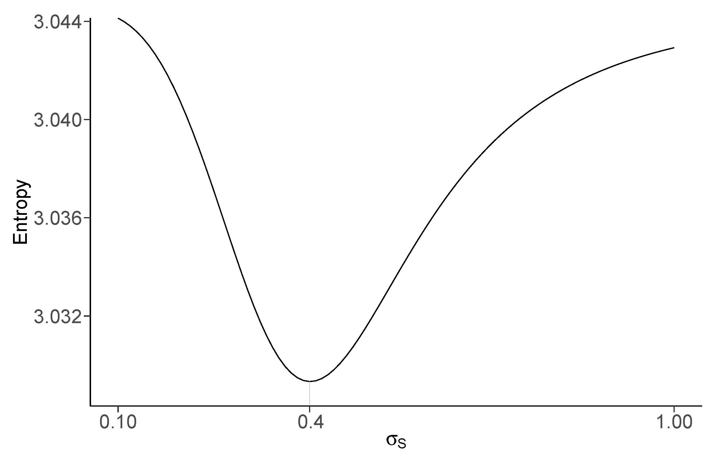
4.3. Selection of
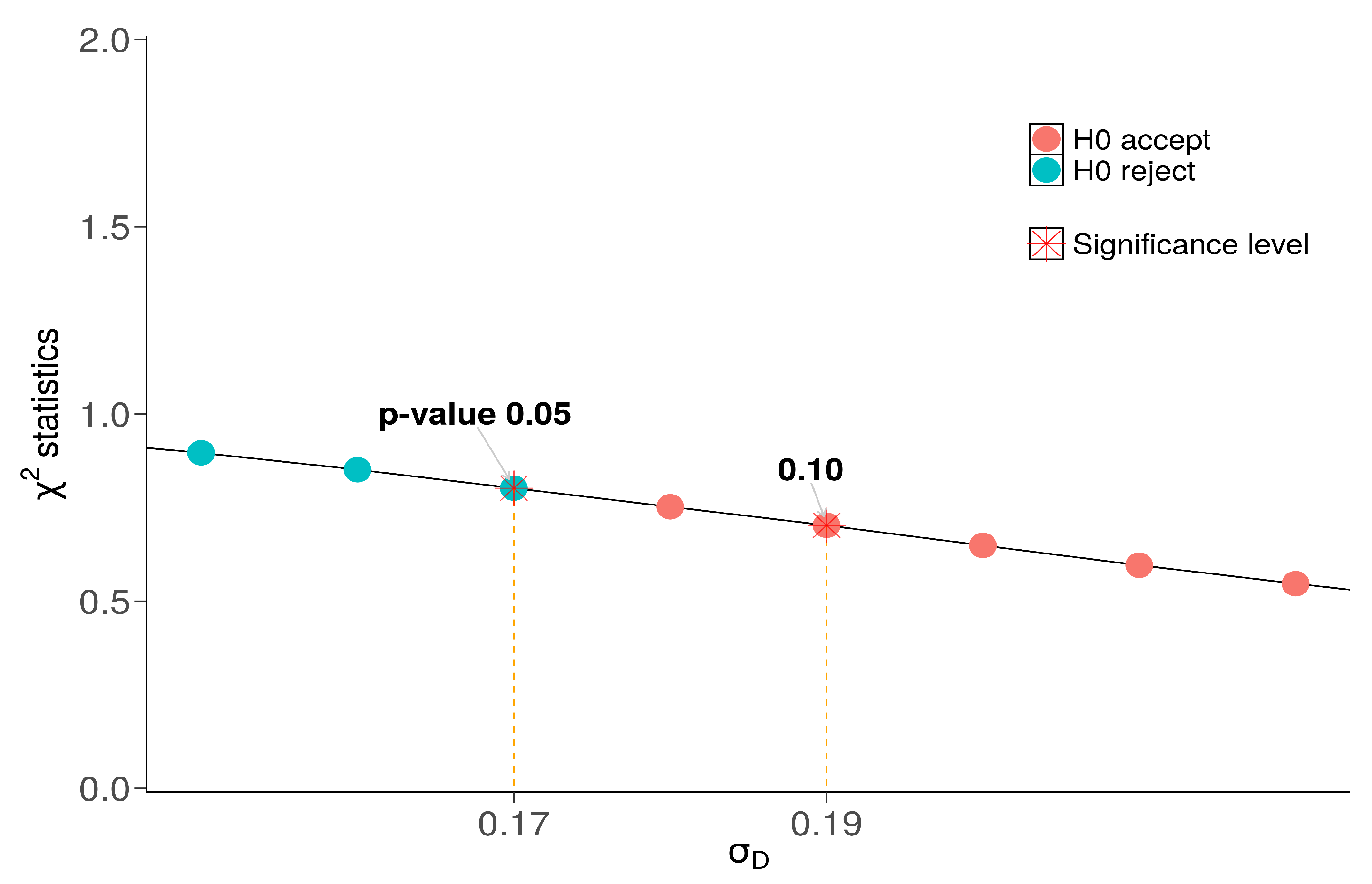
4.4. Selection of
- Step 1: Generate random weights from the Dirichlet distribution with all parameters equal to 1 (under ), for ;
- Step 2: Compute , and denote it ;
- Step 3: Iterate the above two steps K (=1000, for example) times;
- Step 4: Calculate ,
5. Results: Model Weights
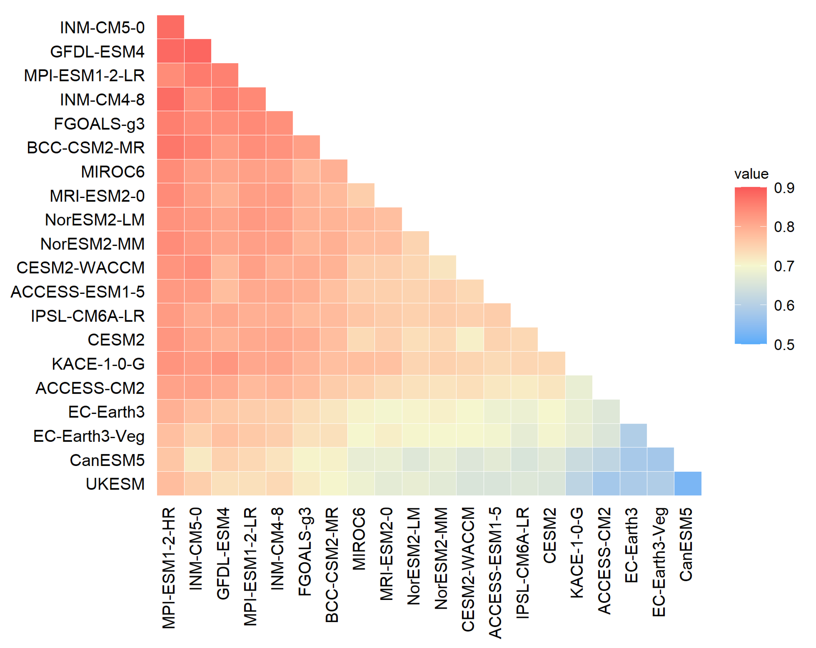
5.1. Model Similarity
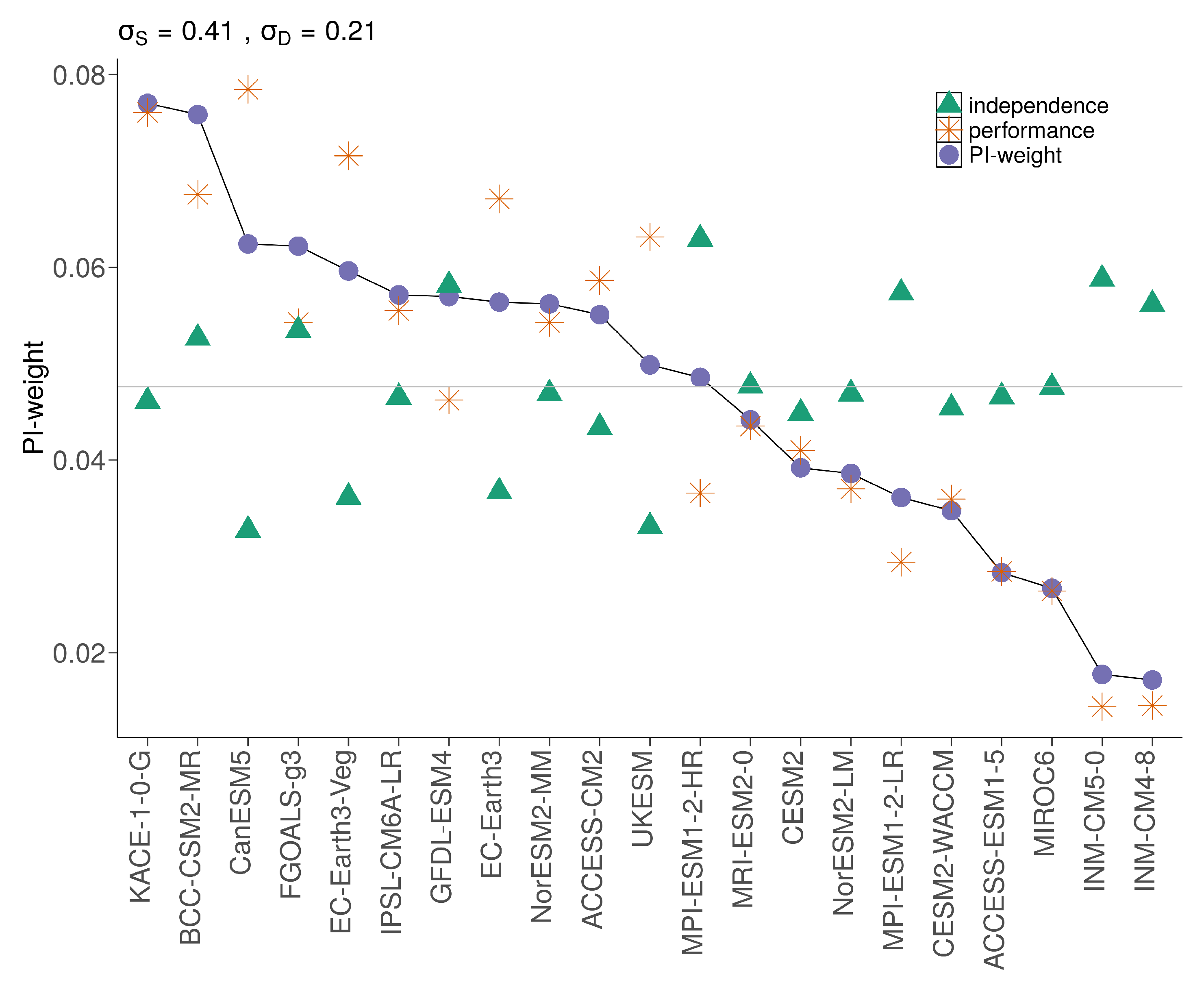
5.2. PI-Weights
6. Results: Future Projection of Extreme Precipitation
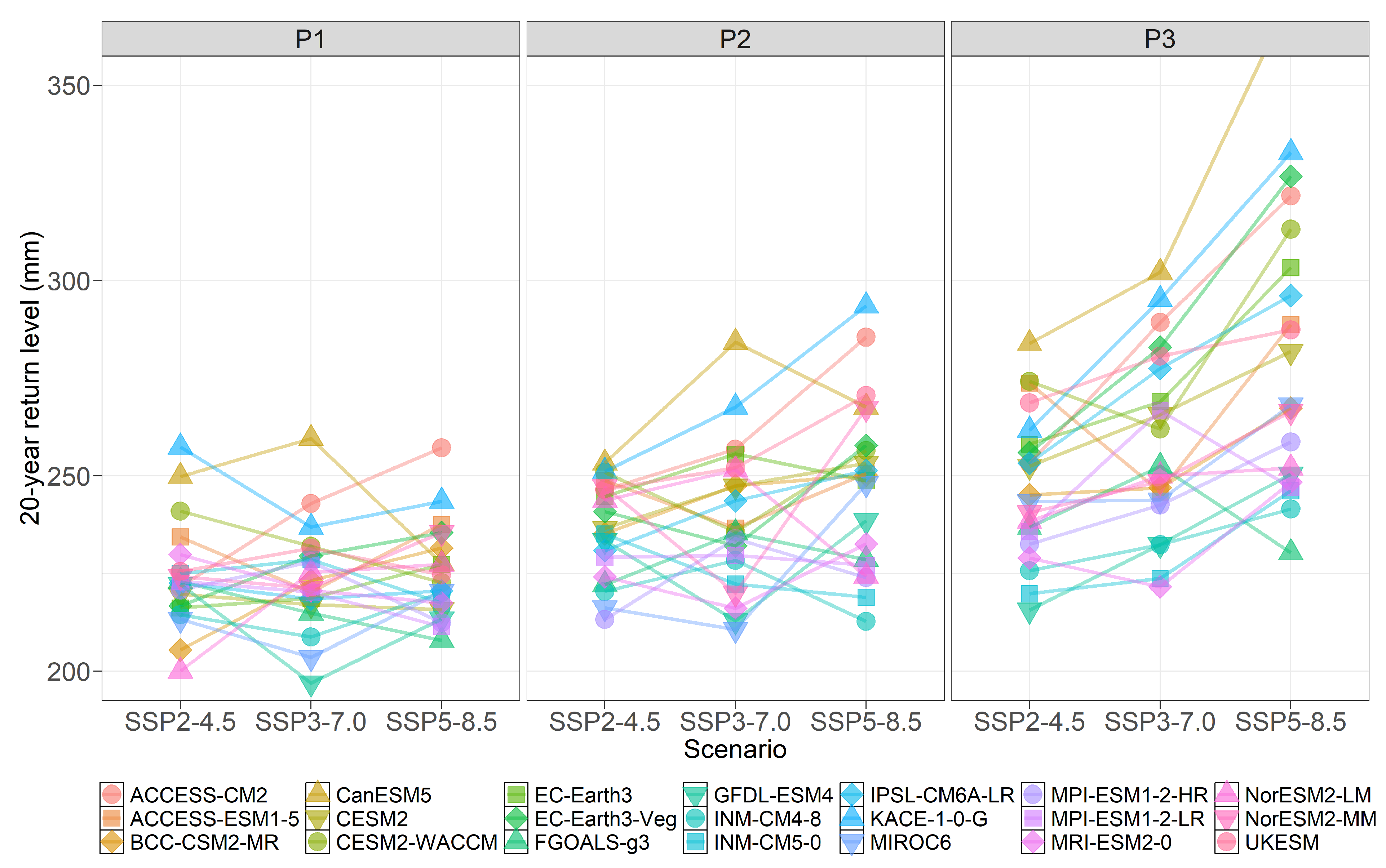
6.1. Return Levels
6.2. Changes in Return Levels
6.3. Change in Return Periods
6.4. Exceedance Probability and Waiting Time
6.5. Expected Number of Reoccurring Years
7. Results: Projection by Latitude and Quantifying Uncertainty
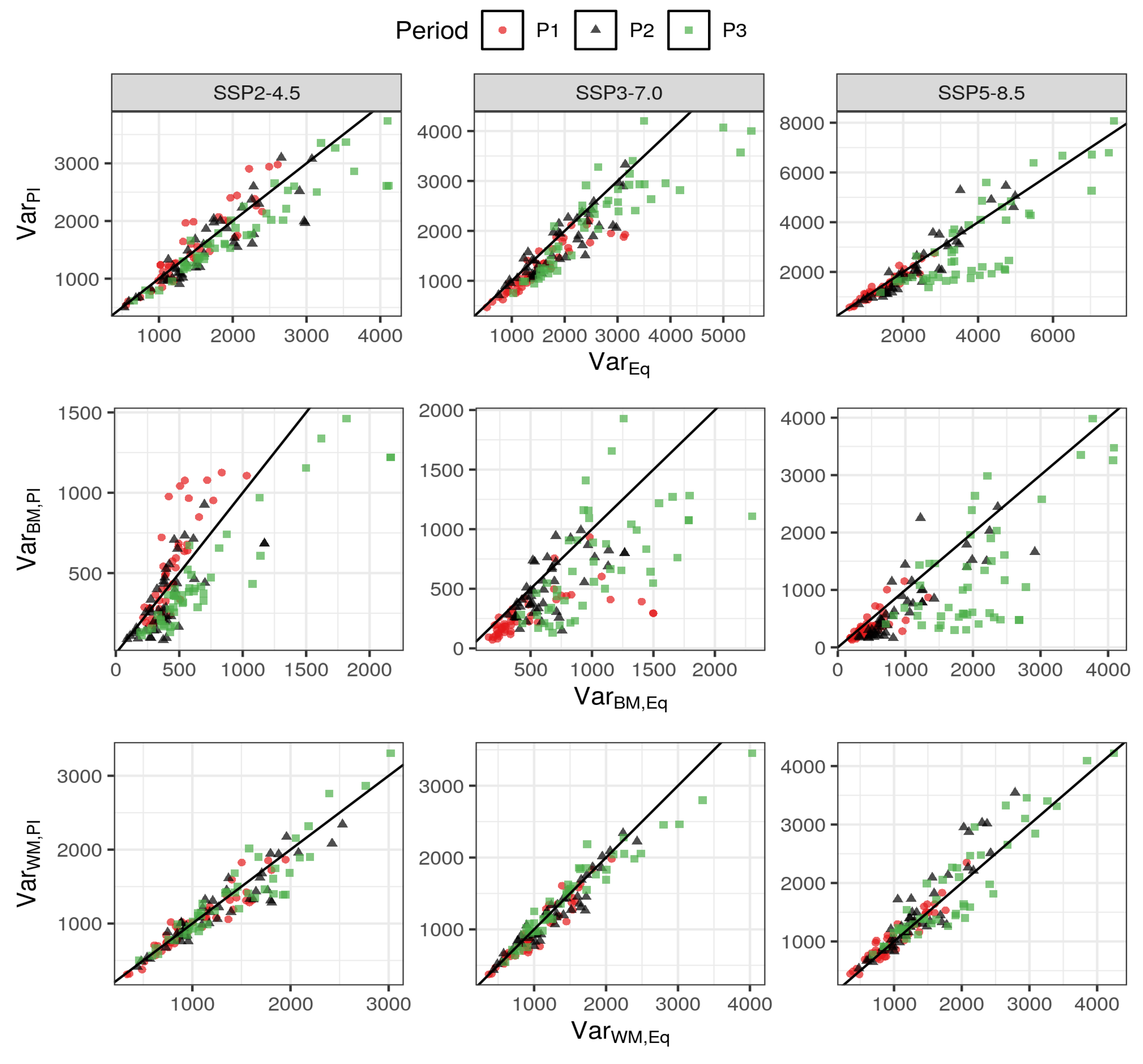
7.1. Variance Decomposition with Interaction
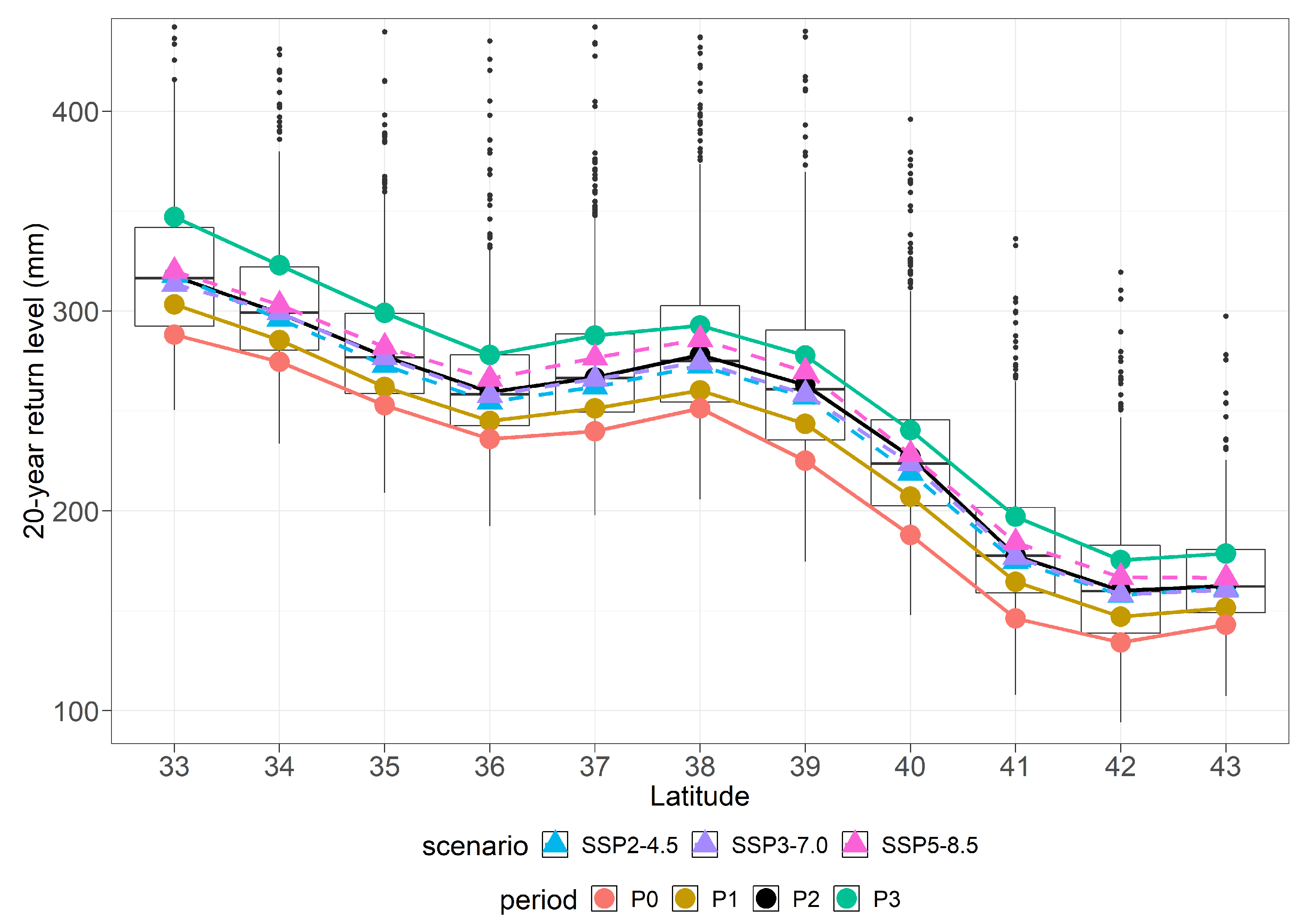
7.2. Return Levels by Latitude
8. Comparison of PI-Weighted Ensembles to the Simple Average
8.1. Error Index for the Historical Period
8.2. Prediction Variance for the Future
9. Discussion
10. Summary
Supplementary Materials
Author Contributions
Funding
Data Availability Statement
Acknowledgments
Conflicts of Interest
References
- IPCC. Managing the Risks of Extreme Events and Disasters to Advance Climate Change Adaptation. Special Report of the Intergovernmental Panel on Climate Change; Cambridge University Press: Cambridge, UK, 2012; Available online: http://ipcc-wg2.gov/SREX/report/ (accessed on 15 July 2020).
- Easterling, D.R.; Kunkel, K.E.; Arnold, J.R.; Knutson, T.; LeGrande, A.N.; Leung, L.R.; Vose, R.S.; Waliser, D.E.; Wehner, M.F. Precipitation Change in the United States. In Climate Science Special Report: Fourth National Climate Assessment; Wuebbles, D.J., Fahey, D.W., Hibbard, K.A., Dokken, D.J., Stewart, B.C., Maycock, T.K., Eds.; U.S. Global Change Research Program: Washington, DC, USA, 2017; Volume I, pp. 207–230. [Google Scholar] [CrossRef]
- Westra, S.; Alexander, L.V.; Zwiers, F.W. Global increasing trends in annual maximum daily precipitation. J. Clim. 2013, 26, 3904–3918. [Google Scholar] [CrossRef] [Green Version]
- Freychet, N.; Hsu, H.; Chou, C.; Wu, C. Asian summer monsoon in CMIP5 projections: A link between the change in extreme precipitation and monsoon dynamics. J. Clim. 2015. [Google Scholar] [CrossRef]
- Alexander, L.V. Global observed long-term changes in temperature and precipitation extremes: A review of progress and limitations in IPCC assessments and beyond. Weather. Clim. Extrem. 2016, 11, 4–16. [Google Scholar] [CrossRef] [Green Version]
- Park, C.; Min, S.K.; Lee, D.; Cha, D.H.; Suh, M.S.; Kang, H.K.; Hong, S.Y.; Lee, D.K.; Baek, H.J.; Boo, K.O.; et al. Evaluation of multiple regional climate models for summer climate extremes over East Asia. Clim. Dynam. 2016, 46, 2469–2486. [Google Scholar] [CrossRef]
- Dike, V.N.; Lin, Z.-H.; Ibe, C.C. Intensification of Summer Rainfall Extremes over Nigeria during Recent Decades. Atmosphere 2020, 11, 1084. [Google Scholar] [CrossRef]
- Lenderink, G.; van Meijgaard, E. Increase in hourly precipitation extremes beyond expectations from temperature changes. Nat. Geosci. 2008, 1, 511–514. [Google Scholar] [CrossRef]
- Berg, P.; Moseley, C.; Haerter, J.O. Strong increase in convective precipitation in response to higher temperatures. Nat. Geosci. 2013, 6, 181–185. [Google Scholar] [CrossRef]
- Scott, M. Prepare for More Downpours: Heavy Rain Has Increased across Most of the United States, and Is Likely to Increase Further. ClimateWatch Magazine; 2019. Available online: https://www.climate.gov/ (accessed on 25 July 2020).
- CISRO. Climate Change in Australia: Projections for Australia’s NRM Regions. Technical Report; 2015. Available online: https://www.climatechangeinaustralia.gov.au/media/ccia/2.1.6/cms_page_media/168/CCIA_2015_NRM_TechnicalReport_WEB.pdf (accessed on 15 May 2020).
- Mann, M.E.; Kump, L.R. Dire Predictions: Understanding Climate Change, 2nd ed.; DK Publishing: New York, NY, USA, 2015. [Google Scholar]
- Hov, Ø.; Cubasch, U.; Fischer, E.; Höppe, P.; Iversen, T.; Gunnar Kvamstø, N.; Kundzewicz, W.Z.; Rezacova, D.; Rios, D.; Duarte., S.F.; et al. Extreme Weather Events in Europe: Preparing for Climate Change Adaptation; Report produced by Norwegian Meteorological Institute in cooperation with EASAC; Norwegian Meteorological Institute: Oslo, Norway, 2013. [Google Scholar]
- Ho, C.-H.; Park, T.-W.; Jun, S.-Y.; Lee, M.-H.; Park, C.-E.; Kim, J.; Lee, S.-J.; Hong, Y.-D.; Song, C.-K.; Lee, J.-B. A projection of extreme climate events in the 21st century over East Asia using the community climate system model 3. Asia Pac. J. Atmos. Sci. 2011, 47, 329–344. [Google Scholar] [CrossRef]
- Kwon, S.H.; Kim, J.; Boo, K.O.; Shim, S.; Kim, Y.; Choi, J.; Byun, Y.H. Performance-based projection of the climate change effects on precipitation extremes in East Asia using two metrics. Intern. J. Climatol. 2019, 39, 2324–2335. [Google Scholar] [CrossRef]
- Mukherjee, S.; Aadhar, S.; Stone, D.; Mishra, V. Increase in extreme precipitation events under anthropogenic warming in India. Weather. Clim. Extrem. 2018, 20, 45–53. [Google Scholar] [CrossRef]
- Jung, H.S.; Choi, Y.E.; Lim, G.H. Recent trends in temperature and precipitation over South Korea. Int. J. Clim. 2002, 22, 1327–1337. [Google Scholar] [CrossRef]
- Choi, K.S.; Moon, J.Y.; Kim, D.W. The significant increase of summer rainfall occurring in Korea from 1998. Theor. Appl. Clim. 2010, 102, 275–286. [Google Scholar] [CrossRef]
- Park, J.-S.; Kang, H.-S.; Lee, Y.; Kim, M.-K. Changes in the extreme daily rainfall in South Korea. Intern. J. Clim. 2011, 31, 2290–2299. [Google Scholar] [CrossRef]
- Lee, Y.; Paek, J.; Park, J.S.; Boo, K.-O. Changes in temperature and rainfall extremes across East Asia in the CMIP5 ensemble. Theor. Appl. Clim. 2020, 141, 143–155. [Google Scholar] [CrossRef]
- Boo, K.O.; Kwon, W.T.; Baek, H.J. Change of extreme events of temperature and precipitation over Korea using regional projection of future climate change. Geophys. Res. Lett. 2006, 33, L01701. [Google Scholar] [CrossRef]
- Im, E.S.; Jung, I.W.; Bae, D.H. The temporal and spatial structures of recent and future trends in extreme indices over Korea from a regional climate projection. Int. J. Clim. 2011, 31, 72–86. [Google Scholar] [CrossRef]
- Seo, Y.A.; Lee, Y.; Park, J.-S.; Kim, M.-K.; Cho, C.; Baek, H.-J. Assessing changes in observed and future projected precipitation extremes in South Korea. Int. J. Clim. 2015, 35, 1069–1078. [Google Scholar] [CrossRef]
- Ahn, J.-B.; Jo, S.; Suh, M.-S.; Cha, D.-H.; Lee, D.-K.; Hong, S.Y.; Min, S.-K.; Park, S.-C.; Kang, H.-S.; Shim, K.-M. Changes of precipitation extremes over South Korea projected by the 5 RCMs under RCP scenarios. Asia Pac. J. Atmos. Sci. 2016, 52, 223–236. [Google Scholar] [CrossRef]
- Cha, D.-H.; Lee, D.-K.; Jin, C.-S.; Kim, G.; Choi, Y.; Suh, M.-S.; Ahn, J.-B.; Hong, S.-Y.; Min, S.-K.; Park, S.-C.; et al. Future changes in summer precipitation in regional climate simulations over the Korean Peninsula forced by multi-RCP scenarios of HadGEM2-AO. Asia. Pac. J. Atmos. Sci. 2016, 52, 139–149. [Google Scholar] [CrossRef]
- Kim, G.; Cha, D.-H.; Park, C.; Lee, G.; Jin, C.-S.; Lee, D.-K.; Suh, M.-S.; Ahn, J.-B.; Min, S.-K.; Hong, S.-Y.; et al. Future changes in extreme precipitation indices over Korea. Int. J. Clim. 2019, 38, 862–874. [Google Scholar] [CrossRef]
- Lee, Y.; Shin, Y.G.; Park, J.S.; Boo, K.O. Future projections and uncertainty assessment of precipitation extremes in the Korean peninsula from the CMIP5 ensemble. Atmos. Sci. Lett. 2020, e954. [Google Scholar] [CrossRef] [Green Version]
- O’Neill, B.C.; Kriegler, E.; Riahi, K.; Ebi, K.L.; Hallegatte, S.; Carter, T.R.; Mathur, R.; van Vuuren, D.P. A new scenario framework for climate change research: The concept of Shared Socioeconomic Pathways. Clim. Chang. 2014, 122, 387–400. [Google Scholar] [CrossRef] [Green Version]
- Tebaldi, C.; Hayhoe, K.; Arblaster, J.M.; Meehl, G.A. Going to the extremes: An intercomparison of model-simulated historical and future changes in extreme events. Clim. Chang. 2006, 79, 185–211. [Google Scholar] [CrossRef]
- Knutti, R. The end of model democracy? Clim. Chang. 2010, 102, 394–404. [Google Scholar] [CrossRef]
- Suh, M.S.; Oh, S.G.; Lee, D.K.; Cha, D.H.; Choi, S.-J.; Jin, C.-S.; Hong, S.-Y. Development of new ensemble methods based on the performance skills of regional climate models over South Korea. J. Clim. 2012, 25, 7067–7082. [Google Scholar] [CrossRef] [Green Version]
- Sanderson, B.M.; Knutti, R.; Caldwell, P. A representative democracy to reduce interderpendency in a multimodel ensemble. J. Clim. 2015, 28, 5171–5194. [Google Scholar] [CrossRef] [Green Version]
- Massoud, E.C.; Espinoza, V.; Guan, B.; Waliser, D.E. Global Climate Model Ensemble Approaches for Future Projections of Atmospheric Rivers. Earth’s Future 2019, 7, 1136–1151. [Google Scholar] [CrossRef] [Green Version]
- Eyring, V.; Cox, P.M.; Flato, G.M.; Gleckler, P.J.; Abramowitz, G.; Caldwell, P.; William, D.C.; Bettina, K.G.; Alex, D.H.; Forrest, M.H.; et al. Taking climate model evaluation to the next level. Nat. Clim. Chang. 2019, 9, 102–110. [Google Scholar] [CrossRef] [Green Version]
- Xu, D.; Ivanov, V.; Kim, J.; Fatichi, S. On the use of observations in assessment of multi-model climate ensemble. Stoch. Environ. Res. Risk Assess. 2019, 33, 1923–1937. [Google Scholar] [CrossRef]
- Brunner, L.; Lorenz, R.; Zumwald, M.; Knutti, R. Quantifying uncertainty in European climate projections using combined performance-independence weighting. Environ. Res. Lett. 2019, 14, 124010. [Google Scholar] [CrossRef]
- Georgi, F.; Mearns, L.O. Calculation of average, uncertainty range and reliability of regional climate changes from AOGCM simulations via the ‘Reliability Ensemble Averaging (REA)’ method. J. Clim. 2002, 15, 1141–1158. [Google Scholar] [CrossRef]
- Abramowitz, G.; Gupta, H. Toward a model space and model independence metric. Geophys. Res. Lett. 2008, 35, L05705. [Google Scholar] [CrossRef] [Green Version]
- Knutti, R.; Sedlacek, J.; Sanderson. B.M.; Lorenz, R.; Fischer, E.M.; Eyring, V. A climate model projection weighting scheme accounting for performance and independence. Geophys. Res. Lett. 2017, 44, 1909–1918. [Google Scholar]
- Lorenz, R.; Herger, N.; Sedlacek, J.; Eyring, V.; Fischer, E.M.; Knutti, R. Prospects and caveats of weighting climate models for summer maximum temperature projections over North America. J. Geophys. Res. Atmos. 2018, 123, 4509–4526. [Google Scholar] [CrossRef]
- Shin, Y.; Lee, Y.; Park, J.S. A Weighting Scheme in A Multi-Model Ensemble for Bias-Corrected Climate Simulation. Atmosphere 2020, 11, 775. [Google Scholar] [CrossRef]
- Karl, T.R.; Nicholls, N.; Ghazi, A. CLIVAR/GCOS/WMO workshop on indices and indicators for climate extremes: Workshop summary. Clim. Chang. 1999, 42, 3–7. [Google Scholar]
- Peterson, T.C.; Foll, C.; Gruza, G.; Hogg, W.; Mokssit, A.; Plummer, N. Report on the Activities of the Working Group on Climate Change Detection and Related Rapporteurs 1998–2001; Rep. WCDMP-47, WMO-TD 1071; WMO: Geneve, Switzerland, 2001; 143p, Available online: https://www.clivar.org/sites/default/files/documents/048_wgccd.pdf (accessed on 15 November 2020).
- Koch, S.E.; DesJardins, M.; Kocin, P.J. An interactive Barnes objective map analysis scheme for use with satellite and conventional data. J. Clim. Appl. Meteorol. 1983, 22, 1487–1503. [Google Scholar] [CrossRef]
- Zhou, B.; Wen, Q.H.; Xu, Y.; Song, L.; Zhang, X. Projected changes in temperature and precipitation extremes in China by the CMIP5 multimodel ensembles. J. Clim. 2014, 27, 6591–6611. [Google Scholar] [CrossRef]
- Li, D.; Zhou, T.; Zou, L.; Zhang, W.; Zhang, L. Extreme high-temperature events over East Asia in 1.5 °C and 2 °C warmer futures: Analysis of NCAR CESM low-warming experiments. Geophys. Res. Lett. 2018, 45, 1541–1550. [Google Scholar] [CrossRef] [Green Version]
- Kitoh, A.; Endo, H.; Kumar, K.K.; Iracema Fonseca de Albuquerque Cavalcanti. Monsoon in a changing world: A reginal perspective in a global context. J. Geophys. Res. Atmos. 2013, 118, 3053–3065. [Google Scholar] [CrossRef] [Green Version]
- The Regional Climate Group at the University of Gothenburg. Originated from Data Center of China Meteorological Administrator. Available online: http://rcg.gvc.gu.se/ (accessed on 15 July 2020).
- Japan Meteorological Agency. Available online: http://www.jma.go.jp/jma/index.html (accessed on 15 July 2020).
- Korean Meteorological Administration. Available online: https://data.kma.go.kr/cmmn/main.do (accessed on 1 March 2020).
- Yatagai, A.; Kamiguchi, K.; Arakawa, O.; Hamada, A.; Yasutomi, N.; Kitoh, A. APHRODITE: Constructing a long-term daily griddied precipitation dataset for Asia based on a dense network of rain gauges. Bull. Am. Meteorol. Soc. 2012, 93, 1401–1415. [Google Scholar] [CrossRef]
- Maraun, D.; Widmann, M. Statistical Downscaling and Bias Correction for Climate Research; Cambridge University Press: Cambridge, UK, 2018. [Google Scholar]
- Coles, S. An Introduction to Statistical Modelling of Extreme Values; Springer: New York, NY, USA, 2001; p. 224. [Google Scholar]
- Wilks, D. Statistical Methods in the Atmospheric Sciences, 3rd ed.; Academic Press: New York, NY, USA, 2011. [Google Scholar]
- Hosking, J.R.M.; Wallis, J.R. Regional Frequency Analysis: An Approach Based on L-Moments; Cambridge University Press: Cambridge, UK, 1997; 244p. [Google Scholar]
- Hosking, J.R.M. L-Moments. R Package, Version 2.8. 2019. Available online: https://CRAN.R-project.org/package=lmom (accessed on 5 March 2020).
- Christensen, J.H.; Boberg, F.; Christensen, O.B.; Lucas-Picher, P. On the need for bias correction of regional climate change projections of temperature and precipitation. Geophys. Res. Lett. 2008, 35, L20709. [Google Scholar] [CrossRef]
- Vrac, M.; Friederichs, P. Multivariate-intervariable, spatial, and temporal-bias correction. J. Clim. 2015, 28, 218–237. [Google Scholar] [CrossRef]
- Cannon, A.J. Multivariate quantile mapping bias correction: An N-dimensional probability density function transform for climate model simulations of multiple variables. Clim. Dyn. 2018, 50, 31–49. [Google Scholar] [CrossRef] [Green Version]
- Sanderson, B.M.; Knutti, R.; Caldwell, P. Addressing interdependency in a multimodel ensemble by interpolation of model properties. J. Clim. 2015, 28, 5150–5170. [Google Scholar] [CrossRef]
- Brunner, L.; Pendergrass, A.G.; Lehner, F.; Merrifield, A.L.; Lorenz, R.; Knutti, R. Reduced global warming from CMIP6 projections when weighting models by performance and independence. Earth Syst. Dyn. Discuss. 2020, 11, 995–1012. [Google Scholar] [CrossRef]
- Ross, S. A First Course in Probability, 8th ed.; Pearson Prentice Hall: Upper Saddle River, NJ, USA, 2010. [Google Scholar]
- Everitt, B.S.; Skrondal, A. The Cambridge Dictionary of Statistics; Cambridge University Press: Cambridge, UK, 2010. [Google Scholar]
- Martin, A.D.; Quinn, K.M.; Park, J.H. MCMCpack: Markov Chain Monte Carlo in R. J. Stat. Softw. 2011, 42, 1–21. [Google Scholar] [CrossRef] [Green Version]
- Kharin, V.V.; Zwiers, F.W.; Zhang, X.; Wehner, M. Changes in temperature and precipitation extremes in the CMIP5 ensemble. Clim. Chang. 2013, 119, 345–357. [Google Scholar] [CrossRef]
- Serinaldi, F. Dismissing return periods! Stoch. Environ. Res. Risk Assess. 2015, 29, 1179–1189. [Google Scholar] [CrossRef] [Green Version]
- Paciorek, C.J.; Stone, D.A.; Wehner, M.F. Quantifying statistical uncertainty in the attribution of human influence on severe weather. Weather. Clim. Extrem. 2018, 20, 69–80. [Google Scholar] [CrossRef]
- Hawkins, E.; Sutton, R.T. The potential to narrow uncertainty in regional climate predictions. Bull. Am. Meteorol. Soc. 2009, 90, 1095–1107. [Google Scholar] [CrossRef] [Green Version]
- Yip, S.; Ferro, C.A.T.; Stephenson, D.B. A simple, coherent framework for partitioning uncertainty in climate predictions. J. Clim. 2011, 24, 4634–4643. [Google Scholar] [CrossRef]
- Baker, N.C.; Taylor, P.C. A framework for evaluating climate model performance metrics. J. Clim. 2016, 29, 1773–1782. [Google Scholar] [CrossRef]
- Draper, D. Assessment and propagation of model uncertainty. J. R. Stat. Soc. Ser. B 1995, 57, 45–97. [Google Scholar] [CrossRef]
- Zhu, J.; Forsee, W.; Schumer, R.; Gautam, M. Future projections and uncertainty assessment of extreme rainfall intensity in the United States from an ensemble of climate models. Clim. Chang. 2013, 118, 469–485. [Google Scholar] [CrossRef]
- Ruckstuhl, C.; Philipona, R.; Morl, J.; Ohmura, A. Observed relationship between surface specific humidity, integrated water vapor, and longwave downward radiation at different altitudes. J. Geophys. Res. Atmos. 2007, 112, 1–7. [Google Scholar] [CrossRef]
- Kendon, E.J.; Rowell, D.P.; Jones, R.G.; Buonomo, E. Robustness of future changes in local precipitation extremes. J. Clim. 2008, 21, 4280–4297. [Google Scholar] [CrossRef]
- Sillmann, J.; Kharin, V.V.; Zhang, X.; Zwiers, F.W.; Bronaugh, D. Climate extremes indices in the CMIP5 multimodel ensemble: Part 1. Model evaluation in the present climate. J. Geophy. Res. Atmos. 2013, 118, 1–18. [Google Scholar] [CrossRef]


| Variable Acronym | Description |
|---|---|
| AMP1 | Annual Maximum Daily Precipitation |
| AMP5 | Annual Maximum Five-Day Precipitation |
| ATP | Annual Total Precipitation |
| AMCWD | Annual Maximum Consecutive Wet Days |
| AMCDD | Annual Maximum Consecutive Dry Days |
| SSP2-4.5 | SSP3-7.0 | SSP5-8.5 | ||||||||
|---|---|---|---|---|---|---|---|---|---|---|
| AMP1 | OBS | P1 | P2 | P3 | P1 | P2 | P3 | P1 | P2 | P3 |
| 100 mm | 1.8 | 1.4 | 1.3 | 1.3 | 1.4 | 1.3 | 1.2 | 1.4 | 1.3 | 1.2 |
| 150 mm | 4.4 | 4.4 | 3.9 | 3.7 | 4.0 | 3.2 | 2.5 | 3.6 | 3.0 | 2.5 |
| 200 mm | 11.1 | 14.5 | 11.1 | 10.6 | 13.2 | 10.2 | 7.1 | 13.0 | 8.0 | 5.9 |
| 250 mm | 30.7 | 41.7 | 31.7 | 27.1 | 42.9 | 28.7 | 16.9 | 34.4 | 24.9 | 15.0 |
| 300 mm | 78 | 93 | 76 | 55 | 104 | 59 | 42 | 76 | 50 | 29 |
| 400 mm | 485 | 400 | 297 | 202 | 469 | 254 | 201 | 227 | 166 | 107 |
| 500 mm | 1970 | 1167 | 814 | 577 | 1148 | 649 | 563 | 538 | 493 | 307 |
| 20-Year Return Level (AMP1) | 20-Year Return Level (AMP5) | |||||||
|---|---|---|---|---|---|---|---|---|
| Latitude | OBS | OBS | ||||||
| 33 | 288 | 303 | 319 | 345 | 443 | 440 | 471 | 519 |
| 34 | 275 | 288 | 303 | 329 | 416 | 416 | 446 | 487 |
| 35 | 253 | 264 | 280 | 305 | 384 | 386 | 412 | 445 |
| 36 | 235 | 246 | 261 | 282 | 360 | 368 | 389 | 414 |
| 37 | 243 | 252 | 270 | 296 | 396 | 409 | 429 | 461 |
| 38 | 249 | 262 | 281 | 302 | 402 | 419 | 438 | 466 |
| 39 | 227 | 245 | 267 | 287 | 377 | 398 | 417 | 442 |
| 40 | 186 | 209 | 227 | 247 | 299 | 319 | 337 | 357 |
| 41 | 147 | 166 | 181 | 201 | 236 | 249 | 266 | 285 |
| 42 | 136 | 149 | 164 | 181 | 207 | 213 | 235 | 250 |
| 43 | 143 | 151 | 167 | 184 | 223 | 227 | 254 | 271 |
| ssp | p | BSS(%) | DV | RI(%) | ||||
|---|---|---|---|---|---|---|---|---|
| P1 | −2.2 | −12.3 | 2.0 | −50 | −77 | 27 | −3.3 | |
| SSP2-4.5 | P2 | 7.7 | 19.7 | 3.2 | 129 | 82 | 47 | 8.5 |
| P3 | 13.4 | 39.0 | 2.7 | 309 | 267 | 42 | 17.1 | |
| P1 | 17.9 | 42.9 | 5.4 | 300 | 238 | 62 | 24.0 | |
| SSP3-7.0 | P2 | 11.0 | 22.5 | 4.7 | 228 | 153 | 75.0 | 13.7 |
| P3 | 16.7 | 36.2 | 1.4 | 426 | 378 | 48 | 19.5 | |
| P1 | 6.4 | 24.7 | −4.5 | 113 | 138 | −25 | 8.0 | |
| SSP5-8.5 | P2 | 10.4 | 33.9 | −6.9 | 178 | 291 | −113 | 8.0 |
| P3 | 22.5 | 42.2 | −1.1 | 826 | 834 | −8 | 26.0 |
Publisher’s Note: MDPI stays neutral with regard to jurisdictional claims in published maps and institutional affiliations. |
© 2021 by the authors. Licensee MDPI, Basel, Switzerland. This article is an open access article distributed under the terms and conditions of the Creative Commons Attribution (CC BY) license (http://creativecommons.org/licenses/by/4.0/).
Share and Cite
Shin, Y.; Shin, Y.; Hong, J.; Kim, M.-K.; Byun, Y.-H.; Boo, K.-O.; Chung, I.-U.; Park, D.-S.R.; Park, J.-S. Future Projections and Uncertainty Assessment of Precipitation Extremes in the Korean Peninsula from the CMIP6 Ensemble with a Statistical Framework. Atmosphere 2021, 12, 97. https://0-doi-org.brum.beds.ac.uk/10.3390/atmos12010097
Shin Y, Shin Y, Hong J, Kim M-K, Byun Y-H, Boo K-O, Chung I-U, Park D-SR, Park J-S. Future Projections and Uncertainty Assessment of Precipitation Extremes in the Korean Peninsula from the CMIP6 Ensemble with a Statistical Framework. Atmosphere. 2021; 12(1):97. https://0-doi-org.brum.beds.ac.uk/10.3390/atmos12010097
Chicago/Turabian StyleShin, Yonggwan, Yire Shin, Juyoung Hong, Maeng-Ki Kim, Young-Hwa Byun, Kyung-On Boo, Il-Ung Chung, Doo-Sun R. Park, and Jeong-Soo Park. 2021. "Future Projections and Uncertainty Assessment of Precipitation Extremes in the Korean Peninsula from the CMIP6 Ensemble with a Statistical Framework" Atmosphere 12, no. 1: 97. https://0-doi-org.brum.beds.ac.uk/10.3390/atmos12010097